Search for $C=+$ charmonium and bottomonium states in $e^{+}e^{-}\to\gamma+~X$ at B factories

In recent years there have been a number of exciting discoveries of new hidden charm states, i.e. the so called XYZ mesons, by Belle, BaBar, CLEO, CDF, and D0 collaborations (for recent experimental and theoretical reviews and related references see Ref.[1]). Among the XYZ states, the charge parity C=+ states such as X(3872), X(3940), Y(3940), Z(3930), and X(4160) are particularly interesting and the interpretations for their nature are still very inconclusive (except for the Z(3930), which is assigned as the $\chi_{c2}(2P)$ meson). The experimental results for these C=+ states have induced renewed theoretical interest in understanding the mass spectrum, decay and production mechanisms of charmonium or charmoniumlike states (see, e.g., Refs.[1, 2, 3, 4, 5]). Among others, the double charmonium production in $e^{+}e^{-}$ annihilation at B-factories[6, 7] turned out to be a good way to find the C=+ charmonium or charmoniumlike states, recoiling against the easily reconstructed $1^{--}$ charmonium $J/\psi$ and $\psi(2S)$. In addition to the $\eta_{c},\eta_{c}(2S)$ and $\chi_{c0}$, the $X(3940)$ (decaying into $D\bar{D^{*}}$) and $X(4160)$ (decaying into $D^{*}\bar{D^{*}}$) have also been observed in double charmonium production. Since the quantum number of the photon is the same as $J/\psi$, it will be interesting to see whether the C=+ charmonium or charmoniumlike states can be found in the process $e^{+}e^{-}\to\gamma^{*}\to\gamma+X$, where $X$ is a C=+ state recoiling against the photon. The production rates of such processes have been calculated at tree level in QED[8].

It has been known for some time that the one-loop QCD radiative corrections are very important in double charmonium production in $e^{+}e^{-}$ annihilation. The observed double charmonium production cross section[6, 7] for $e^{+}e^{-}\to J/\psi\eta_{c}$ is larger than the leading-order (LO) calculations in NRQCD[9] by an order of magnitude[10], and later it was found that these discrepancies could be largely resolved by the next-to-leading-order (NLO) QCD corrections[11, 12] combined with relativistic corrections[13, 14]. Therefore, it is necessary to examine whether the one-loop QCD (i.e., $O(\alpha_{s})$) corrections are also important for the processes $e^{+}e^{-}\to\gamma^{*}\to\gamma+X$. In fact, the one-loop QCD radiative correction to $e^{+}e^{-}\to\gamma^{*}\to\gamma+\eta_{c}$ has been investigated elsewhere[15, 16].

Another interesting point is about $1^{++}$ charmonium. At $B$ factories the observed production cross sections in $e^{+}e^{-}$ annihilation to $J/\psi\eta_{c}$, $\psi(2S)\eta_{c}$, $J/\psi\eta_{c}(2S)$, $J/\psi\chi_{c0}$, and $\psi(2S)\chi_{c0}$ are large, but no signals for $J/\psi\chi_{c1,2}$ have been seen. This is in line with the calculations in NRQCD[10], in which the predicted production rates of $J/\psi\chi_{c1,2}$ are relatively suppressed. We wonder whether the cross section of $1^{++}$ charmonium (including $\chi_{c1}$ and its radial excitations) associated with a photon could be large in $e^{+}e^{-}\to\gamma^{*}\to\gamma+X$. If this is the case, we might have a chance to search for the $\chi_{c1}$ as well as the X(3872) in $e^{+}e^{-}\to\gamma^{*}\to\gamma+X$, since the X(3872) could be a $\chi_{c1}(2P)$ dominated state but mixed with some $D^{0}\bar{D^{*0}}$ component, in one of the possible interpretations. This is also useful to the search for the Y(3940), which has been seen in the decay $B\to Y(3940)K$ followed by $Y(3940)\to J/\psi\omega$, and is also a possible candidate for the $\chi_{c1}(2P)$ (or $\chi_{c0}(2P)$). Of course, these states could have some more exotic nature, being molecules, tetraquarks, or charmonium hybrids.

In this paper, we compute the QED (at tree level) and one-loop QCD ($O(\alpha_{s})$) corrections to the processes $e^{+}e^{-}\to\gamma^{*}\to\gamma+X$, where X are $\chi_{cJ},\eta_{c},{}^{1}D_{2}$ and their radially excited states, all with charge-parity $C=+1$. We find the cross sections for $\eta_{c}$, its radial excited states and $\chi_{c1}$, $\chi_{c1}(2P)$ are relatively large. Despite of the large background from initial state radiation (ISR), we still expect they could be seen in the $\gamma$ recoil spectrum with higher statistics in the future. The remainder of the paper is organized as follows. In Sec.2 we outline the QED calculation and some basic techniques for numerically computing the one-loop QCD correction. The QED and one-loop QCD corrections to cross sections for $e^{+}e^{-}\to\gamma+X$ at B factories are given in Sec. 4, and we also analyze and discuss our results. In the Appendix, we show some basic integration expressions.

The Feynman diagram for the exclusive process $e^{+}e^{-}\longrightarrow\gamma+X$ at order $\alpha^{3}\alpha_{s}^{0}$ is shown in Fig.1, where X is a heavy quarkonium with charge-parity $C=+1$, and there is another quark line-flipped one. In the nonrelativistic limit, the factorization formula for heavy quarkonium production in the NRQCD framework is equivalent to that in the color-singlet model. And in our case, the amplitude $\mathcal{M}$ for $e^{+}e^{-}\to\gamma+X$ can be expressed as

where $P$ is the momentum of $X$ state, $2q$ is relative momentum between $Q$ and $\overline{Q}$ in the rest frame of X state, and $\langle LL_{z};SS_{z}|JJ_{z}\rangle$, $\langle s_{1};s_{2}|SS_{z}\rangle$ and $\langle i,j|1\rangle=\delta_{i,j}/\sqrt{N_{c}}$ are the spin-SU(2), angular momentum C-G coefficients and color-SU(3) C-G coefficients for $Q\bar{Q}$ pairs projecting onto appropriate bound states respectively. And $\mathcal{A}$ is the standard Feynman amplitude denoting $e^{+}e^{-}\to\gamma+Q_{s_{1}}^{i}(\frac{P}{2}+q)+\overline{Q}_{s_{2}}^{j}(\frac{P}{2}-q)$.

The Feynman amplitude part can be evaluated by introducing the spin projection operator[17, 18]:

Expanding the operator in terms of the relative momentum $q$, we get the leading-order nonvanishing terms for the $S$-, $P$- and $D$-wave case respectively. The results of the spin-triplet and spin-singlet projection operators and their derivatives with respective to the relative momentum $q_{\alpha}$ are given below[19]:

After integrating $q^{0}$, we get the amplitudes for $S$, $P$ and $D$-wave heavy quarkonium production respectively:

where $O$ is the $\gamma$ matrix relevant to the Feynman amplitude $\mathcal{A}$, and $O^{\alpha}$ and $O^{\alpha\beta}$ are the first and second derivatives of $O$ with respect to $q_{\alpha}$ respectively.

The integrals of the wave function in momentum space are related to the radial wave function $R_{S}(0)$, $R_{P}^{\prime}(0)$ and $R_{D}^{\prime\prime}(0)$ in coordinator space at the origin for the $S-$, $P-$ and $D-$ wave cases respectively:

where $\epsilon^{\alpha}(L_{z})$ is the polarization vector of $L=1$ ($P$-wave) system and $\varepsilon_{\alpha\beta}^{m}(L_{z})$ is the polarization tensor of $L=2$ ($D$-wave) system.

For spin-triplet $P$-wave states, the projection of the $L-S$ coupling of the spin vector $\epsilon^{\ast}(S_{z})$ and orbital vector $\epsilon^{\ast}(L_{z})$ onto total angular momentum $J$ for $J=0,1,2$ are

where $\Pi_{\alpha\beta}=(-g_{\alpha\beta}+\frac{P_{\alpha}P_{\beta}}{4m_{Q}^{2}})$. For the total angular momentum $J=1$ and $J=2$ states, the sums over all possible polarizations are given by

With the help of the formula introduced above, we get the final QED analytic expressions for the exclusive process $e^{+}e^{-}\longrightarrow\gamma+X$:

where $r=M_{x}^{2}/s$, $\cos(\theta)$ is the angle between $J/\psi$ and the initial beam axis. For the $c\bar{c}$ system we set $M_{X}=2m_{c}$. If we replace $\frac{3}{4\pi}|R^{\prime}_{p}(0)|^{2}$ by $\frac{1}{N_{c}^{2}-1}\frac{\langle O_{8}({}^{3}P_{J})\rangle}{2J+1}$, we find our QED results of ${}^{3}P_{J}$ are consistent with those in Ref.[20]. For $b\bar{b}$ states, the result can be obtained by changing $e_{c}$ to $e_{b}$, $m_{c}$ to $m_{b}$ and the values of the wave-functions for charmonium states to those for bottomonium states.

Now we proceed to calculate the one-loop QCD corrections. The numerical calculation of one-loop QCD corrections is performed with the help of Feyncalc and Looptools. At the one-loop level of QCD, there are eight Feynman diagrams. We show four of them in Fig.2, and the other four can be obtained by reversing the direction of the charm quark line.

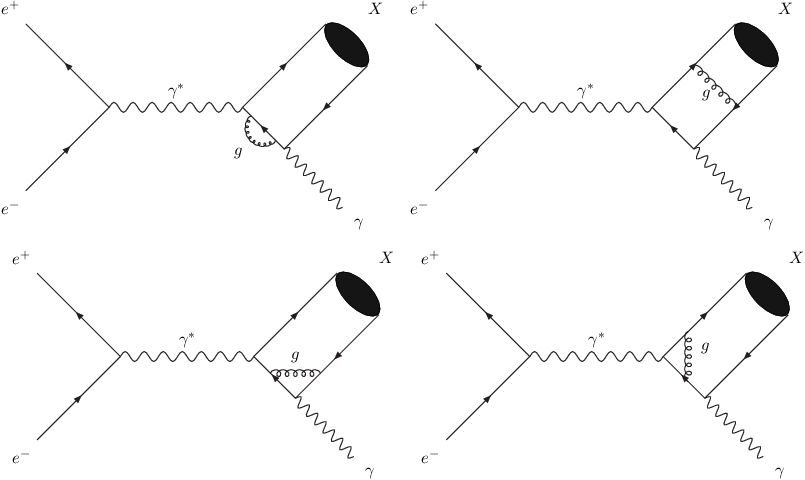
At order $\alpha^{3}\alpha_{s}$, the cross section for $e^{+}e^{-}\longrightarrow\gamma+X$ is

where $\mathcal{M}_{QCD}$ means the one-loop QCD amplitude. The on-shell scheme is adopted and then the self-energy renormalization constant $Z_{1}$ and vertex renormalization constant $Z_{2}$ are chosen to be

where we omit the coefficient before the self-energy renormalization constant and part of the infrared divergence term in $\delta Z_{2}^{OS}$.

In the S-wave case, we encounter the $C_{0}$ function in box diagram, with the analytic formula[11]:

The infrared divergence $\epsilon$ is canceled by the IR divergence term in self-energy and vertex renormalization constants, and the Coulomb singularity term with $\frac{1}{v}$ pole can be absorbed into the wave-function by

In the P-wave case, we have to deal with loop-integrals typically as the following expression in the box diagram when taking derivative of the relative momentum $q_{\alpha}$ on the denominator of the propagators

where $2p_{1}$ is the momentum of the heavy quarkonium and $p_{2}$ is the momentum of the photon. The contribution which is proportional to the $p_{1}^{\alpha}$ term will be omitted when contracted with polarization vector. Using the identity $A(l)=(A(l)-A(0))+A(0)$, we can separate the IR divergence into the second term which will be canceled by other diagrams. Three types of integrations will appear here, which are given in the Appendix.

In treating the first term, with the help of the formula $l\cdot p_{1}=(l^{2}-((l-p_{1})^{2}-m_{Q}^{2}))/2$ and Dirac decomposition: $l^{\mu}l^{\nu}=g^{\mu\nu}I_{1}+p_{1}^{\mu}p_{1}^{\nu}I_{2}+(p_{1}^{\mu}p_{2}^{\nu}+p_{1}^{\nu}p_{2}^{\mu})I_{3}+p_{2}^{\mu}p_{2}^{\nu}I_{4}$, we are able to evaluate most of terms by using LoopTools. Note that to get the correct result of the integration $\int d^{4}l\frac{1}{((l-p_{1})^{2}-m^{2})^{2}((l+p_{1})^{2}-m^{2})}$ the small number $i\varepsilon$ in the propagators should be kept. And we have checked the independence of the final result on $\varepsilon$.

The analytical method is also performed to calculate the one-loop QCD corrections as a cross-check for the numerical results. We find the results of the two different methods are in agreement.

We choose $\sqrt{s}=10.6$ GeV, $m_{c}$=1.5 GeV, $m_{b}$=4.7 GeV, $\alpha_{s}(2m_{c})$=0.26, $\alpha_{s}(2m_{b})$=0.18 as inputs. As for the charmonium wave-functions at the origin, we choose the results from potential model calculations (see the results of the $B-T$-type potential in Ref.[21]), which are listed in Table I. The results of cross sections for $e^{+}e^{-}\to\gamma^{*}\to\gamma+X$ are listed in Table II, where $\sigma_{QED}$ means the QED result and $\sigma_{QCD}$ means the corresponding one-loop QCD correction. However, if we extract the wave-functions at the origin from the observed charmonium decay (e.g., $J/\psi\to e^{+}e^{-}$ or $\eta_{c}\to 2\gamma$) widths using theoretical expressions with (without) NLO QCD corrections[18], then the obtained QED cross sections for $e^{+}e^{-}\to\gamma^{*}\to\gamma+X$ will be larger (smaller) than the S-wave results given in Table II. These are the uncertainties due to long-distance matrix elements, and our result in Table II is a rather moderate one.^aa a In Ref.[8] the authors get larger values by using the $\eta_{c}\to 2\gamma$ width with NLO QCD corrections as inputs.

We see that in most cases the one-loop QCD corrections are negative and moderate, except for the $\chi_{c2}$ case, in which the correction is large and is about $-75\%$ of the QED result. This is very different from the case of double charmonium production $e^{+}e^{-}\to J/\psi~+~X$, where one-loop QCD corrections are positive and large in most cases (see Refs.[10] for LO and Refs.[11, 12] for NLO corrections).

We find that one-loop QCD corrections do not change the angular distributions of $\chi_{c0}$ and $\eta_{c}$, which read $(1+\cos^{2}(\theta))$, confirmed by the effective Lagrangian method. However, when including one-loop QCD corrections, the angular distributions of $\chi_{c1}$ and $\chi_{c2}$ are changed from $(1.38+\cos^{2}(\theta))$ and $(2.72+\cos^{2}(\theta))$ to $(1.41+\cos^{2}(\theta))$ and $(1.61+\cos^{2}(\theta))$, which are shown in Fig.[3] and Fig.[4], respectively.

Since the production of $b\overline{b}$ mesons is near threshold, we make up a factor in the phase space by $\frac{(1-(M^{2}_{\eta_{b}}/s)^{2})^{3}}{(1-(4m^{2}_{b}/s)^{2})^{3}}$ for $\eta_{b}$ production (P-wave process), and by $\frac{1-(M^{2}_{\chi_{bJ}}/s)^{2}}{1-(4m^{2}_{b}/s)^{2}}$ for $\chi_{bJ}$ production (S-wave dominated process) as a rough remedy to the phase space integrals. The states of $\eta_{b}^{\prime}$ and $\eta_{b}^{\prime\prime}$ have not been observed yet, so we use the masses of observed $\Upsilon(2S)$ and $\Upsilon(3S)$ for replacement. Because of the suppression from the small phase space, the cross sections for $\eta_{b}^{\prime}$, $\eta_{b}^{\prime\prime}$ and $\chi_{b0}$ are negligible and not useful phenomenologically. We also choose different values of $\alpha_{s}$ and $m_{c}$ as inputs for comparison, and the obtained cross sections of QED with one-loop QCD corrections are shown in Table III.

From our results, we see the production cross sections for $\eta_{c}$, $\eta_{c}^{\prime}$, and $\eta_{c}^{\prime\prime}$ are about $47\mathrm{fb}$, $29\mathrm{fb}$, and $26\mathrm{fb}$ respectively for $m_{c}=1.5\mathrm{GeV}$ and $\alpha_{s}=0.26$. Since the new state X(3940), which is seen in the spectrum recoiling against the $J/\psi$ in the inclusive process $e^{+}e^{-}\longrightarrow J/\psi+anything$ by Belle[22], is widely believed to be the $\eta_{c}^{\prime\prime}$ state (see, e.g., [5] for discussions), we expect it could be seen in the recoil spectrum against the photon. We also find that the cross sections for $\chi_{c1}$ and $\chi_{c1}^{\prime}$ are 13fb and 18fb respectively, which are much larger than that produced in the double charmonium process $e^{+}e^{-}\longrightarrow J/\psi+\chi_{c1}(\chi_{c1}^{\prime})$ recoiling against $J/\psi$. As long as the background of ISR can be largely removed, the exclusive process $e^{+}e^{-}\longrightarrow\gamma+\chi_{c1}(\chi_{c1}^{\prime})$ can be an alternative probe to the $\chi_{c1}$ meson as well as $\chi_{c1}(2P)$ meson. It will be interesting to see whether there will be signals of X(3872) or X(3940) as the candidates of $\chi_{c1}(2P)$. Whereas the predicted production rates of $\chi_{c0}$ and its radial excitations in $e^{+}e^{-}\longrightarrow\gamma+\chi_{c0}(\chi_{c0}^{\prime})$ are much smaller than that in $e^{+}e^{-}\to J/\psi+\chi_{c0}(\chi_{c0}^{\prime})$. By comparing the measurements of the $J/\psi$ process with the photon process, we may clarify whether the X(4160), which is copiously produced in association with $J/\psi$, is a radially excited state of $\chi_{c0}$ (say $\chi_{c0}(3P)$), or it is the radial excitation of $\eta_{c}$ (say $\eta_{c}(3S)$)(see Ref.[5] for discussions on the X(4160)).

We see that although the photon and $J/\psi$ meson have the same quantum number of $J^{PC}=1^{--}$, when P-wave charmonium states are produced in association with the photon or $J/\psi$ in $e^{+}e^{-}$ annihilation, the behaviors of $e^{+}e^{-}\to J/\psi+X$ and $e^{+}e^{-}\to\gamma+X$ are very different. In the $J/\psi$ case, the associated production of $\chi_{c0}$ state is prominent, whereas the photon favors being associated with the $\chi_{c1}$ state. Hopefully, the measurement of structures recoiling against the photon in the $e^{+}e^{-}\longrightarrow\gamma+X$ process, especially via the exclusive channels $J/\psi\pi^{+}\pi^{-},\psi(2S)\gamma,J/\psi\gamma$ and $J/\psi\omega$, will provide a possible way to search for the new heavy quarkonium states, when more experimental data are accumulated in the future, and the background from ISR process is largely removed.

We thank Xin-Chou Lou, Chang-Zheng Yuan, and Chang-Chun Zhang for useful discussions concerning the experimental measurements at B factories, and Ce Meng and Yu-Jie Zhang for helpful discussions. One of us (D.L.) would like to thank Jun Se for a useful suggestion in a numerical calculation. This work was supported by the National Natural Science Foundation of China (No 10675003, No 10721063) and the Ministry of Science and Technology of China (2009CB825200). Zhi-Guo He is currently supported by the Ministry of Science and Innovation of Spain (Contract No.CPAN08-PD14 of the CSD2007-00042 Consolider-Ingenio 2010 program, and the FPA2007-66665-C02-01/ project (Spain)).

$Note$. After this work was completed, we learned a similar work was done by Sang and Chen[23], and their result is consistent with ours.

When we evaluate the numerical result, there are some basic loop integrals. They are given by

where we chose $s=10.6^{2}GeV^{2},m_{c}=1.5GeV$.

References

- [1] S.L. Olsen, arXiv:0801.1153; S. Godfrey and S.L. Olsen, arXiv:0801.3867; E.S. Swanson, Phys. Rept. 429, 243 (2006).
- [2] E.S. Swanson, Phys. Lett. B588, 189 (2004); ibid B598, 197 (2004).
- [3] X. Liu, B. Zhang and S.L. Zhu, Phys. Lett. B644 355, (2007).
- [4] C. Meng and K.T. Chao. Phys. Rev. D75, 114002 (2007); C. Meng, Y.J. Gao, and K.T. Chao, arXiv:hep-ph/0502240.
- [5] B. Q. Li and K. T. Chao, Phys. Rev. D79, 094004 (2009); K.T. Chao, Phys. Lett. B661, 348 (2008).
- [6] K. Abe et al. [BELLE Collaboration], Phys. Rev. Lett. 89, 142001 (2002); K. Abe et al.[Belle Collaboration], Phys.Rev. D70 (2004) 071102.
- [7] B. Aubert et al. [BABAR Collaboration], Phys. Rev. D 72, 031101 (2005).
- [8] H.S. Chung, J. Lee and C. Yu, Phys. Rev. D78, 074022 (2008) [arXiv:0808.1625].
- [9] G.T. Bodwin, E. Braaten, and G.P. Lepage, Phys. Rev. D 51, 1125 (1995); 55, 5853(E) (1997).
- [10] E. Braaten and J. Lee, Phys. Rev. D 67, 054007 (2003) [Erratum-ibid. D 72, 099901 (2005)]; K. Y. Liu, Z. G. He and K. T. Chao, Phys. Lett. B 557, 45 (2003), Phys. Rev. D 77, 014002 (2008); K. Hagiwara, E. Kou, and C.F. Qiao, Phys. Lett. B570, 39 (2003).
- [11] Y. J. Zhang, Y. J. Gao and K. T. Chao, Phys. Rev. Lett. 96, 092001 (2006).
- [12] B. Gong and J. X. Wang, Phys. Rev. D 77, 054028 (2008).
- [13] G.T. Bodwin, D. Kang and J. Lee, Phys. Rev.D74, 014014 (2006); Phys. Rev. D74, 114028 (2006); G.T. Bodwin, J. Lee, and C. Yu, Phys. Rev. D77, 094018 (2008).
- [14] Z. G. He, Y. Fan and K. T. Chao, Phys. Rev. D 75, 074011 (2007).
- [15] M. A. Shifman and M. I. Vysotsky, Nucl. Phys. B 186, 475 (1981).
- [16] Y. Jia and D.S. Yang, Nucl. Phys. B814, 217 (2009).
- [17] J. H. Kuhn, J. Kaplan and E. G. O. Safiani, Nucl. Phys. B 157, 125 (1979); B. Guberina, J. H. Kuhn, R. D. Peccei and R. Ruckl, Nucl. Phys. B 174, 317 (1980); E. L. Berger and D. L. Jones, Phys. Rev. D 23, 1521 (1981).
- [18] G.T. Bodwin and A. Petrelli, Phys. Rev. D66, 094011(2002).
- [19] P. Ko, J. Lee and H. S. Song, Phys. Rev. D 54, 4312 (1996) [Erratum-ibid. D 60, 119902 (1999)] [arXiv:hep-ph/9602223].
- [20] E. Braaten and Y. Q. Chen, Phys. Rev. Lett. 76, 730 (1996) [arXiv:hep-ph/9508373].
- [21] E.J. Eichten and C. Quigg, Phys. Rev. D52, 1726 (1995).
- [22] K. Abe et al., Phys. Rev. Lett. 98, 082001 (2007) [arXiv:hep-ex/0507019]; P. Pakhlov et al. [Belle Collaboration], Phys. Rev. Lett. 100, 202001 (2008) [arXiv:0708.3812 [hep-ex]].
- [23] W.L. Sang and Y.Q. Chen, arXiv:0910.4071.