Graph Concatenation for Quantum Codes

Let us start by taking the outer code to be a simple $n=3$ binary CWS quantum code $\mathcal{Q}_{\text{out}}=(\mathcal{G}_{\text{out}},\mathcal{C}_{\text{out}})$, where $\mathcal{G}_{\text{out}}$ is a triangle given in FIG. 2A. $\mathcal{G}_{\text{out}}$ defines a unique quantum stabilizer state, which we denote $|{\psi}\rangle_{\mathcal{G}_{\text{out}}}$. $\mathcal{C}_{\text{out}}$ is a classical binary code of length $3$, and can be either linear or nonlinear. A basis of the CWS code $\mathcal{Q}_{\text{out}}$ can then be chosen as $\{Z^{\mathbf{c}_{\text{out}}}|{\psi}\rangle_{\mathcal{G}_{\text{out}}}\}$, for all the codewords $\mathbf{c}_{\text{out}}\in\mathcal{C}_{\text{out}}$ [4].

If $\mathcal{C}_{\text{out}}$ is linear, then $\mathcal{Q}_{\text{out}}$ is a graph (stabilizer) code. The name “graph code” is chosen due to the fact that there is a graphical way to represent the code $\mathcal{Q}_{\text{out}}$, which gives both the information of $\mathcal{G}_{\text{out}}$ and $\mathcal{C}_{\text{out}}$ [9].

To show how to represent $\mathcal{C}_{\text{out}}$ graphically, let us first recall the encoding circuit of $\mathcal{Q}_{\text{out}}=(\mathcal{G}_{\text{out}},\mathcal{C}_{\text{out}})$. We use the standard quantum circuit notations, for instance as those given in [1]. For a CWS code, in general the encoding can be done by first performing a classical encoder $C_{\text{out}}^{\{enc\}}$ which encodes the classical code $\mathcal{C}_{\text{out}}$ and then a graph encoder $G_{\text{out}}^{\{enc\}}$ which encodes the graph state corresponding to the graph $\mathcal{G}_{\text{out}}$ [4] as shown in the top left circuit of FIG. 3. Here $q_{1},q_{2},q_{3}$ denote qubits $1,2,3$ in FIG. 2A, respectively.

Let us now take $\mathcal{C}_{\text{out}}=\{000,111\}$ which is linear and gives a $[[3,1,1]]$ stabilizer code. In this case, the classical encoder $C_{\text{out}}^{\{enc\}}$ which encodes

can be implemented by adding an input qubit $q_{0}$ and performing controlled-NOT gates with control qubit $q_{0}$ and target qubits $q_{1},q_{2},q_{3}$, followed by measuring $q_{0}$ in the Pauli $X$ basis (which can be done by applying a Hadamard gate on $q_{0}$ and then measuring in the Pauli $Z$ basis) as shown in the top right circuit of FIG. 3. Throughout the paper we always assume that we get the desired measurement outcome (if not, we just need to perform some local Pauli operations according to the actual measurement outcome).

The graph encoder $G_{\text{out}}^{\{enc\}}$ consists of three Hadamard gates on $q_{1},q_{2},q_{3}$ and three controlled-$Z$ gates between them (controlled-$Z$ gates are applied whenever the corresponding vertices are adjacent in graph FIG. 2A), as shown in the bottom left circuit of FIG. 3. Now it is clear that we can “move” the classical encoder $C_{\text{out}}^{\{enc\}}$ to the right of the graph encoder $G_{\text{out}}^{\{enc\}}$ by replacing each controlled-NOT by a controlled-$Z$, as shown in the bottom right circuit of FIG. 3.

In the following we use the convention to modify the encoding circuit by applying a Hadamard gate on the auxiliary qubit $q_{0}$ before applying the classical encoder as shown by the left circuit of FIG. 5. This modification can be viewed as “a basis change” of the input qubit $q_{0}$, i.e., what the “classical encoder” $C_{\text{out}}^{\{enc\}}$ does is then

where $\pm$ are the labels of the quantum states

This change of basis yields a non-classical encoding circuit, yet we know that it does not make any difference for the quantum code because by this new encoding circuit we obtain the same code space as before. We adopt this convention throughout the paper: for any CWS code $\mathcal{Q}=(\mathcal{G},\mathcal{C})$, we always assume that the “classical encoder” $C^{\{enc\}}$ maps “classical strings” in the $\{|{+}\rangle,|{-}\rangle\}$ basis to “classical codewords” in the $\{|{0}\rangle,|{1}\rangle\}$ basis. We will see later that this convention naturally leads to a simple rule for graph concatenation.

Moreover, for any $[[n,k,d]]$ CWS code $\mathcal{Q}=(\mathcal{G},\mathcal{C})$ with linear $\mathcal{C}$ (i.e., $\mathcal{Q}$ is a graph code), the encoding of $\mathcal{Q}$ can be applied by first performing the graph encoder $G^{\{enc\}}$, and then the classical encoder $C^{\{enc\}}$ as follows: use $k$ input qubits; apply Hadamard on each of the $k$ qubits; replace each controlled-NOT gate performed in the original classical encoder $C^{\{enc\}}$ with a controlled-$Z$ gate; finally measure each of the $k$ auxiliary qubits in the Pauli $X$ basis.

This encoding circuit can be represented graphically: add the $k$ input qubits as $k$ new vertices to the graph $\mathcal{G}$; whenever a controlled-$Z$ is applied in the encoding circuit between an input vertex $v$ and a vertex $v^{\prime}$ of $\mathcal{G}$, add an edge between them [9]. The corresponding graph representing the graph code $\mathcal{Q}=(\mathcal{G},\mathcal{C})$ is denoted by $\mathcal{G}^{\mathcal{C}}$.

Therefore, for the outer code $\mathcal{Q}_{\text{out}}=(\mathcal{G}_{\text{out}},\mathcal{C}_{\text{out}})$ with graph $\mathcal{G}_{\text{out}}$ given in FIG. 2A, where $\mathcal{C}_{\text{out}}=\{000,111\}$ is linear, we can insert the input qubit $q_{0}$ as a new vertex (denoted by $0$) to the graph $\mathcal{G}$ (the middle white vertex in FIG. 2B). We then add the edges between $0$ and $1,2,3$ according to the encoding circuit given by the bottom right circuit in FIG. 3 (see FIG. 2B). This graph is then denoted by $\mathcal{G}_{\text{out}}^{\mathcal{C}_{\text{out}}}$. There are two types of vertices in $\mathcal{G}_{\text{out}}^{\mathcal{C}_{\text{out}}}$: the input vertices (the middle white vertex); and the output vertices (vertices $1,2,3$).

Now we consider the inner code $\mathcal{Q}_{\text{in}}=(\mathcal{G}_{\text{in}},\mathcal{C}_{\text{in}})$. Notice that due to our restriction for Eq. (3), $\mathcal{C}_{\text{in}}$ must be linear. So $\mathcal{Q}_{\text{in}}$ is a graph code and has a graph representation $\mathcal{G}_{\text{in}}^{\mathcal{C}_{\text{in}}}$. For simplicity we take $\mathcal{Q}_{\text{in}}$ be a $[[2,1,1]]$ stabilizer code, which is represented by the graph of FIG. 4A on the vertices $1,4,5$. (The subgraph of the vertices $4,5$ represents $\mathcal{G}_{\text{in}}$, and $1$ is the input qubit describing the classical encoder of $\mathcal{C}_{\text{in}}$; hence, $\mathcal{C}_{\text{in}}=\{00,11\}$.)

To construct the concatenated code $\mathcal{Q}_{c}=\mathcal{Q}_{\text{in}}\sqsubset\mathcal{Q}_{\text{out}}$, since the outer code has length $n^{\prime}=3$, we must take three copies of $\mathcal{G}_{\text{in}}$, to encode qubits $1,2,3$ as shown in FIG. 4A. The graphical representation of the concatenation procedure is shown in FIG. 4B. Here, in the outer code, the middle white vertex is encoded into vertices $1,2,3$. Then each of these vertices is encoded using the inner code: vertex $1$ into vertices $4,5$; vertex $2$ into vertices $6,7$; and vertex $3$ into vertices $8,9$.

We call this graphical representation of the concatenated code $\mathcal{Q}_{c}$ with a linear $\mathcal{C}_{\text{out}}$ the encoding graph of $\mathcal{Q}_{c}$ and denote it by ${\mathcal{G}}_{\mathcal{Q}_{c}}^{\mathcal{C}_{\text{out}}\{enc\}}$. We have three types of vertices in ${\mathcal{G}}_{\mathcal{Q}_{c}}^{\mathcal{C}_{\text{out}}\{enc\}}$: the input vertices (the middle white vertex in our example); auxiliary vertices which are in the subgraph $\mathcal{G}_{\text{out}}$ (vertices $1,2,3$); and output vertices which are in the copies of $\mathcal{G}_{\text{in}}$ (vertices $4,5,6,7,8,9$). In general, if $\mathcal{C}_{\text{out}}$ is nonlinear, similarly we can have an encoding graph of $\mathcal{Q}_{c}$ and denote it by ${\mathcal{G}}_{\mathcal{Q}_{c}}^{\{enc\}}$, which in our example is the subgraph of FIG. 4B without the middle white vertex. Therefore, we only have two types of vertices in ${\mathcal{G}}_{\mathcal{Q}_{c}}^{\{enc\}}$: the auxiliary vertices (vertices $1,2,3$); and the output vertices(vertices $4,5,6,7,8,9$).

The encoding circuit of the concatenated code $\mathcal{Q}_{c}$ is given by the right circuit in FIG. 5, where $G_{\text{in}}^{\{enc\}}$ denotes the graph encoder for the graph of the inner code $\mathcal{G}_{\text{in}}$. To obtain this encoding circuit, we should recall our convention of adding a Hadamard gate before performing the classical encoder.

In general, if $\mathcal{C}_{\text{out}}$ is nonlinear, the encoding circuit of the concatenated code $\mathcal{Q}_{c}$ is given by the right circuit in FIG. 6, where ${G}_{\text{in}}^{\{enc\}}$ denotes the graph encoder for the graph of the inner code $\mathcal{G}_{\text{in}}$. Again, note that we add a Hadamard gate before performing the classical encoder. Also, we need to keep in mind that the “classical encoder” $C_{\text{out}}^{\{enc\}}$ maps “classical strings” in the $\{|{+}\rangle,|{-}\rangle\}$ basis to “classical codewords” in the $\{|{0}\rangle,|{1}\rangle\}$ basis.

As shown in Sec. II.2, given a concatenated quantum code $\mathcal{Q}_{c}=\mathcal{Q}_{\text{in}}\sqsubset\mathcal{Q}_{\text{out}}$ with a CWS outer code $\mathcal{Q}_{\text{out}}=(\mathcal{G}_{\text{out}},\mathcal{C}_{\text{out}})$ and a graph inner code $\mathcal{Q}_{\text{out}}=(\mathcal{G}_{\text{out}},\mathcal{C}_{\text{out}})$, it is easy to get the encoding graph ${\mathcal{G}}_{\mathcal{Q}_{c}}^{\{enc\}}$. We claim (and will show later in Sec. V) that the concatenated quantum code $\mathcal{Q}_{c}=\mathcal{Q}_{\text{in}}\sqsubset\mathcal{Q}_{\text{out}}$ can also be described as a CWS code $\mathcal{Q}_{c}=(\mathcal{G}_{c},\mathcal{C}_{c})$. Therefore, the real description that we want for the concatenated code $\mathcal{Q}_{c}$ is a graph $\mathcal{G}_{c}$ and a classical code $\mathcal{C}_{c}$ such that $\mathcal{Q}_{c}=(\mathcal{G}_{c},\mathcal{C}_{c})$. Also, we want the classical code be given by the “classical concatenation” of the classical code of the inner and outer code, i.e., $\mathcal{C}_{c}=\mathcal{C}_{\text{in}}\sqsubset\mathcal{C}_{\text{out}}$, so that the quantum part can be fully taken care of by the graph concatenation $\mathcal{G}_{c}=\mathcal{G}_{\text{in}}\sqsubset\mathcal{G}_{\text{out}}$. Furthermore, this graph concatenation should be given by some simple graph operations on the encoding graph ${\mathcal{G}}_{\mathcal{Q}_{c}}^{\{enc\}}$, i.e., we want a general rule which gives

or

if the outer code is also a graph code. As discussed in the main result, such a general rule does exist and we call it “generalized local complementation.”

In this section, we demonstrate the rule of generalized local complementation for graph concatenation by a simple example, starting from the encoding graph given by FIG. 4B. Keep in mind that we want

Now we specify the rule of generalized local complementation: given a graph $\mathcal{G}$, for any vertex $i$, denote the set of its adjacent vertices by $N(i)$. Also let $S$ be a subset of vertices disjoint from $N(i)$. A generalized local complementation on $i$ with respect to $S$ is to replace the bipartite subgraph induced on $N(i)\cup S$ with its complement.

For an example, the generalized local complementation of the graph shown by FIG. 7A on vertex $1$ with respect to $S=\{6,7\}$ results in the graph shown by FIG. 7B. Here $N(1)=\{2,3,4\}$. The generalized local complementation replaces the bipartite subgraph of vertices $\{2,3,4,6,7\}$ and edges $\{(3,6),(4,7)\}$ with its complement (i.e. another bipartite subgraph of vertices $\{2,3,4,6,7\}$ and edges $\{(2,6),(4,6),(2,7),(3,7)\}$).

Now we are ready to specify the rule of graph concatenation in terms of generalized local complementation. (Recall that our goal is to obtain $\mathcal{G}_{c}$ from ${\mathcal{G}}_{\mathcal{Q}_{c}}^{\{enc\}}$, or $\mathcal{G}_{c}^{\mathcal{C}_{c}}$ from ${\mathcal{G}}_{\mathcal{Q}_{c}}^{\mathcal{C}_{\text{out}}\{enc\}}$.)

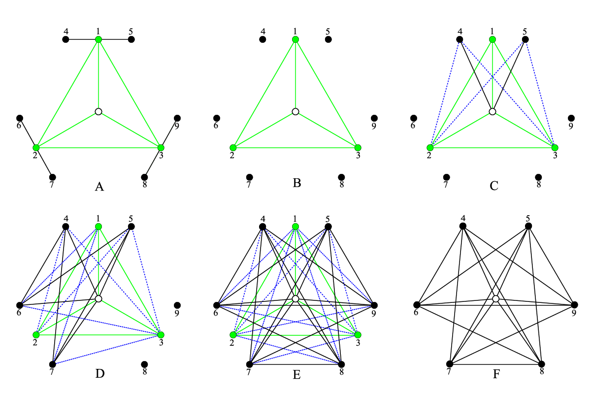
To demonstrate the above rules, let us start from the encoding graph given in FIG. 4B for the concatenated quantum code with the outer code $[[3,1,1]]$ given in FIG. 2B and the inner code $[[2,1,1]]$ given in FIG. 4A. For convenience we redraw FIG. 4B in FIG. 8A. Now from FIG. 8A we get $S_{1}=\{4,5\}$, $S_{2}=\{6,7\}$, and $S_{3}=\{8,9\}$. Deleting all the edges which connect each auxiliary vertex $i$ and vertices in $S_{i}$ (for $i=1,2,3$) results in FIG. 8B. Performing local complementation on auxiliary vertex $1$ with respect to $S_{1}=\{4,5\}$ leads to FIG. 8C, where we use dashed blue lines to show the edges that we add between output and auxiliary vertices, and solid black lines to show other edges. Performing local complementation in FIG. 8C on auxiliary vertex $2$ with respect to $S_{2}=\{6,7\}$ leads to FIG. 8D, and performing local complementation in FIG. 8D on auxiliary vertex $3$ with respect to $S_{3}=\{8,9\}$ leads to FIG. 8E. Removing all the auxiliary vertices in FIG. 8E gives FIG. 8F, which is the graph $\mathcal{G}_{c}^{\mathcal{C}_{c}}$.

From FIG. 8F one can easily see that the rule for concatenation of the classical codes given in Eq. (9) holds. In general, the outer classical code $\mathcal{C}_{\text{out}}$ is nonlinear, so we do not have the input vertices in the encoding graph of the concatenated code. However, we can still go through the whole procedure of the generalized local complementations on auxiliary vertices to obtain the graph $\mathcal{G}_{c}$. In our example this procedure is demonstrated by subgraphs of FIG. 8A through FIG. 8F without the middle white vertex.

Let $p$ be a prime number and $\mathbb{F}_{p}$ be the field of $p$ elements. A qupit is a $p$-level quantum system whose Hilbert space is represented by the orthonormal basis $\{|r\rangle:\,r\in\mathbb{F}_{p}\}=\{|0\rangle,|1\rangle,\dots,|p-1\rangle\}$. Let $\omega=e^{2\pi i/p}$ be a $p$-th root of unity. The (generalized) Pauli matrices $X$ and $Z$ are defined as follows.

It is clear that $X^{p}=Z^{p}=I$, and then we can consider the operators $X^{a}$ and $Z^{b}$ where $a,b\in\mathbb{F}_{p}$. We have $Z^{b}X^{a}=\omega^{ab}X^{a}Z^{b}$; therefore, $X^{a}Z^{b}$ and $X^{a^{\prime}}Z^{b^{\prime}}$ commute iff $ab^{\prime}-ba^{\prime}=0$ (see e.g. [20] for more details).

The group generated by the (generalized) Pauli matrices $X$ and $Z$ is $\{\omega^{c}X^{a}Z^{b}:\,a,b,c\in\mathbb{F}_{p}\}$ and is called the (generalized) Pauli group. Notice that, in the binary case ($p=2$) the Pauli group is generated by Pauli matrices $\sigma_{x}$ and $\sigma_{z}$ together with $iI$ ($i=\sqrt{-1}$).

Let $n$ be an arbitrary positive integer. For vectors $\mathbf{a}=(a_{1},\dots,a_{n})$ and $\mathbf{b}=(b_{1},\dots,b_{n})$ in $\mathbb{F}_{p}^{n}$ define

and

Again, two Pauli matrices $X^{\mathbf{a}}Z^{\mathbf{b}}$ and $X^{\mathbf{a^{\prime}}}Z^{\mathbf{b^{\prime}}}$ commute if and only if $\mathbf{a}\mathbf{b^{\prime}}-\mathbf{a^{\prime}}\mathbf{b}=0$, where $\mathbf{c}\mathbf{d}=c_{1}d_{1}+\cdots+c_{n}d_{n}$ is the usual inner product on $\mathbb{F}_{p}^{n}$.

For simplicity, a Pauli operator $X^{\mathbf{a}}Z^{\mathbf{b}}$ is denoted by the vector $(\mathbf{a}\,|\,\mathbf{b})$ of length $2n$. Thus two Pauli operators $X^{\mathbf{a}}Z^{\mathbf{b}}$ and $X^{\mathbf{a^{\prime}}}Z^{\mathbf{b^{\prime}}}$ commute iff their corresponding vectors are orthogonal with respect to the “symplectic inner product” defined by

It is easy to see that for a Pauli matrix $g=\omega^{c}X^{\mathbf{a}}Z^{\mathbf{b}}$, $g^{p}=I$. (In the case $p=2$, the statement might only be true after replacing $G$ by $ig$ in order to get $g^{2}=I$. Having this in mind, there is no true difference between the binary and non-binary case in the rest of the paper.) Therefore, the eigenvalues of $g$ are all $p$-th root of unity. In fact, if $(\mathbf{a}\,|\,\mathbf{b})$ is non-zero, then for any $i$, $\omega^{i}$ is an eigenvalue of $g$, and the multiplicity of each of these $p$ eigenvalues is equal to $p^{n-1}$ [20].

Now suppose $g_{1}=\omega^{c_{1}}X^{\mathbf{a^{1}}}Z^{\mathbf{b^{1}}},\dots,g_{k}=\omega^{c_{k}}X^{\mathbf{a^{k}}}Z^{\mathbf{b^{k}}}$ are $k$ Pauli matrices which pairwise commute and such that the subgroup generated by any $k-1$ of them does not contain the other one. Additionally, we require that the group generated by $g_{1},\dots,g_{k}$ does not contain a non-trivial multiple of identity. Since $g_{1},\dots,g_{k}$ commute, they can be diagonalized simultaneously.

This lemma is a well-known fact in the binary case [1], and a proof for the non-binary case can be found in [20].

Representing the operators $g_{1},\dots,g_{k}$ by the vectors of length $2n$, we obtain the $k\times(2n)$ matrix

of rank $k$ (because $g_{i}$ is not in the subgroup generated by the rest of $g_{j}$’s). The rows of $M$ are mutually orthogonal with respect to the symplectic inner product (see Eq. (14)).

If we consider $n$ generators, or equivalently an $n\times(2n)$ full-rank self-orthogonal matrix $M$, Lemma 1 implies that the common eigenspace of all $g_{i}$’s with eigenvalue $1$ is a one-dimensional subspace. Hence there is a unique (up to a scaler) non-zero vector $|\psi\rangle$ such that $g_{i}|\psi\rangle=|\psi\rangle$. In fact, if we consider the group $\mathcal{S}$ generated by the $g_{i}$’s, for any $h\in\mathcal{S}$ we have $h|\psi\rangle=|\psi\rangle$. The group $\mathcal{S}$, which is a maximal Abelian subgroup of the Pauli group modulo its center, is called a stabilizer group, and the state $|\psi\rangle$ is called a stabilizer state.

Notice that for a stabilizer state $|\psi\rangle$, its stabilizer group $\mathcal{S}$ is unique; however, $\{g_{1},\dots,g_{n}\}$ is just some set of generators of $\mathcal{S}$. Suppose $\{h_{1},\dots,h_{n}\}$ is another generating set of $\mathcal{S}$. Then for any $i$ there is $u_{ij}\in\mathbb{F}_{p}$ such that $h_{i}=g_{1}^{u_{i1}}\cdots g_{n}^{u_{\text{in}}}$. As a result, the vector corresponding to $h_{i}$ is equal to $(u_{i1},\dots,u_{\text{in}})M$.

The Clifford group is the normalizer of the Pauli group. In the binary case, it is well-known that the Clifford group is generated by the Hadamard gate, the phase gate, and the controlled-NOT gate [17]. A characterization of the Clifford group in the non-binary case can be found in [18].

Clifford operators are important in the stabilizer formalism because they send any stabilizer state to a stabilizer state. Suppose $|\psi\rangle$ is a stabilizer state with the stabilizer group $\mathcal{S}$. Also, let $L$ be a Clifford operator. For any $g\in\mathcal{S}$ we have $(LgL^{\dagger})L|\psi\rangle=L|\psi\rangle$. On the other hand, $LgL^{\dagger}$ is in $L\mathcal{S}L^{\dagger}$ which is a subgroup of the Pauli group since $L$ is a Clifford operator. In fact, $L\mathcal{S}L^{\dagger}$ is a maximal Abelian subgroup of the Pauli group whose corresponding stabilizer state is $L|\psi\rangle$. Therefore, Clifford operators send stabilizer states to stabilizer states.

Based on the characterization of the Clifford group [17, 18], for any two stabilizer states $|\psi\rangle$ and $|\psi^{\prime}\rangle$ there is a Clifford operator $L$ such that $L|\psi\rangle=|\psi^{\prime}\rangle$. However, it does not mean that all the stabilizer states are the same in the point of view of quantum coding theory since the operator $L$ may completely change the entanglement of a state. But if we assume that $L=L_{1}\otimes\cdots\otimes L_{n}$ is a local Clifford operator ($L$ is the tensor product of $n$ one-qupit Clifford operators), then the entanglement of $|\psi\rangle$ and $L|\psi\rangle$ are the same. Based on this idea, two stabilizer states are called “local Clifford equivalent” if they are equivalent under the action of the local Clifford group.

For the encoding circuits, we need only two Clifford operators which we describe next. Define the vector

for any $r\in\mathbb{F}_{p}$. $|\widehat{r}\rangle$ is an eigenvector of $X$, i.e., $X|\widehat{r}\rangle=\omega^{r}|\widehat{r}\rangle$, and $\{|\widehat{0}\rangle,\dots,|\widehat{p-1}\rangle\}$ is an orthonormal basis. Therefore, the operator

which is called the (generalized) Hadamard gate, is unitary. By definition $HXH^{\dagger}=Z$. Also, it is easy to see that $HZH^{\dagger}=X^{\dagger}$. Hence, $H$ is in the Clifford group. Using the above relations the proof of the following lemma is easy.

The next operator is a two-qupit gate which is called controlled-$Z$ and is defined by

We have

and thus by definition $C_{z}$ is in the Clifford group.

In the following we consider graphs whose edges are labeled by non-zero elements of $\mathbb{F}_{p}$. Considering the adjacency matrix of a graph $\mathcal{G}$, we can represent it by a symmetric matrix over $\mathbb{F}_{p}$ with zero diagonal. Suppose $G$ is such a matrix of size $n\times n$. Then $M=(I_{n}\,|\,G)$ is a full-rank $n\times(2n)$ matrix, and all of its rows are mutually orthogonal with respect to the symplectic inner product; therefore, $M$ represents a stabilizer group which corresponds to a stabilizer state. Such a stabilizer state is called a graph state, which we denote by $|{\psi}\rangle_{\mathcal{G}}$. It is well-known that any stabilizer state is local Clifford equivalent to a graph state [20], so to study the properties of stabilizer states it is sufficient to restrict ourselves to graph states.

Graph states can be generated easily using only Hadamard and controlled-$Z$ gates,

Suppose we have a graph state $|\psi\rangle_{\mathcal{G}}$ which corresponds to the graph $\mathcal{G}$ with adjacency matrix $G$, and we measure its (say) last qupit in the standard basis and get $|0\rangle$. We claim that the state after the measurement (without the measured qubit) is also a graph state whose corresponding graph is obtained from $\mathcal{G}$ by removing the last vertex. To see this fact precisely notice that since $(I_{n}\,|\,G)$ represents the stabilizer group of $|\psi\rangle_{\mathcal{G}}$, for any $i$, we have $X^{\mathbf{e}_{i}}Z^{\mathbf{g}_{i}}|\psi\rangle_{\mathcal{G}}=|\psi\rangle_{\mathcal{G}}$, where all coordinates of $\mathbf{e}_{i}$ are $0$ except the $i$-th one which is $1$, and $\mathbf{g}_{i}$ is the $i$-th row of $G$. Let

and for $1\leq i\leq n-1$ let $\mathbf{g}^{\prime}_{i}$ and $\mathbf{e}^{\prime}_{i}$ be the vectors of length $n-1$ obtained from $\mathbf{g}_{i}$ and $\mathbf{e}^{\prime}_{i}$, respectively, by deleting the last coordinate. Thus we have

As a result $X^{\mathbf{e}^{\prime}_{i}}Z^{\mathbf{g}^{\prime}_{i}}|\phi_{0}\rangle=|\phi_{0}\rangle$, which means that $|\phi_{0}\rangle$ is a stabilizer state with the stabilizer group generated by $X^{\mathbf{e}^{\prime}_{i}}Z^{\mathbf{g}^{\prime}_{i}}$, $1\leq i\leq n-1$, and the matrix representation of these generators is $(I_{n-1}\,|\,G^{\prime})$ where $G^{\prime}$ is the adjacency matrix of the graph obtained from $\mathcal{G}$ by removing its last vertex.

A CWS code $((n,K,d))_{p}$ is described by a graph $\mathcal{G}$ with $n$ vertices and edges labeled by $\mathbb{F}_{p}$, together with a classical code $\mathcal{C}$ which consists of $K$ vectors in $\mathbb{F}_{p}^{n}$. Such a code is denoted by $\mathcal{Q}=(\mathcal{G},\mathcal{C})$ [4, 5, 6].

If the classical code $\mathcal{C}$ is linear, then $\mathcal{Q}$ is a graph (stabilizer) code [4, 5, 6]. The parameters of such a graph code $\mathcal{Q}=(\mathcal{G},\mathcal{C})$ are $[[n,k,d]]_{p}$, where the classical code $\mathcal{C}$ consists of $K=p^{k}$ vectors in $\mathbb{F}_{p}^{n}$ that are indexed by the elements of $\mathbb{F}_{p}^{k}$. This $[[n,k,d]]_{p}$ graph code encodes $k$ qupits into $n$ qupits in the following way. Suppose $|\psi\rangle_{\mathcal{G}}$ is the graph state corresponding to $\mathcal{G}$. To encode a state of the form $H^{\dagger}\otimes\cdots\otimes H^{\dagger}|r_{1}\dots r_{k}\rangle$ we first find the classical codeword $\boldsymbol{\alpha}\in\mathcal{C}$ which is indexed by $r_{1}\dots r_{k}$, and then encode $H^{\dagger}\otimes\cdots\otimes H^{\dagger}|r_{1}\dots r_{k}\rangle$ into $Z^{\boldsymbol{\alpha}}|\psi\rangle_{\mathcal{G}}$ ¹¹ 1 $Z^{\boldsymbol{\alpha}}|\psi\rangle$ is usually considered as the encoded state of $|r_{1}\dots r_{k}\rangle$; however, these two codes are the same under a change of basis, and since this change of basis is applied locally, they have the same properties.. Since $\mathcal{C}$ is a linear code, it is a linear subspace of $\mathbb{F}_{p}^{n}$. We can then represent $\mathcal{C}$ by $k$ basis vectors $\boldsymbol{\alpha}_{1},\dots,\boldsymbol{\alpha}_{k}$. In this case, the state $H^{\dagger}\otimes\cdots\otimes H^{\dagger}|r_{1}\dots r_{k}\rangle$ is encoded into $Z^{r_{1}\boldsymbol{\alpha}_{1}+\cdots+r_{k}\boldsymbol{\alpha}_{k}}|\psi\rangle_{\mathcal{G}}$.

The encoding circuit of a $[[n,k,d]]$ graph code is simple, as shown in the following procedure.

For example, the encoding circuit of the graph code with a triangle graph and the classical code $\{000,111\}$ can be found in the left circuit of FIG. 5. (Notice that in the binary case $H^{\dagger}=H$.)

In general, for a graph code $\mathcal{Q}=(\mathcal{G},\mathcal{C})$ the encoding circuit can be represented graphically, and the corresponding graph is denoted by $\mathcal{G}^{\mathcal{C}}$: consider the graph $\mathcal{G}$, for any $1\leq i\leq k$ add a vertex (input vertices), attach it to the vertices of $\mathcal{G}$ (called the output vertices), and label the edge between this vertex and the $j$-th vertex of $\mathcal{G}$ by $\alpha_{ij}$. For example, FIG. 2B gives the graph $\mathcal{G}^{\mathcal{C}}$, where $\mathcal{G}$ is a triangle and $\mathcal{C}=\{000,111\}$.

To find the logical $X$ and $Z$ operators of an additive graph code we first describe the stabilizer group of the logical $|0\dots 0\rangle_{L}$ state. Notice that

and then

Therefore, all operators $Z^{\boldsymbol{\alpha}_{i}}$ are in the stabilizer group of $|0\dots 0\rangle_{L}$, and the logical $Z$ operators are described by the rows of the matrix

Since the vectors $\boldsymbol{\alpha}_{i}$ are linearly independent, without loss of generality (by a change of basis for the classical code and reordering the qupits), we may assume that the first block of the second part of this matrix is $I_{k}$. So we assume that the matrix $(I_{k}\,\,\,A)$, where $A$ is of size $k\times(n-k)$ describes a basis for $\mathcal{C}$, and the logical $Z$ operators are

Assume that

where $G_{1}$, $G_{2}$, and $B$ are of size $k\times k$, $(n-k)\times(n-k)$, and $k\times(n-k)$, respectively. Then the stabilizer group of the state $|\psi\rangle_{\mathcal{G}}$ is represented by

Now note that for any $1\leq i,j\leq k$, $(Z^{\boldsymbol{\alpha}_{i}})(X^{\textbf{e}_{j}}Z^{\textbf{g}_{j}})=\omega^{\delta_{ij}}(X^{\textbf{e}_{j}}Z^{\textbf{g}_{j}})(Z^{\boldsymbol{\alpha}_{i}})$, where $\delta_{ij}$ is the Kronecker delta function. On the other hand, the code space is invariant under $X^{\textbf{e}_{j}}Z^{\textbf{g}_{j}}$. Therefore, the logical $X$ operators can be described by the matrix

Also, it is not hard to see that the Pauli matrices corresponding to the rows of

commute with both logical $X$ and logical $Z$ operators. Therefore, the additive graph code $\mathcal{Q}$ is described by the stabilizer group

logical $Z$ operators

and logical $X$ operators

Before going into the detailed proof of the main result, we summarize our notation. Let $\mathcal{Q}=(\mathcal{G},\mathcal{C})$ be a CWS code. If $\mathcal{C}$ is linear, then $\mathcal{Q}$ is a graph code, where the code has a graphical representation denoted by $\mathcal{G}^{\mathcal{C}}$. The concatenation of two CWS quantum codes $\mathcal{Q}_{\text{in}}=(\mathcal{G}_{\text{in}},\mathcal{C}_{\text{in}})$ and $\mathcal{Q}_{\text{out}}=(\mathcal{G}_{\text{out}},\mathcal{C}_{\text{out}})$ is denoted by $\mathcal{Q}_{c}=\mathcal{Q}_{\text{in}}\sqsubset\mathcal{Q}_{\text{out}}$.

See Table I for the rest of notations.

Most of the notations have already been given in Sec. III, except for $\mathcal{G}_{\mathcal{Q}_{c}}^{\{enc\}}$ and $\mathcal{G}_{\mathcal{Q}_{c}}^{\mathcal{C}_{\text{out}}\{enc\}}$, which are discussed in Sec. II.2 and will be explained in more details in Sec. V.

References

- [1] M. A. Nielsen and I. L. Chuang, Quantum Computation and Quantum Information, Cambridge University Press, Cambridge, UK, 2000.
- [2] D. Gottesman, Ph.D. Thesis, Caltech, 1997. arXiv: quant-ph/9705052.
- [3] A. R. Calderbank, E. M. Rains, P. W. Shor, N. J. A. Sloane, IEEE Trans. Inf. Theory, 44, 1369 (1998).
- [4] A. Cross, G. Smith, J. Smolin, and B. Zeng, IEEE Trans. Inf. Theory, 55, 433 (2009).
- [5] I. Chuang, A. Cross, G. Smith, J. Smolin, and B. Zeng, J. Math. Phys. 50, 042109 (2009).
- [6] X. Chen, B. Zeng, and I. Chuang, Phys. Rev. A78, 062315 (2008).
- [7] D. Schlingemann, Quantum Information Computation, 2 (4), 307 (2002).
- [8] M. Grassl, A. Klappenecker, and M. Roetteler, Proceedings of the 2002 IEEE international symposium on information theory, 45 (2002). arXiv:quant-ph/0703112.
- [9] D. Schlingemann and R. F. Werner, Phys. Rev. A65, 012308 (2001).
- [10] M. Grassl, P. Shor, G. Smith, J. Smolin, and B. Zeng, Phys. Rev. A79, 050306(R) (2009).
- [11] M. Grassl, P. Shor, and B. Zeng, Proceedings of the 2009 IEEE international symposium on information theory, 953 (2009). arXiv:0905.0428.
- [12] E. Knill and R. Laflamme, arXiv: quant-ph/9608012.
- [13] E. Knill, R. Laflamme, and W. Zurek, arXiv: quant-ph/9610011 (1996); E. Knill, R. Laflamme, and W. Zurek, arXiv: quant-ph/9702058 (1997).
- [14] C. Zalka, arXiv: quant-ph/9612028 (1996).
- [15] D. Aharonov and M. Ben-Or, Prof. 29th Ann. ACM Symposium on Theory of Computing, pp. 176-188 (1997). arXiv: quant-ph/9611025.
- [16] M. Hein, W. Dur, J. Eisert, R. Raussendorf, M. Van den Nest, and H.J. Briegel, the Proceedings of the International School of Physics “Enrico Fermi” on “Quantum Computers, Algorithms and Chaos”, Varenna, Italy, July, (2005). arXiv:quant-ph/0602096.
- [17] J. Dehaene and B. De Moor, Phys. Rev. A68, 042318 (2003).
- [18] J. Dehaene, E. Hostens and B. De Moor, Phys. Rev. A71, 042315 (2005).
- [19] J. Dehaene, M. Van den Nest and B. De Moor, Phys. Rev. A69, 022316 (2004).
- [20] M. Bahramgiri, and S. Beigi, arXiv:quant-ph/0610267.