Effective noise reduction techniques for disconnected loops in Lattice QCD

We decompose ${\mathcal{R}}=V\,\otimes\,\mbox{colour}\,\otimes\,\mbox{spin}$ into $m$ subspaces ${\mathcal{R}}_{j}$: ${\mathcal{R}}=\oplus_{j=1}^{m}{\mathcal{R}_{j}}$. One can then set the source vectors $|\eta^{i}_{|j}\rangle$ to zero, outside of the subspace ${\mathcal{R}_{j}}$. We label the corresponding solutions as $|s^{i}_{|j}\rangle$. The solution for the all-to-all propagator is then given by the sum,

This procedure results in an $m$-fold increase in the total number of solver applications. The term ${\mathbb{1}}-\overline{|\eta\rangle\langle\eta|}$ multiplying $Q^{-1}$ in Eq. (7) only has off-diagonal entries, all of similar sizes. Therefore the off-diagonal entries of $Q^{-1}$ will determine the stochastic error of the particular observables in question. $Q^{-1}$ will exponentially decay with the spacetime distance between source and sink: spacetime components in the neighbourhood of the sink position will yield the leading contributions to the stochastic variance. Likewise the noise for spin components that are strongly coupled to each other by $Q^{-1}$, multiplied by the relevant $\Gamma$ and derivative structures, will dominate. Ideally, partitioning will black out the largest contributions to the stochastic noise. If the achieved reduction exceeds the $1/\sqrt{m}$ factor, then the computational overhead is justified. This overhead can be somewhat reduced at the expense of memory by sophisticated preconditioning techniques and/or aggressive deflation [27, 28, 29, 30, 31, 32]: the constant set-up costs of such techniques become more affordable with a larger number of right hand sides. We experimented with various patterns and combinations of colour, spin and time partitioning, see e.g. [33]. Partitioning as a stand-alone solution works very well in many situations [21, 34, 20, 22]. However, such gains are mostly eliminated once partitioning is combined with the other tricks. Time partitioning is a notable exception: in situations where only timeslice-to-all propagators are required there is no increase in the number of solves but the variance is still reduced. In the calculation of disconnected contributions to the nucleon structure it also turns out to be useful to generate the current insertion at more than one timeslice, e.g. to average the correlation with a nucleon propagating from a given source in the forward direction and the backward propagating one (which comes for free). In this case one can seed the random sources at two (or more) well separated timeslices and still gain from partitioning, without any associated overhead.

The stochastic noise from terms that are close to the diagonal is accompanied by larger amplitudes than terms that are far off the diagonal, see Eq. (7) and the discussion in Sec. 2.1 above. Hence the cancellation of near-diagonal noise requires a comparatively larger number of estimates. The HPE aims at eliminating some of the near-diagonal noise contributions by exploiting the ultra-locality of the action. Thus it cannot be generalized for instance to the Neuberger action [35].

We rewrite the fermionic matrix as,

The HPE is based on the observation that one can expand,

where $k\geq 1$. For distances between source and sink consisting of more than $k$ links, the first term on the right hand side does not contribute since $D$ only connects nearest spacetime neighbours. Therefore, $M^{-1}_{xy}=[(\kappa D)^{k}M^{-1}]_{xy}$ for sufficiently large source and sink separations. However, at finite $N$, $\{\mathrm{E}[M^{-1}]\}_{xy}\neq\{\mathrm{E}[(\kappa D)^{k}M^{-1}]\}_{xy}(=\{(\kappa D)^{k}\mathrm{E}[M^{-1}])\}_{xy})$, where the variance of the latter estimate of $M^{-1}_{xy}$ is reduced. This was for instance exploited in [25]. In some cases additional powers of $D$ can be gained due to the $\Gamma$ structure of the creation and annihilation operators.

Here we study closed loops, i.e. $x=y$. Obviously, only even powers of $D$ contribute to $\mathrm{Tr}\,(M^{-1}\Gamma)$, where $\Gamma\in\{{\mathbb{1}},\gamma_{\mu},\sigma_{\mu\nu},\gamma_{\mu}\gamma_{5},\gamma_{5}\}$. We can write, $\mathrm{Tr}\,(M^{-1}{\mathbb{1}})=2\kappa\,\mathrm{Tr}\,{\mathbb{1}}+\kappa^{k}\mathrm{Tr}\,(D^{k}M^{-1})$, where the first term can be computed trivially. In the other cases, $\mathrm{Tr}\,(M^{-1}\Gamma)=\kappa^{k}\mathrm{Tr}\,(D^{k}M^{-1}\Gamma)$. For the Wilson action, $k=8$ for $\Gamma\in\{\gamma_{\mu}\gamma_{5},\gamma_{5}\}$ and $k=4$ otherwise. For the Sheikholeslami-Wohlert action [36], $k=2$. The lowest non-vanishing terms have been calculated analytically [23] and can be computed and corrected for exactly (unbiased noise subtraction) [23, 37, 5]. We limit ourselves to the highest vanishing order ($k=4$ or $k=8$ for the Wilson action), where such subtraction is not necessary. In this case the computational overhead of the HPE is small, such that this substitution can easily be combined with the TSM that we explain below.

It has been noticed long ago [38] that solvers typically converge to the correct result within an accuracy of the size of the stochastic error after a relatively small number of iterations. Practitioners have therefore sometimes relaxed the requirement on the residual when solving for stochastic sources. This is not unproblematic since it introduces a systematic bias that will be invisible on one configuration but might very well affect the result obtained on a sample of, say, 200 configurations. We label the result obtained after $n_{\rm t}$ solver iterations by $|s_{(n_{\rm t})}^{i}\rangle$, where omitting the subscript means convergence within numerical accuracy. We can now factorize:

The above equation is an exact linear decomposition of $Q^{-1}$ and the algorithm used to calculate both parts is well defined. Due to these properties and the fact that the $|\eta^{i}\rangle$ with $i\leq N_{1}$ are uncorrelated with those for $i>N_{1}$, the resulting estimate is unbiased. Ideally, one will generate a large number $N_{1}\gg N_{2}$ of relatively cheap estimates at small $n_{\rm t}$ and then remove the bias by correcting with a small number $N_{2}$ of expensive solutions to machine precision. This method can easily be combined with all the other methods described here. It is possible to tune the two parameters $N_{1}/N_{2}$ and $n_{\rm t}$ that enter the algorithm to the point of minimal variance at fixed computer time in a relatively inexpensive and straightforward way. This is discussed in A.

In some sense the underlying philosophy of TSM is similar to estimating the cheap first term within the HPE Eq. (12) with many random sources and the expensive second term with only a few sources. However, iterative solvers like the CG converge faster than the HPE. Moreover, TSM is applicable to any fermion action, not only to ultra-local ones, and efficient for any quark mass. TSM can be combined with HPE, see Sec. 2.5 below.

To check our implementation of the method we compared the exact result for $(M^{-1})_{x,y}^{s_{1}c_{1},s_{2}c_{2}}$, where $s_{1}c_{1}$ denotes the spin and colour indices, $x=(0,0,0,3)$ and $y=(i,0,0,3)$, $i=0\ldots 10$, with an estimate obtained from Eq. (13). We indeed find consistency within errors for different $n_{\rm t}$, $N_{1}$ and $N_{2}$. For example, for $n_{\rm t}=5$, $N_{1}=5500$, $N_{2}=300$, $i=1$, $s_{1}=s_{2}=1$, $c_{1}=c_{2}=2$, $\mathrm{E}[M^{-1}_{n_{c}}]=(0.0300(7),-0.0014(7))$, compared to the exact result of $(0.0302\ldots,-0.0010\ldots)$.

In A we also demonstrate that the TSM can be generalized to other solvers, by employing BiCGstab2. However, the smooth convergence of CG, that is relatively independent of the random source and gauge configuration, is a clear advantage when it comes to deciding on a TSM parameter set. Moreover, in the CG case the combination with the truncated eigenmode acceleration bears less computational overhead and is compatible with even-odd preconditioning (see below). We emphasize however that the converged solutions $|s^{i}\rangle$ within Eq. (13) can be obtained by using any efficient solver. In particular, there is no need to employ the same solver as that used for obtaining the truncated solutions $|s^{i}_{(n_{t})}\rangle$. The truncated solver of course needs to be the same for $i>N_{1}$ as that used for $i\leq N_{1}$.

We define the $n_{\rm e}$ smallest (real) eigenvalues $q_{i}$ of $Q$ and the corresponding orthonormal eigenvectors $|u_{i}\rangle$, $i=1,\ldots,n$:

These can for instance be calculated by means of the parallel implicitly restarted Arnoldi method (IRAM) with Chebychev acceleration [39] or by Ritz methods [40].

We can now approximate [39],

However, this estimate is biased. We define the projection operator ${\mathbb{P}}_{n_{\rm e}}$, onto the complement of the space spanned by these $n_{\rm e}$ eigenvectors,

Projecting the stochastic sources onto the orthogonal complement,

yields the new unbiased estimate [25],

where a left projection of $|s_{\perp}^{i}\rangle$ is not necessary since $[Q,{\mathbb{P}}_{n_{\rm e}}]=0$ and thus ${\mathbb{P}}_{n_{\rm e}}Q\,{\mathbb{P}}_{n_{\rm e}}=Q\,{\mathbb{P}}_{n_{\rm e}}$. The above estimate will usually have a reduced variance. Note that in the literature exact point-to-all propagators have also been combined with a truncated low eigenmode all-to-all calculation to achieve smaller gauge errors (low mode averaging) [41, 42].

A nice side effect of TEA lies in the acceleration of the solver, by deflation [43, 27, 29, 31, 44, 32]. The condition number of the projected operator $Q\,{\mathbb{P}}_{n_{\rm e}}$ and therefore the number of solver iterations are reduced. Within some algorithms like the CG the fact that the projector commutes with the operator $Q$ guarantees that the Krylov subspace remains confined within the orthogonal complement. So in these cases no further intermediate projections are necessary to fully exploit the potential of deflation.

Note that while the number of undeflated solver iterations increases like $1/m_{\rm PS}^{2}$ at small quark masses, the efficiency of the eigenvalue calculation remains the same. Unfortunately, at small $m_{\rm PS}$, one would like to increase the linear lattice extent $L\propto 1/m_{\rm PS}$. In this case, the rank of the deflation space in the worst case will increase like $n_{\rm e}\propto L^{4}\propto Va^{4}$. Depending on the volume required this may or may not become a serious problem. The volume scaling of stochastic methods is somewhat more favourable: the number of estimates needs to be adjusted at most like $\sqrt{V}a^{2}$ (this can be somewhat reduced by partitioning). From these considerations it becomes evident that the optimal choices of $n_{\rm e}$ and $N$ strongly depend on the volume, the quark mass and the lattice spacing. The same holds for the algorithm where a deflated CG can outperform a (deflated) BiCGstab2, in particular when combined with the truncated solver method.

Obviously, it is also possible to decompose $M$, rather than the Hermitian operator $Q=\gamma_{5}M$ of Eq. (15), into eigenmodes [45]: $M|r_{i}\rangle=\lambda_{i}|r_{i}\rangle$. However, in this case we end up with a biorthonormal system $\langle\ell_{i}|r_{j}\rangle=\delta_{ij}$, where the left eigenvectors $|\ell_{i}\rangle$ will differ from the right eigenvectors: $\langle\ell_{i}|M=\langle\ell_{i}|\lambda_{i}$. One can now decompose,

It can easily be seen that due to the property $M^{\dagger}=\gamma_{5}M\gamma_{5}$, $\tilde{\lambda}_{i}:=\lambda_{i}^{*}$ is an eigenvalue whenever $\lambda_{i}$ is an eigenvalue, with a left eigenvector $\langle\tilde{\ell}_{i}|=\langle r_{i}|\gamma_{5}$ and a right eigenvector $|\tilde{r}_{i}\rangle=\gamma_{5}|\ell_{i}\rangle$. The advantage of this decomposition is that the eigenvectors are independent of the quark mass and the eigenvalues at different $\kappa$ values are trivially related to each other. This follows from the structure Eq. (11). In this article we will not pursue this alternative eigenmode decomposition any further. However, the decomposition of $M^{-1}$ might converge better in some channels than that of $Q^{-1}$ and vice versa. While this biorthogonal approach is incompatible with deflating the CG solver, it would be the natural starting point for BiCG solvers.

Partitioning can trivially be combined with the other three methods. However some notes are in place with respect to combinations of HPE, TSM and TEA. Within the HPE a left-multiplication of the estimate $\mathrm{E}[Q^{-1}]$ with $D^{k}$ is essential since we have defined $M^{-1}=Q^{-1}\gamma_{5}$. A right-multiplication would involve $\gamma_{5}D\gamma_{5}=D^{\dagger}$. The easiest way of implementing HPE is to multiply the solution vectors with $(\kappa D)^{k}$, prior to any application of smearing functions or contractions but after TEA and TSM.

Within Eq. (18) only the projected source vectors appear. Hence after the projection, Eq. (17),

the original noise vectors $|\eta^{i}\rangle$ can be discarded.

The overhead from the projection can be significant when combined with the TSM, Eq. (13), where the large number of estimates $N_{1}$ implies a large number of projections and the small number of solver iterations $n_{\rm t}$ indicates that not much computer time will be spent between these projections. The projection overhead can be reduced by restricting the computation of the inner products to the partitioning subspace: many components of $|\eta^{i}\rangle$ might have been set to zero if the partitioning method was used. This saving cannot be obtained at the sink. Fortunately, $[{\mathbb{P}}_{n_{\rm ev}},Q]=0$, such that the solutions $|s^{i}_{\perp}\rangle$ remain within the orthogonal complement and no second projection is necessary, provided the residual of the solver is chosen sufficiently small!

Obviously the residual will not be small for the truncated solutions, which therefore one would wish to project back into the orthogonal complement (before application of the $D$ operator within the HPE). Fortunately, the (even-odd preconditioned) CG algorithm never leaves the orthogonal subspace: in this case, such an additional projection is never necessary, even if the solver is not run to convergence. Neither is such a left projection strictly required for solvers without this property, as long as the precision of the part that is run to convergence is sufficiently large. In this case, the $N_{1}$ biased estimates will pick up some unwanted low mode contributions that will however be corrected for by the $N_{2}$ estimates of the bias. This might or might not increase the stochastic errors.

For completeness we mention that domain decomposition techniques have been suggested in the literature [46, 47]. These can easily be combined with TSM and TEA too, as can the so-called one-end-trick [48, 49, 50]. We remark that if a bosonic representation is employed [46, 51], estimating $M^{\dagger}M=Q^{2}$ instead of $Q$, then the TSM can in principle be substituted by a quasi heatbath strategy [52].

We study combinations of the variance reduction techniques outlined above, using configurations provided by the Wuppertal group: these are $n_{\rm f}=2+1$ dynamical configurations with $V=16^{3}\times 32$ lattice points, generated using a Symanzik improved gauge action and a stout-link improved (rooted) staggered fermion action. The lattice spacing is fairly coarse, $a^{-1}\approx 1.55$ GeV, while the spatial extent is around $2$ fm. Further details can be found in [53]. For the valence quarks we use the Wilson action with $\kappa=0.166$, $0.1675$ and $0.1684$, corresponding to pseudoscalar masses of about $600$, $450$ and $300$ MeV, respectively. The analysis is performed on 326 configurations at $\kappa_{\rm loop}=0.166$, 167 configurations at $\kappa_{\rm loop}=0.1675$ and $152$ configurations at $\kappa_{\rm loop}=0.1684$, where $\kappa_{\rm loop}$ refers to the $\kappa$ value of the disconnected loop. Our main results are obtained using the CG solver with even-odd preconditioning. However, results obtained with BiCGstab2 are given in A. The code used throughout is a modified version of Chroma [54, 55, 56].

We wish to calculate nucleon structure observables. For this purpose a nucleon will be created at some initial time $t_{0}$ and destroyed at a later time $t_{\rm f}\gg t_{0}$, with a current inserted at some intermediate time $t$. This is illustrated in Fig. 1. The disconnected loop $\mathrm{Tr}\,(M^{-1}\Gamma)$ within the right diagram of the figure will be calculated with stochastic all-to-all techniques and can subsequently be combined with the nucleon two-point function, calculated in the standard point-to-all way, on a configuration by configuration basis.

A preliminary picture of how well the variance reduction techniques work can be obtained by studying the zero-momentum projected disconnected loop $\sum_{\mathbf{x}}\mathrm{Tr}\,(M^{-1}_{xx}\Gamma)$ alone, where $x=(\mathbf{x},t)$. With the exception of $\Gamma={\mathbb{1}}$, expectation values of these loops over many configurations vanish, due to the discrete charge and parity symmetries of QCD. However, the expectation value of the correlation between loop and proton (with a momentum injected or with a specified helicity) can be non-zero. Likewise, with the exception of trivial cases such as $\mathrm{Im}\,\mathrm{Tr}\,(M^{-1}\gamma_{5})=0$, the loops will not vanish on single configurations. Using the Euclidean spacetime convention $\{\gamma_{\mu},\gamma_{\nu}\}=2\delta_{\mu\nu}$, $\gamma_{5}=\gamma_{1}\gamma_{2}\gamma_{3}\gamma_{4}$, we are interested in evaluating $\mathrm{Re}\,\mathrm{Tr}\,(M^{-1}{\mathbb{1}})$, $\mathrm{Im}\,\mathrm{Tr}\,(M^{-1}\gamma_{\mu})$, $\mathrm{Im}\,\mathrm{Tr}\,(M^{-1}\sigma_{\mu\nu})=\mathrm{Re}\,\mathrm{Tr}\,(M^{-1}\gamma_{\mu}\gamma_{\nu})$ for $\mu\neq\nu$, $\mathrm{Re}\,\mathrm{Tr}\,(M^{-1}\gamma_{\mu}\gamma_{5})$ and $\mathrm{Im}\,\mathrm{Tr}\,(M^{-1}\gamma_{5})$.

We investigate the reduction in computer time of optimized stochastic estimates, relative to the situation without the use of any improvement techniques (except for time partitioning: all disconnected loops are calculated on one timeslice only). We state all costs in terms of the average real computer time required on a Pentium 4 PC for one solver application (unimproved estimate), where we account for all overheads of the improvement methods. We also ran the parallelized code on IBM p6 and Opteron clusters as well as on BlueGene/L and BlueGene/P systems. The overall efficiencies of matrix-vector multiplies and global sums depend on the architecture, however, the gain factors defined below are not significantly affected.

We define the gain as the ratio,

taken at fixed real computer time. $\mathrm{var}$ denotes the variance between stochastic estimates on a given gauge configuration, $\mathrm{E}_{0}$ and $\mathrm{E}_{\rm imp}$ stand for the unimproved and improved estimated, respectively.

We start by investigating the TSM at the heaviest quark mass, $\kappa_{\rm loop}=0.166$. Within TSM the combination $\mathrm{Tr}\,(M^{-1}\Gamma)$ is obtained as an average over $N_{1}$ truncated solutions $|s^{i}_{(n_{\rm t})}\rangle$: $\langle\eta^{i}|\gamma_{5}\Gamma|s^{i}_{(n_{\rm t})}\rangle$. This value is then corrected by $N_{2}\ll N_{1}$ estimates of the resulting bias, see Eq. (13). The faster the truncated estimate as a function of $n_{\rm t}$ approaches the estimate obtained at full convergence, the better the method will work. In this study we only consider currents of local quark bilinears, where we use the $\Gamma$ conventions of [54]. We observe very satisfactory convergence rates for all the 16 possible $\Gamma$ structures. In Fig. 2 we illustrate this for the even/odd preconditioned CG solver for the worst case ($\Gamma=\mathbb{1}$) and for the best case ($\Gamma=\gamma_{3}\gamma_{5}$). Note, however, that the unimproved estimate of $\Gamma=\mathbb{1}$ is already very precise to start with. Convergence at this $\kappa$ value is reached after $n_{\rm conv}\approx 480$ CG iterations.

Applying TSM involves making choices for $n_{\rm t}$ and for $N_{1}/N_{2}$. We detail our optimization procedure in A. This systematic tuning results in similar amounts of computer time being spent on the truncated estimate as on estimating the bias. In particular we find $N_{1}/N_{2}\approx n_{\rm conv}/n_{\rm t}$. Performing this optimization on a single configuration appears sufficient since the variance is not much affected if $n_{\rm t}$ and $N_{1}/N_{2}$ are changed by $20\,\%$. Fluctuations between configurations turn out to be smaller than this value.

In Table 1 we display the optimized parameters at $\kappa_{\rm loop}=0.166$ for a representative choice of $\Gamma$ structures (scalar, vector, tensor, pseudoscalar and axial vector), together with the approximate fixed cost gains, Eq. (21). These factors vary between 5 and 10. In a real production run one would not wish to generate new sets of optimized estimates for each $\Gamma$ structure or observable one is interested in. Fortunately, with the still tolerable exception of $\Gamma={\mathbb{1}}$, $n_{\rm t}$ and $N_{1}/N_{2}$ exhibit only a mild $\Gamma$ dependence such that similar overall gains can still be achieved with just one parameter set.

TSM can trivially be combined with the hopping parameter expansion. At $\kappa_{\rm loop}=0.166$ the gains from applying a stand-alone HPE are almost as big as those from the TSM. However, the HPE does not work well for $\Gamma=\mathbb{1}$, see Fig. 3. Both methods aim at removing noisy short range contributions from the estimates. Clearly, the gain from combining the two methods will be smaller than the product of the two isolated gains. However, the separation of long and short range is organized differently. The HPE only works for ultra-local actions and explicitly removes terms up to a particular lattice hopping radius. It will be less convergent and hence less effective at very light quark masses. The TSM is more generally applicable and separates short range modes from long range ones, but this is done within the Krylov space of the solver. When combining HPE with TSM, the reduced variances of the truncated estimates result in larger optimal $n_{\rm t}$ values. The constant computational overhead per solve of the additional $D$ applications also pushes $n_{\rm t}$ towards larger values. Table 1 demonstrates that the combined gain of these two methods at $\kappa_{\rm loop}=0.166$ can be as large as a factor of $30$.

Having tested the method at $\kappa_{\rm loop}=0.166$, where $m_{\rm PS}\approx 600$ MeV, we also use it to calculate the disconnected loop at $\kappa_{\rm loop}=0.1675$ and at $\kappa_{\rm loop}=0.1684$, corresponding to pseudoscalars masses of approximately $450$ MeV and $300$ MeV, respectively. The resulting gains are displayed in Table 2. While the TSM performance is very independent of the quark mass, the HPE becomes less effective at lighter masses, in agreement with our expectation. Still, even at the lightest quark mass, the combined gains range from factors of 6 (for $\Gamma=\mathbb{1}$) up to 19 (for $\Gamma=\gamma_{3}\gamma_{5}$).

At light quark masses where the HPE becomes less effective, the low eigenmode contributions to hadronic observables might become more dominant [39, 41, 42, 25]. To study this effect, we deflate the lowest eigenmodes at the lightest pseudoscalar mass. As expected, this accelerates the solver [43, 26, 27, 28, 29, 30, 31, 44, 32]. We display a typical residual, as a function of the number of CG iterations, without deflation and deflating the lowest 5, 10, 20 and 50 modes of the Hermitian Wilson-Dirac operator in Fig. 4.

The optimized TSM parameters at $\kappa_{\rm loop}=0.1684$ for combining TSM with HPE as well as for combining TSM with HPE and the TEA of the lowest 20 eigenmodes are shown in Table 3. The faster rate of convergence of the deflated solver leads to smaller $n_{\rm t}$ values and therefore to larger $N_{1}/N_{2}$ ratios when TSM is combined with TEA. When normalized to the real cost of generating 300 unimproved stochastic estimates, all gain factors increase by more than a factor of two, and this in spite of one quarter of the time being spent on generating and projecting onto the eigenvectors. However, this factor can fully be attributed to the acceleration of the solver: while there exist observables where stochastic errors decrease when applying the TEA [39, 41, 25], for the quark loops that we investigate here this is not the case, at least not at pseudoscalar masses above 300 MeV. We observe a break-even between TSM+HPE+TEA(${\mathbb{P}}_{20}$) and TSM+HPE when matching the cost of approximately 100 estimates, as can be seen in the last row of the table. In lattice simulations we will encounter gauge errors from the Monte Carlo time series, in addition to the errors from the stochastic estimates on single configurations, discussed here. This interplay is studied below.

When calculating averages over configurations, the stochastic errors $\sigma_{\rm stoch}$, that are defined in Eq. (8), should be smaller than say half of the final Monte Carlo errors $\sigma_{\rm tot}$. However, making $\sigma_{\rm stoch}$ unnecessarily small can be a waste of computer time that would be more wisely spent on analysing more configurations or realizing additional source positions. We start to study this balance of errors by computing expectation values over configurations for the disconnected loops. In Sec. 4 below we will then calculate the three point functions that are of physical interest.

We remark that the (zero momentum projected) gauge average $\langle\mathrm{Re}\,\mathrm{Tr}\,(M^{-1}{\mathbb{1}})\rangle_{c}$ will have a non-trivial value, while $\langle\mathrm{Re}\,\mathrm{Tr}\,(M^{-1}\gamma_{\mu}\gamma_{5})\rangle_{c}=0$. We first assess the impact of low mode deflation. In Fig. 5 we display the number of CG iterations until convergence $n_{\rm conv}$ for several random sources on different gauge configurations. Without deflation, reducing the quark mass from $m_{\rm PS}\approx 600$ MeV ($\kappa=0.166$, black symbols of the left figure) to $m_{\rm PS}\approx 300$ MeV ($\kappa=0.1684$, red symbols of the right figure), we find $n_{\rm conv}$ to grow from about 500 to 1800 iterations. This approximately four-fold increase is consistent with the expected $1/m_{\rm PS}^{2}$ behaviour of the condition number of $M$ (we solve for $Q^{2}=M^{\dagger}M$). Deflating 5 eigenmodes ($\mathbb{P}_{5}$) at $\kappa=0.1675$ reduces the required number of iterations by one third (red versus blue symbols of the left figure) and deflating 20 modes at $\kappa=0.1684$ results in a two third reduction (red versus blue symbols of the right figure). We observe variations of $n_{\rm conv}$ between and within configurations that increase with decreasing quark mass, as has been investigated quantitatively in [57]. Deflating the lowest modes vastly reduces the variance in $n_{\rm conv}$. Clearly, the TSM parameter tuning benefits from this stabilization.

We now average our improved estimates over $n$ configurations, where we employ TSM, HPE and, at the lightest $\kappa$ value, TEA with a projection onto the 20 lowest modes. In addition, we calculate up to 100 unimproved estimates on each configuration. The results as functions of the real computer time spent, in units of the cost of one unimproved estimate, i.e. of one solve, are displayed in Table 4, for $\Gamma=\mathbb{1}$ and $\Gamma=\gamma_{j}\gamma_{5}$, where we average over the three possible $j$-directions. The total errors $\sigma_{\rm tot}$ are displayed in brackets, followed by their respective lower bounds, as given by the stochastic errors $\sigma_{\rm stoch}$.

For $\Gamma=\mathbb{1}$, even at the cost equivalent of six standard estimates, the gauge errors still dominate over the improved stochastic errors. Therefore, there is little point in exceeding this number. On the given ensemble, the same error can be obtained using 25 to 50 standard estimates, suggesting a five-fold saving in computer time. However, this is somewhat misleading since, by just increasing the number of gauge configurations by a factor of 1.6, the same error can be obtained, employing six unimproved estimates. It should be noted that the error balance could in principle look differently, once the loop is correlated with a nucleon propagator, within a three point function. Moreover, the stochastic error will become more relevant on large volumes. At the lightest $\kappa$ value, due to the overhead of setting up TEA, the cost of the improved estimates will always exceed the number 6. In fact, as can also be seen from Table 4, TEA only turns out to be a worthwhile enterprise for a cost equivalent bigger than 90. Hence, unless the eigenvectors have been generated anyway, for instance to enable low mode averaging [41] for the two point functions or for the calculation of other current insertions, TEA is best omitted for $\Gamma=\mathbb{1}$.

The picture for the axial current containing $\Gamma=\gamma_{j}\gamma_{5}$ is different: here at the cost equivalent of 100 standard estimates, the stochastic error still accounts for one quarter of the total error and the gain of applying the improved method is in all cases more than four-fold. This advantage should increase further at larger volumes. Note that the reductions of the stochastic errors alone, for the scalar and axial cases, are consistent with the results of Table 2 that were obtained on a single configuration.

Based on these results, we decide to invest the cost equivalent of 100 even/odd preconditioned CG solves into the TSM/HPE/(TEA) estimation of the axial loop and of 6 CG solves into the estimation of the scalar loop. Note that for the calculation of a standard point-to-all baryonic two-point correlation function usually 12 such solves are required, and even more sources if a variational basis is used to optimize the creation operator. We display the resulting stochastic errors $\Delta_{\rm stoch}$ on single configurations at $\kappa_{\rm loop}=0.166$ in Fig. 6. This graphical representation again makes it evident that even for this low-cost setting the stochastic errors are much smaller than the gauge noise. The larger error bars on the right of the figures correspond to unimproved $\Delta_{\rm stoch}$ values, obtained at the same cost. After application of the improvement methods, the stochastic errors are so small that nothing extra can be gained from increasing the number of stochastic sources (and solves) beyond these moderate values.

We now apply our methods to the calculation of observables of phenomenological interest, namely of $\Delta q$ and $\langle N|\bar{q}q|N\rangle$. The contribution to the nucleon spin $\Delta q$ is defined through the matrix element (in Minkowski space notation),

where $m_{N}$ denotes the mass of the nucleon $N$ and $s_{\mu}$ its spin ($s_{\mu}^{2}=-1$). $\Delta q$ and $\langle N|\bar{q}q|N\rangle$ are extracted from the ratios of three-point functions to two-point functions (at zero momentum):

For the scalar matrix element we use, $\Gamma_{\rm 2pt}=\Gamma_{\rm unpol}:=(1+\gamma_{4})/2$ and $\Gamma_{\rm loop}=\mathbb{1}$. For $\Delta q$ we calculate the difference between two polarizations: $\Gamma_{\rm 2pt}=\gamma_{j}\gamma_{5}\Gamma_{\rm unpol}$ and $\Gamma_{\rm loop}=\gamma_{j}\gamma_{5}$, where we average over all three possible $j$-orientations. The spin projection operators along the $j$-axis read, $P_{\uparrow\downarrow}=\frac{1}{2}(\mathbb{1}\pm i\gamma_{j}\gamma_{5})$, so that in this case, $\Gamma_{\rm 2pt}=-i(P_{\uparrow}-P_{\downarrow})\Gamma_{\rm unpol}$, where we have traded a factor $i$ against taking the real part, rather than the imaginary part, of the nominator in Eq. (23). The variance of the above expression is reduced by explicitly using the fact that $\mathrm{Im}\,\mathrm{Tr}\,(M^{-1}{\mathbb{1}})=\mathrm{Im}\,\mathrm{Tr}\,(M^{-1}\gamma_{j}\gamma_{5})=0$.

The two-point function of the zero momentum projected proton with sink and source spinor indices $\alpha$ and $\beta$ is given by,

where we have set $t_{0}=0$. This can be constructed from standard point-to-all quark propagators [6]. Note that for $q=u,d$ there are additional connected contributions $R^{\rm con}$, which we have not calculated. We combine the three $\kappa_{\rm loop}$ values with $\kappa_{\rm 2pt}=0.166$ and 0.1675.

In the limit of large times, $t_{\rm f}\gg t\gg 0$, in the axial case,

The prefactor two comes from taking the difference between two opposite polarizations rather than fixing one polarization. We note that this result will be in a lattice scheme and still needs to be multiplied by a renormalization factor of $\mathcal{O}(1)$, for a translation into the $\overline{MS}$ scheme. In the scalar case, $\langle N|\bar{q}q|N\rangle$ is defined as the connected contribution only and can thus be obtained by subtracting $\langle 0|\bar{q}q|0\rangle=-\sum_{\mathbf{x}}\mathrm{Re}\left\langle\mathrm{Tr}\,(M^{-1}(\mathbf{x},t;\mathbf{x},t)\right\rangle_{c}$ from Eq. (23). We will label the disconnected contributions to these two matrix elements as, $\Delta q^{\rm dis}$ and $\langle N|\bar{q}q|N\rangle^{\rm dis}$, respectively. In the case of the strange quark, $\Delta s=\Delta s^{\rm dis}$ and $\langle N|\bar{s}s|N\rangle=\langle N|\bar{s}s|N\rangle^{\rm dis}$.

We calculate the disconnected loop on only one timeslice $t=3\approx 0.38\,\mathrm{fm}/a$. Having the operator inserted close to the source ($t_{0}=0$) reduces the statistical errors but care must be taken that contributions from excited states are suppressed so that Eq. (25) still holds. Following [25], we use Wuppertal smearing on top of APE smeared links at the source and sink for both the three point and two point functions. In Fig. 7 we display the effective mass,

as a function of the time. This shows that with our choice of smearing parameters the excited state contributions are not significant at $t=3$. Hence, in the symmetric situation, $t_{\rm f}=6$, such contributions should be negligible. This is even more so since the statistical error will be much bigger than that of the two point function at $t=3$. The consistency of this assumption can be checked by varying $t_{\rm f}\geq 4$.

In Fig. 8 we display finite time estimates of the matrix elements $\langle N|\bar{q}q|N\rangle^{\rm dis}$ and $\Delta q^{\rm dis}$ in the lattice scheme, for different final times $t_{\rm f}$ at $\kappa_{\rm loop}=\kappa_{\rm 2pt}=0.166$. This value approximately corresponds to the mass of the strange quark. The stochastic estimates of the loops were generated using time partitioning ($t=3$), TSM and HPE, at the cost of 6 even/odd preconditioned CG solves for the scalar and at the cost of 100 such solves for the axial current. Our analysis of the two point function above suggests that finite $t$ systematics should be small, relative to the statistical errors at $t_{\rm f}=6$. Indeed, all $t_{\rm f}\geq 4$ data are consistent with a constant. We conservatively quote the $t_{\rm f}=6$ values as our final results. We realized all six $\kappa_{\rm loop}\in\{0.166,0.1675,0.1684\}$ and $\kappa_{\rm 2pt}\in\{0.166,0.1675\}$ combinations where the lightest $\kappa_{\rm loop}$ value corresponds to $m_{\rm PS}\approx 300$ MeV. The five combinations that are not shown result in the same general picture, with larger statistical errors. For the two point function we do not realize the lightest $\kappa$ value since, without low mode averaging, this turns out to be very noisy.

In Table 5 we display improved and conventional stochastic estimates of the scalar matrix elements (obtained at $t_{0}=0$, $t=3$ and $t_{\rm f}=6\approx 0.76\,\mathrm{fm}/a$), for all our $\kappa$ combinations. The fixed cost reductions, due to TSM and HPE, in the relative errors are small and do by far not match the gain factors that we obtained in Sec. 3 for the disconnected loops alone. The noise is dominated by taking the correlation with the two point function. For the precision of the disconnected loop to be matched by that of the two point function, the latter needs to be evaluated for multiple source points, eventually in combination with low mode averaging [41]. We note that one does not encounter any computational overhead in calculating the disconnected loop at more than one timeslice. As long as these are sufficiently separated, the stochastic errors will not increase significantly.

In Table 6 we display the same information as in Table 5, for $\Delta q^{\rm dis}$ in the lattice scheme. In this case, at the cost equivalent of 100 estimates (90 estimates at $\kappa_{\rm loop}=0.1684$), the gains of applying TSM and HPE in terms of computer time, relative to time partitioning alone, are about ten-fold. The reductions in error are close to those displayed in Table 4 for the disconnected loop alone. This channel is not yet limited by the accuracy of the two point function but of course also in this case statistics could be increased by averaging over multiple baryon sources and over forward as well as backward propagation.

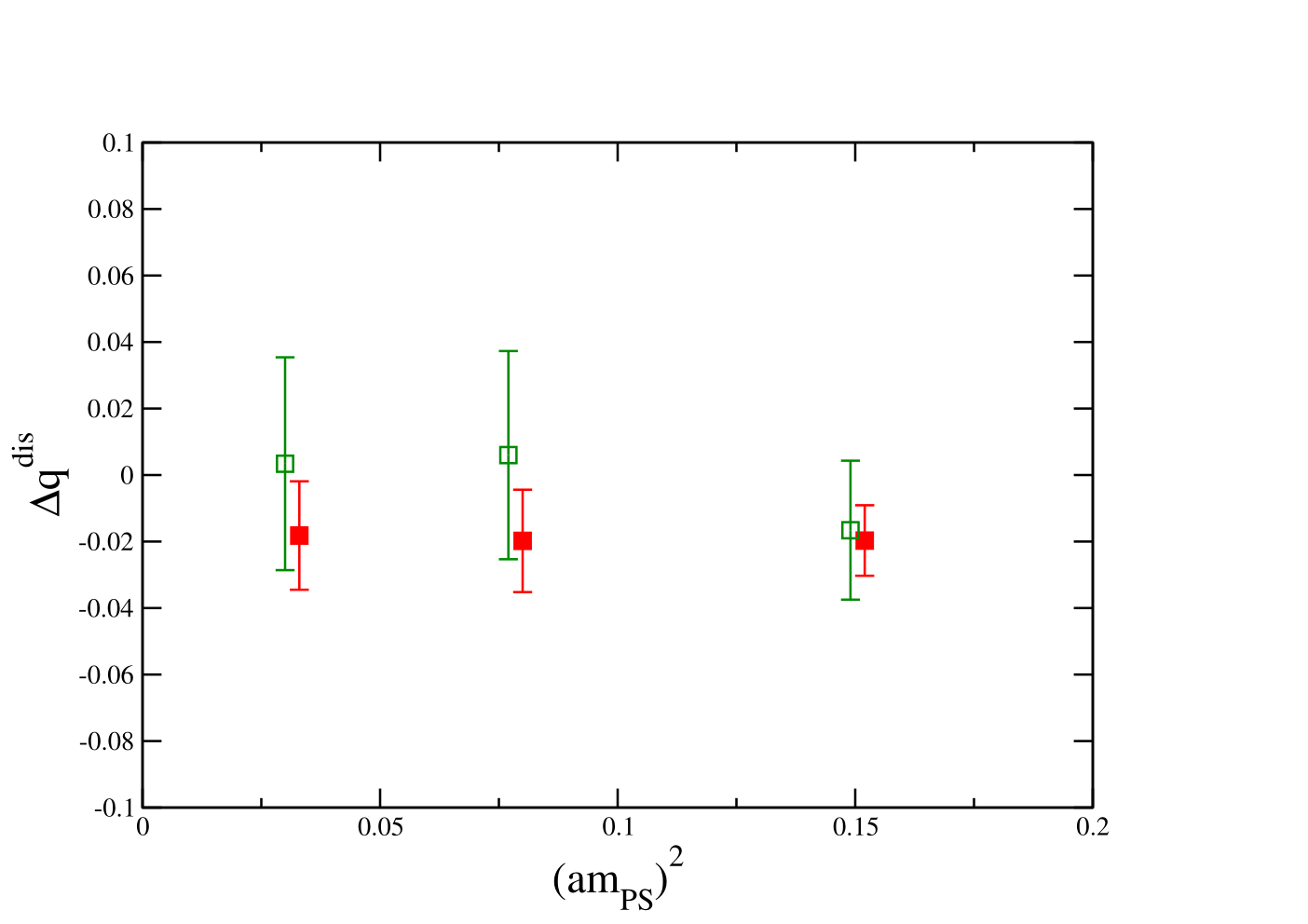
In Fig. 9 we display our final $t_{\rm f}=6$ results for the two matrix elements. In neither case do we observe any significant dependence on the valence quark mass, varying this from $m_{\rm PS}\approx 600$ MeV down to 450 MeV, or on the loop quark mass, reducing $m_{\rm PS}\approx 600$ MeV (strange quark mass) to $m_{\rm PS}\approx 300$ MeV. We find $\Delta s=-0.020(11)$ at the heavier proton mass and $\Delta s=-0.017(21)$ at the lighter mass value, while the scalar matrix elements are somewhat larger than one. Note that the lattice results presented here are unrenormalized. However, based on perturbative two loop results [58], albeit with different sea quark and gluon actions, we would not expect $\Delta s$ to change by more than a factor of 0.7 after a translation into the $\overline{MS}$ scheme.

References

- [1] K. Jansen, C. Michael and C. Urbach [ETM Collaboration], The meson from Lattice QCD, Eur. Phys. J. C 58 (2008) 261, arXiv:0804.3871 [hep-lat].
- [2] J. Bulava, R. Edwards, K. J. Juge, C. J. Morningstar and M. J. Peardon [Hadron Spectrum Collaboration], Multi-hadron operators with all-to-all quark propagators, PoS (LATTICE 2008) 124, arXiv:0810.0730 [hep-lat].
- [3] S. Aoki, M. Fukugita, K-I. Ishikawa, N. Ishizuka, K. Kanaya, Y. Kuramashi, Y. Namekawa, M. Okawa, K. Sasaki, A. Ukawa, T. Yoshié [CP-PACS Collaboration], Lattice QCD calculation of the meson decay width, Phys. Rev. D 76 (2007) 094506, arXiv:0708.3705 [hep-lat].
- [4]
J. M. Zanotti,
Investigations of hadron structure on the lattice,
PoS (LATTICE 2008) 007,
arXiv:0812.3845 [hep-lat]. - [5] M. Deka T. Streuer, T. Doi, S. J. Dong, T. Draper, K.-F. Liu, N. Mathur and A. W. Thomas, Moments of nucleon’s parton distribution for the sea and valence quarks from Lattice QCD, Phys. Rev. D 79 (2009) 094502, arXiv:0811.1779 [hep-ph].
- [6] T. DeGrand and C. DeTar, Lattice methods for quantum chromodynamics, (World Scientific, Singapore, 2006).
- [7] A. Airapetian et al. [HERMES Collaboration], Measurement of parton distributions of strange quarks in the nucleon from charged-kaon production in deep-inelastic scattering on the deuteron, Phys. Lett. B 666 (2008) 446, arXiv:0803.2993 [hep-ex].
- [8] S. L. Zhu, G. Sacco and M. J. Ramsey-Musolf, Recoil order chiral corrections to baryon octet axial currents and large QCD, Phys. Rev. D 66 (2002) 034021, arXiv:hep-ex/0201179.
- [9] D. de Florian, R. Sassot, M. Stratmann and W. Vogelsang, Extraction of spin-dependent parton densities and their uncertainties, Phys. Rev. D 80 (2009) 034030, arXiv:0904.3821 [hep-ph].
- [10] A. Airapetian et al. [HERMES Collaboration], Precise determination of the spin structure function of the proton, deuteron and neutron, Phys. Rev. D 75 (2007) 012007, arXiv:hep-ex/0609039.
- [11] A. Frommer, V. Hannemann, B. Nöckel, T. Lippert and K. Schilling, Accelerating Wilson fermion matrix inversions by means of the stabilized biconjugate gradient algorithm,” Int. J. Mod. Phys. C 5 (1994) 1073, arXiv:hep-lat/9404013.
- [12] S. Collins, G. S. Bali and A. Schäfer, Disconnected contributions to hadronic structure: a new method for stochastic noise reduction, PoS (LATTICE 2007) 141, arXiv:0709.3217 [hep-lat].
- [13] G. S. Bali, S. Collins and A. Schäfer, Hunting for the strangeness content of the nucleon, PoS (LATTICE 2008) 161, arXiv:0811.0807 [hep-lat].
- [14]
K. G. Wilson,
Quarks on a lattice,
in Proceedings of
Methods in Field Theory, Les Houches 1975, Amsterdam 1976, 261;
Quarks on a lattice, or, the colored string model, Phys. Rept. 23 (1976) 331. - [15] K. Bitar, A. D. Kennedy, R. Horsley, S. Meyer and P. Rossi, The QCD finite temperature transition and hybrid Monte Carlo, Nucl. Phys. B 313 (1989) 348.
- [16] M. F. Hutchinson, A stochastic estimator of the trace of the influence matrix for Laplacian smoothing splines, Commun. Statist.-Simula. 18(3) (1989) 1059.
- [17] S. J. Dong and K.-F. Liu, Quark loop calculations, Nucl. Phys. B (Proc. Suppl.) 26 (1992) 353.
- [18] S. Bernardson, P. McCarty and C. Thron, Monte Carlo methods for estimating linear combinations of inverse matrix entries in Lattice QCD, Comput. Phys. Commun. 78 (1993) 256.
- [19] R. Babich, R. Brower, M. Clark, G. Fleming, J. Osborn and C. Rebbi, Strange quark contribution to nucleon form factors, PoS (LATTICE 2007) 139, arXiv:0710.5536 [hep-lat].
- [20] W. Wilcox, Noise methods for flavor singlet quantities, arXiv:hep-lat/9911013.
- [21] J. Viehoff, N. Eicker, S. Güsken, H. Hoeber, P. Lacock, T. Lippert, G. Ritzenhöfer, K. Schilling, A. Spitz, P. Ueberholz [SESAM Collaboration], Improving stochastic estimator techniques for disconnected diagrams, Nucl. Phys. B (Proc. Suppl.) 63 (1998) 269, arXiv:hep-lat/9710050.
- [22]
A. O’Cais, J. Foley, K. Jimmy Juge, M. Peardon, S. M. Ryan and J. I. Skullerud
[TrinLat Collaboration],
Improving algorithms to compute all elements of the lattice quark
propagator,
Nucl. Phys. B (Proc. Suppl.) 140 (2005) 844,
arXiv:hep-lat/0409069;
Practical all-to-all propagators for Lattice QCD, Comput. Phys. Commun. 172 (2005) 145, arXiv:hep-lat/0505023. - [23] C. Thron, S. J. Dong, K. F. Liu and H. P. Ying, Padé- estimator of determinants, Phys. Rev. D 57 (1998) 1642, arXiv:hep-lat/9707001.
- [24] C. Michael, M. S. Foster and C. McNeile [UKQCD Collaboration], Flavour-singlet pseudoscalar and scalar mesons, Nucl. Phys. B (Proc. Suppl.) 83 (2000) 185, arXiv:hep-lat/9909036.
- [25]
G. S. Bali, T. Düssel, T. Lippert, H. Neff, Z. Prkacin and K. Schilling
[SESAM Collaboration],
String breaking with dynamical Wilson fermions,
Nucl. Phys. B (Proc. Suppl.) 140 (2005) 609,
arXiv:hep-lat/0409137;
G. S. Bali, T. Düssel, T. Lippert, H. Neff and K. Schilling [SESAM Collaboration], Observation of string breaking in QCD, Phys. Rev. D 71 (2005) 114513, arXiv:hep-lat/0505012. - [26] T. A. DeGrand and U. M. Heller [MILC Collaboration], Witten-Veneziano relation, quenched QCD, and overlap fermions, Phys. Rev. D 65 (2002) 114501, arXiv:hep-lat/0202001.
- [27] R. B. Morgan and W. Wilcox, Deflated iterative methods for linear equations with multiple right-hand sides, arXiv:math-ph/0405053.
- [28] M. Lüscher, Local coherence and deflation of the low quark modes in Lattice QCD, JHEP 0707 (2007) 081, arXiv:0706.2298 [hep-lat].
- [29] A. Stathopoulos and K. Orginos, Computing and deflating eigenvalues while solving multiple right hand side linear systems in Quantum Chromodynamics, arXiv:0707.0131 [hep-lat].
- [30] J. Brannick, R. C. Brower, M. A. Clark, J. C. Osborn and C. Rebbi, Adaptive multigrid algorithm for Lattice QCD, Phys. Rev. Lett. 100 (2008) 041601, arXiv:0707.4018 [hep-lat].
- [31] W. M. Wilcox, Deflation methods in fermion inverters, PoS (LATTICE 2007) 025, arXiv:0710.1813 [hep-lat].
- [32] H. Tadano, Y. Kuramashi and T. Sakurai, Application of preconditioned block BiCGGR to the Wilson-Dirac equation with multiple right-hand sides in Lattice QCD, arXiv:0907.3261 [hep-lat].
- [33] C. Ehmann and G. S. Bali, --mixing with improved stochastic estimators, PoS (LATTICE 2008) 114, arXiv:0903.2947 [hep-lat].
- [34] S. Güsken, Flavor singlet phenomena in Lattice QCD, arXiv:hep-lat/9906034.
- [35] H. Neuberger, Exactly massless quarks on the lattice, Phys. Lett. B 417 (1998) 141, arXiv:hep-lat/9707022.
- [36] B. Sheikholeslami and R. Wohlert, Improved continuum limit lattice action for QCD with Wilson fermions, Nucl. Phys. B 259 (1985) 572.
- [37] N. Mathur and S. J. Dong, Study of stochastic estimates of quark loops with unbiased subtraction, Nucl. Phys. B (Proc. Suppl.) 119 (2003) 401, arXiv:hep-lat/0209055.
- [38] N. Eicker, U. Glässner, S. Güsken, H. Hoeber, T. Lippert, G. Ritzenhöfer, K. Schilling, G. Siegert. A. Spitz, P. Ueberholz and J. Viehoff [SESAM Collaboration], Evaluating sea quark contributions to flavour-singlet operators in lattice QCD, Phys. Lett. B 389 (1996) 720, arXiv:hep-lat/9608040.
- [39] H. Neff, N. Eicker, T. Lippert, J. W. Negele and K. Schilling, On the low fermionic eigenmode dominance in QCD on the lattice, Phys. Ref. D 64 (2001) 114509, arXiv:hep-lat/0106016.
- [40] T. Kalkreuter and H. Simma, An accelerated conjugate gradient algorithm to compute low lying eigenvalues: a study for the Dirac operator in Lattice QCD, Comput. Phys. Commun. 93 (1996) 33 arXiv:hep-lat/9507023.
- [41] T. A. DeGrand and S. Schäfer, Improving meson two-point functions in Lattice QCD, Comput. Phys. Commun. 159 (2004) 185, arXiv:hep-lat/0401011.
- [42] L. Giusti, P. Hernández, M. Laine, P. Weisz and H. Wittig, Low-energy couplings of QCD from current correlators near the chiral limit, JHEP 04 (2004) 013, arXiv:hep-lat/0402002.
- [43]
P. de Forcrand,
Progress on lattice QCD algorithms,
Nucl. Phys. B (Proc. Suppl.) 47 (1996) 228,
arXiv:hep-lat/9509082. - [44] D. Darnell, R. B. Morgan and W. Wilcox, Deflated GMRES for systems with multiple shifts and multiple right-hand sides, Linear Algebra Appl. 429 (2008) 2415, arXiv:0707.0502 [math-ph].
- [45] I. Hip, T. Lippert, H. Neff, K. Schilling and W. Schroers, Instanton dominance of topological charge fluctuations in QCD?, Phys. Rev. D 65 (2002) 014506, arXiv:hep-lat/0105001.
- [46] C. Michael and J. Peisa [UKQCD Collaboration], Maximal variance reduction for stochastic propagators with applications to the static quark spectrum, Phys. Rev. D 58 (1998) 034506, arXiv:hep-lat/9802015.
- [47] T. Burch and C. Hagen, Domain decomposition improvement of quark propagator estimation, Comput. Phys. Commun. 176 (2007) 137, arXiv:hep-lat/0607029.
- [48] M. Foster and C. Michael [UKQCD Collaboration], Quark mass dependence of hadron masses from Lattice QCD, Phys. Rev. D 59 (1999) 074503, arXiv:hep-lat/9810021.
- [49] C. McNeile and C. Michael [UKQCD Collaboration], Decay width of light quark hybrid meson from the lattice, Phys. Rev. D 73 (2006) 074506, arXiv:hep-lat/0603007.
- [50] P. A. Boyle, J. M. Flynn, A. Jüttner, C. Kelly, H. Pedroso de Lima, C. M. Maynard, C. T. Sachrajda and J. M. Zanotti [UKQCD Collaboration], The pion’s electromagnetic form factor at small momentum transfer in full Lattice QCD, JHEP 0807 (2008) 112, arXiv:0804.3971 [hep-lat].
- [51] A. Duncan and E. Eichten, Improved pseudofermion approach for all-point propagators, Phys. Rev. D 65 (2002) 114502, arXiv:hep-lat/0112028.
- [52]
Monte Carlo quasi-heatbath by approximate inversion,
Phys. Rev. E 59 (1999) 3698,
arXiv:cond-mat/9811025. - [53] Y. Aoki, Z. Fodor, S. D. Katz and K. K. Szabo, The equation of state in Lattice QCD: with physical quark masses towards the continuum limit, JHEP 01 (2006) 089, arXiv:hep-lat/0510084.
- [54] R. G. Edwards [LHP Collaboration] and B. Joó [UKQCD Collaboration], The Chroma software system for Lattice QCD, Nucl. Phys. B (Proc. Suppl.) 140 (2005) 832, arXiv:hep-lat/0409003.
- [55] C. McClendon, Optimized Lattice QCD kernels for a Pentium 4 cluster, Jlab preprint (2001) JLAB-THY-01-29, http://www.jlab.org/edwards/qcdapi/reports/dslash_p4.pdf.
- [56] P.A. Boyle, http://www.ph.ed.ac.uk/paboyle/bagel/Bagel.html (2005).
- [57] L. Del Debbio, L. Giusti, M. Lüscher, R. Petronzio and N. Tantalo, Stability of Lattice QCD simulations and the thermodynamic limit, JHEP 0602 (2006) 011, arXiv:hep-lat/0512021.
- [58] A. Skouroupathis and H. Panagopoulos, Two-loop renormalization of vector, axial-vector and tensor fermion bilinears on the lattice, Phys. Rev. D 79 (2009) 094508, arXiv:0811.4264 [hep-lat].
- [59] R. Babich, R. Brower, M. Clark, G. Fleming, J. Osborn and C. Rebbi, Strange quark content of the nucleon, PoS (LATTICE 2008) 160, arXiv:0901.4569 [hep-lat].
- [60] M. Fukugita, Y. Kuramashi, M. Okawa and A. Ukawa, Proton spin structure from Lattice QCD, Phys. Rev. Lett. 75 (1995) 2092, arXiv:hep-lat/9501010.
- [61] S. J. Dong, J. F. Lagae and K.-F. Liu, Flavor singlet from Lattice QCD, Phys. Rev. Lett. 75 (1995) 2096, arXiv:hep-ph/9502334.
- [62] S. Güsken, J. Viehoff, N. Eicker, T. Lippert, K. Schilling, A. Spitz and T. Struckmann [TL Collaboration], Flavor singlet axial vector coupling of the proton with dynamical Wilson fermions, Phys. Rev. D 59 (1999) 114502, arXiv:hep-lat/9901009.
- [63] G. S. Bali, S. Collins and A. Schäfer [QCDSF Collaboration], Strangeness and charm content of the nucleon, PoS (LAT 2009) 149, arXiv:0911.2407 [hep-lat].