Finite element computation of absorbing boundary conditions for time-harmonic wave problems

Denis Duhamel Corresponding author: Corresponding author, duhamel@lami.enpc.fr. Address: Université Paris-Est, UR Navier,
Ecole des Ponts ParisTech,
6 et 8 Avenue Blaise Pascal,
Cité Descartes, Champs sur Marne,
77455 Marne la Vallée, cedex 2, France
Tel: 33 1 64 15 37 28
Fax: 33 1 64 15 37 41
email : duhamel@lami.enpc.fr Tien-Minh Nguyen Address: Université Paris-Est, UR Navier,
Ecole des Ponts ParisTech,
6 et 8 Avenue Blaise Pascal,
Cité Descartes, Champs sur Marne,
77455 Marne la Vallée, cedex 2, France
Tel: 33 1 64 15 37 28
Fax: 33 1 64 15 37 41
email : duhamel@lami.enpc.fr

Abstract

This paper proposes a new method, in the frequency domain, to define absorbing boundary conditions for general two-dimensional problems. The main feature of the method is that it can obtain boundary conditions from the discretized equations without much knowledge of the analytical behavior of the solutions and is thus very general. It is based on the computation of waves in periodic structures and needs the dynamic stiffness matrix of only one period in the medium which can be obtained by standard finite element software. Boundary conditions at various orders of accuracy can be obtained in a simple way. This is then applied to study some examples for which analytical or numerical results are available. Good agreements between the present results and analytical solutions allow to check the efficiency and the accuracy of the proposed method.

Keywords:

Absorbing boundary conditions, waveguide, finite element, periodic medium.

Number of pages : 47

Number of figures : 17

1 Introduction

Wave problems in unbounded media can occur in many applications in mechanics and engineering such as in acoustics, solid mechanics, electromagnetics, etc. It is well known that analytical solutions for such problems are available only for some special cases. On the contrary, numerical methods can be applied to many complex problems. Physically, for problems in infinite domains, the energy is produced by sources in the region to be analyzed and must escape to infinity. For methods solving the problem on a bounded domain like the finite element method, it introduces the difficulty of an artificial boundary to get a bounded domain. This boundary must be such that the energy crosses it without reflection and special conditions must be specified at the artificial boundary to reproduce this phenomena. Generally, these can be classified into local or global boundary conditions. With a global condition all degrees of freedom (dofs) on the boundary are coupled while a local condition connects only neighboring dofs.

The first global method which has been used for solving such problems was the boundary element method. This method is well adapted for infinite domains and is described in numerous classical textbooks like [1, 2, 3, 4, 5]. It consists in solving an equation on the boundary of the domain only and the radiation conditions are taken into account analytically. It also reduces the dimension of the problem to a surface in 3D and to a curve in 2D decreasing thus the size of the linear problem to solve. However, the final problem involves full matrices which are also generally non symmetrical. It is also mainly limited to linear problems and to homogeneous domains or otherwise one has to introduce special and complex techniques to deal with non linear or non homogeneous situations. There are also singularities in the integrals which need special attention for the numerical integrations. So this method is interesting and has been extensively used but it can lead to heavy computations when the number of degrees of freedom increases. More information on such techniques can be found in the historical and review papers [6, 7].

In the other approaches, the computational domain is truncated at some distance and boundary conditions are imposed at this artificial boundary. These conditions at finite distance must simulate as closely as possible the exact radiation condition at infinity. An approach leading to a global boundary condition is the Dirichlet to Neumann (DtN) mapping proposed by [8, 9] and in an earlier version by [10, 11]. It consists in dividing the domain into a finite part containing the sources and an infinite domain of simple shape. The solution in the infinite domain is solved analytically, for example by series expansions, and an exact impedance relation is obtained on the boundary between the finite and infinite domains. This relation links the variable and its normal derivative on the whole boundary. The DtN mapping is thus non local and every node on the boundary is connected to all other nodes. This gives a full matrix for the nodes of the boundary which partially destroys the sparse matrix of the FEM and increases substantially the computing resources needed to get the solution. The solution has to be found in the exterior domain by analytical or numerical methods. When the analytical solution can be found, it is generally under the form of a series expansion. The number of terms in the expansion must be sufficient for an accurate solution which can lead to heavy computations. Developments of the method can be found in [12, 13]. An application to the case of wave scattering in plates is also found in [14].

The other methods are local and the condition at a node involves only neighboring nodes which make them less demanding in computing resources and much easier to implement in a finite element code but also less accurate. A first possibility of such approaches is the use of infinite elements as proposed by [15, 16, 17, 18, 19]. It consists in developing special elements with a behavior at infinity reflecting that of analytical solutions obtained for the same type of problems. For wave problems, it involves complex-valued basis functions with outwarding propagation wave-like behavior in the radial direction. The elements were further developed by [20] to considered other coordinate systems such as expansions in prolate coordinates. This method is interesting but the inclusion of infinite elements requires the development of special elements and these elements can depend on decay parameters which have to be accurately chosen. A review of these methods has been proposed by [21].

In the perfectly matched layer proposed by [22, 23], originally for electromagnetic waves, an exterior layer of finite thickness is introduced around the bounded domain. The absorption in this domain is increasing as we move towards the exterior such that outgoing waves are absorbed before reaching the exterior truncation boundary. The number of elements in the layer, its thickness, the variation of the absorption properties have to be carefully chosen to optimize the efficiency of the method. This efficiency is better for a layer with a large thickness but this can lead to a significant increase in the number of elements in the finite element model. Various developments of the method can be found in [24] and its optimization in [25]. Otherwise, various classes of absorbing boundary conditions were also developed by [26]. They consist in the numerical approximation of differential operators on the boundary. For instance, examples of the application of Bayliss-Turkel conditions are presented by [27]. However, the more accurate boundary conditions involve high order derivatives on the boundary which are difficult to implement in the finite element method [28]. Finally, it was proved by [25, 29] that, in fact, the perfectly matched layer and the absorbing boundary conditions were closely connected. The Helmholtz equation was also solved with these two boundary conditions by [30] and these conditions were compared and optimized to minimize the reflection. Other boundary conditions involving only second order derivatives have also been proposed. They introduce auxiliary variables and systems of equations on the boundary which lead to high order boundary conditions, see [31] for a review of such non-reflecting boundary (NRBC) methods. They were mainly developed for acoustic problems but in [32] a local boundary condition for elastic waves has been proposed. In [33] an impedance boundary condition in new coordinates was developed for the convected Helmholtz equation. For fluid dynamic problems, [34] developed Lagrange multipliers for imposing various absorbing boundary conditions for cases where the type and the number of boundary conditions can change, for instance as the flow changes from subsonic to supersonic regimes and its direction varies with time. A general review of the methods described in the precedent paragraphs for various dynamic, acoustic and wave propagation problems can be found in [35, 36, 37, 38]. Comparisons are also made between the different methods.

In the present study, another local method is proposed. This method works on discrete systems directly, in contrast with many existing absorbing boundary conditions which are written on the continuous differential equations and discretized after. The principle of the method is to compute wave propagations in groups of elements near the boundary from the dynamic stiffness matrix of these elements. Then, a boundary condition is obtained for cancelling the reflected waves. This condition is finally written as an impedance boundary condition relating the force and displacement degrees of freedom on the boundary. The approach is based on the waveguide theory proposed by [39, 40, 41] and is used to determine absorbing boundary conditions at the truncation boundary of 2D periodic media. Only information related to one period, obtained from any standard FE software (the discrete stiffness and mass matrices and the nodal coordinates) are required to formulate the method. The advantage is that it can be applied to media with various complex behaviors.

This paper is outlined as follows. In section 2, the methodology for determining absorbing boundary conditions for periodic media is described. Then, a discussion for the application of the method to general media is proposed. In section 3, a simple application is proposed to show the results of the method in a case where detailed computations can be done. In section 4, two examples of finite element computations in acoustics and elastodynamics are presented. They allow to check the efficiency and accuracy of the proposed method for more complex cases. Finally, the paper is closed with some conclusions.

2 Absorbing boundary conditions

We suppose that we want to solve a mechanical problem on an infinite domain exterior to the bounded domain $\Omega_{int}$ (see figure 1). The infinite domain is approximated by the finite domain $\Omega$ which is exterior to $\Omega_{int}$ and is limited by the exterior boundary $\Gamma_{ext}$ . We are looking for a solution with radiating condition at infinity which means that the solution should be outgoing near the boundary $\Gamma_{ext}$ . Near this exterior boundary the solution can be seen as composed of incident waves denoted $A_{+}$ and reflected waves $A_{-}$ . For a perfectly absorbing boundary, one should have $A_{-}=0$ . In fact this condition is very difficult to implement in the numerical solutions of such problems. Indeed, only the global solution is easily computed but the decomposition into incident and reflected waves is difficult to obtain. The problem is thus to find an appropriate boundary condition to impose on the exterior boundary to finally get $A_{-}\approx 0$ on the solution. To be easily included in a finite element model the searched boundary condition should be local and the condition at a node of the boundary should involve only neighboring nodes.

The approach proposed in this paper consists in studying this problem by first considering the case of periodic media. For this case, positive and negative waves and their amplitudes $A_{+}$ and $A_{-}$ can be computed by the method presented below. Then an exact boundary condition can be formulated for a half-plane boundary. It is further shown how this condition can be approximated by a local condition on the boundary. As homogeneous media are special cases of periodic media, the method presented here applies also to homogeneous media. Before considering the general case, a simple example for the Klein Gordon equation will be presented.

2.1 A simple example

Consider first the stationary Klein Gordon equation given by

\frac{d^{2}u}{dx^{2}}+(k^{2}-m^{2})u=0

(1)

where $u$ is the solution and $k$ , $m$ are real parameters. This equation is discretized with linear two nodes elements such that

u(\xi)=u_{1}N_{1}(\xi)+u_{2}N_{2}(\xi)

(2)

where $N_{1}(\xi)=(1-\xi)/2$ , $N_{2}(\xi)=(1+\xi)/2$ , $u_{1}$ and $u_{2}$ are the values of the function at the two nodes of the element. The discretization of the first and second parts of relation (1) leads, for an element of length $l$ , to the matrices

\mathbf{k}=-\frac{1}{l}\left[\begin{array}[]{cc}1&-1\\ -1&1\end{array}\right]\ \ \ \ \ \mathbf{m}=\frac{l}{6}\left[\begin{array}[]{cc}2&1\\ 1&2\end{array}\right]

(3)

and the dynamic stiffness matrix of one element is given by

\mathbf{d}=-\frac{1}{l}\left[\begin{array}[]{cc}1&-1\\ -1&1\end{array}\right]+\frac{l}{6}(k^{2}-m^{2})\left[\begin{array}[]{cc}2&1\\ 1&2\end{array}\right]

(4)

Waves of propagating constant $e^{\mu}$ are such that

	$\displaystyle u_{2}$	$\displaystyle=$	$\displaystyle e^{\mu}u_{1}$		(5)
	$\displaystyle f_{2}+e^{\mu}f_{1}$	$\displaystyle=$	$\displaystyle 0$		(6)

leading in an element to

e^{2\mu}d_{12}+(d_{11}+d_{22})e^{\mu}+d_{21}=0

(7)

where $d_{ij}$ are the components of the matrix $\mathbf{d}$ . Taking into account the symmetries in the matrix $\mathbf{d}$ , this yields

e^{2\mu}+2\frac{d_{11}}{d_{12}}e^{\mu}+1=0

(8)

whose solutions are

e^{\mu_{\pm}}=-\frac{d_{11}}{d_{12}}\pm\sqrt{(\frac{d_{11}}{d_{12}})^{2}-1}\\

(9)

with

\frac{d_{11}}{d_{12}}=-\frac{1-l^{2}(k^{2}-m^{2})/3}{1+l^{2}(k^{2}-m^{2})/6}

(10)

For $l^{2}(k^{2}-m^{2})<<1$ , one gets, at first order,

e^{\mu_{\pm}}\approx 1\pm il\sqrt{k^{2}-m^{2}}

(11)

meaning

\mu_{\pm}\approx\pm il\sqrt{k^{2}-m^{2}}

(12)

There are thus two waves in an element, such that

\left[\begin{array}[]{c}u_{+}\\ f_{+}\end{array}\right]=\left[\begin{array}[]{c}1\\ d_{11}+e^{\mu_{+}}d_{12}\end{array}\right]\ \ and\ \ \left[\begin{array}[]{c}u_{-}\\ f_{-}\end{array}\right]=\left[\begin{array}[]{c}1\\ d_{11}+e^{\mu_{-}}d_{12}\end{array}\right]

(13)

and the general solution is given by

\left[\begin{array}[]{c}u\\ f\end{array}\right]=a_{+}\left[\begin{array}[]{c}u_{+}\\ f_{+}\end{array}\right]+a_{-}\left[\begin{array}[]{c}u_{-}\\ f_{-}\end{array}\right]

(14)

The condition for only outgoing waves is thus $a_{-}=0$ on the right boundary and $a_{+}=0$ on the left boundary leading respectively to the conditions

	$\displaystyle f/u$	$\displaystyle=$	$\displaystyle f_{+}/u_{+}\ \ on\ the\ right$
	$\displaystyle f/u$	$\displaystyle=$	$\displaystyle f_{-}/u_{-}\ \ on\ the\ left$		(15)

The condition in the first case is

$\displaystyle f/u$	$\displaystyle=$	$\displaystyle d_{11}+e^{\mu_{+}}d_{12}$	(16)
	$\displaystyle=$	$\displaystyle d_{11}+\left(-\frac{d_{11}}{d_{12}}+\sqrt{(\frac{d_{11}}{d_{12}})^{2}-1}\right)d_{12}$
	$\displaystyle=$	$\displaystyle\sqrt{d_{11}^{2}-d_{12}^{2}}$
	$\displaystyle=$	$\displaystyle\sqrt{-(k^{2}-m^{2})+\frac{1}{12}((k^{2}-m^{2})l)^{2}}$
	$\displaystyle=$	$\displaystyle i\sqrt{k^{2}-m^{2}}\sqrt{1-\frac{1}{12}(k^{2}-m^{2})l^{2}}$
	$\displaystyle\approx$	$\displaystyle i\sqrt{k^{2}-m^{2}}$	(17)

In the second case, one gets

f/u=d_{11}+e^{\mu_{-}}d_{12}\approx-i\sqrt{k^{2}-m^{2}}

(18)

We recognize approximations of the classical absorbing boundary conditions which have been obtained here directly from the discretized equations. Compared to the classical boundary condition on the right (and exact in this case) $f/u=i\sqrt{k^{2}-m^{2}}$ , the relative error is $\sqrt{1-\frac{1}{12}(k^{2}-m^{2})l^{2}}$ which depends mainly on the size of the element relatively to the wavelength. The present boundary condition has been obtained entirely from the discrete matrices without any knowledge of the analytical solution of the problem.

To estimate the reflection coefficient created by such a boundary condition consider an incident wave $Ae^{i\sqrt{k^{2}-m^{2}}x}$ on the boundary. A reflected wave $RAe^{-i\sqrt{k^{2}-m^{2}}x}$ is created. The total solution and its associated force are given by

	$\displaystyle u(x)$	$\displaystyle=$	$\displaystyle Ae^{i\sqrt{k^{2}-m^{2}}x}+RAe^{-i\sqrt{k^{2}-m^{2}}x}$
	$\displaystyle f(x)$	$\displaystyle=$	$\displaystyle Ai\sqrt{k^{2}-m^{2}}e^{i\sqrt{k^{2}-m^{2}}x}-RAi\sqrt{k^{2}-m^{2}}e^{-i\sqrt{k^{2}-m^{2}}x}$		(19)

Writing the boundary condition (16), for instance by taking the boundary at $x=0$ , yields

\frac{f(0)}{u(0)}=\frac{1-R}{1+R}=\sqrt{1-\frac{1}{12}(k^{2}-m^{2})l^{2}}

(20)

So the reflection coefficient is finally given by

	$\displaystyle R$	$\displaystyle=$	$\displaystyle\frac{1-\sqrt{1-\frac{1}{12}(k^{2}-m^{2})l^{2}}}{1+\sqrt{1-\frac{1}{12}(k^{2}-m^{2})l^{2}}}$		(21)
		$\displaystyle\approx$	$\displaystyle\frac{1}{48}(k^{2}-m^{2})l^{2}$		(21)

This coefficient is low and of second order when $\sqrt{k^{2}-m^{2}}l<<1$ .

2.2 General impedance boundary condition

In this section we present the general outline of the method before starting a more rigorous developement in the following section. So, to extend the precedent example to more general cases, consider a vector function $\mathbf{u}(x,y)$ and a force vector $\mathbf{f}(x,y)$ acting on a line parallel to the $y$ axis as in figure 2. They can be decomposed by a Fourier transform as

	$\displaystyle\mathbf{u}(x,y)=\frac{1}{(2\pi)^{2}}\int_{-\infty}^{+\infty}\int_{-\infty}^{+\infty}\mathbf{u}(k_{x},k_{y})e^{i(k_{x}x+k_{y}y)}dk_{x}dk_{y}$
	$\displaystyle\mathbf{f}(x,y)=\frac{1}{(2\pi)^{2}}\int_{-\infty}^{+\infty}\int_{-\infty}^{+\infty}\mathbf{f}(k_{x},k_{y})e^{i(k_{x}x+k_{y}y)}dk_{x}dk_{y}$		(22)

Let us suppose that $\mathbf{u}$ is solution of a linear operator

L(\mathbf{u})=\sum_{n=0}^{n=N}\sum_{\alpha_{1}+\alpha_{2}=n}\mathbf{a}_{\alpha_{1}\alpha_{2}}\frac{\partial^{n}\mathbf{u}}{\partial x^{\alpha_{1}}\partial y^{\alpha_{2}}}=0

(23)

In the Fourier domain, this relation yields

\left(\sum_{n=0}^{n=N}\sum_{\alpha_{1}+\alpha_{2}=n}\mathbf{a}_{\alpha_{1}\alpha_{2}}(ik_{x})^{\alpha_{1}}(ik_{y})^{\alpha_{2}}\right)\mathbf{u}(k_{x},k_{y})=0

(24)

For a given value of $k_{y}$ , the precedent relation has non zero solutions for $k_{x}$ such that the determinant

\left|\sum_{n=0}^{n=N}\sum_{\alpha_{1}+\alpha_{2}=n}\mathbf{a}_{\alpha_{1}\alpha_{2}}(ik_{x})^{\alpha_{1}}(ik_{y})^{\alpha_{2}}\right|=0

(25)

Let us denote by $k_{j}^{+}$ the $n_{+}$ positive solutions such that $Re(k_{j}^{+})<0$ or $Re(k_{j}^{+})=0$ and the energy flux is directed towards positive values of x. We denote by $k_{j}^{-}$ the other solutions. We have the decomposition

\mathbf{u}(x,k_{y})=\sum_{j=1}^{j=n_{+}}a_{j}^{+}\mathbf{u}_{j}^{+}e^{ik^{+}_{j}x}+\sum_{j=1}^{j=n_{-}}a_{j}^{-}\mathbf{u}_{j}^{-}e^{ik^{-}_{j}x}

(26)

In the same way, for the force components

\mathbf{f}(x,k_{y})=\sum_{j=1}^{j=n_{+}}a_{j}^{+}\mathbf{f}_{j}^{+}e^{ik^{+}_{j}x}+\sum_{j=1}^{j=n_{-}}a_{j}^{-}\mathbf{f}_{j}^{-}e^{ik^{-}_{j}x}

(27)

where $\mathbf{f}_{j}^{+}$ and $\mathbf{f}_{j}^{-}$ are the force components respectively associated to $\mathbf{u}_{j}^{+}$ and $\mathbf{u}_{j}^{-}$ . If the boundary is such that only positive waves exists at proximity, one has

	$\displaystyle\mathbf{u}(0,k_{y})$	$\displaystyle=$	$\displaystyle\sum_{j=1}^{j=n_{+}}a_{j}^{+}\mathbf{u}_{j}^{+}=\mathbf{U}^{+}\mathbf{a}^{+}$
	$\displaystyle\mathbf{f}(0,k_{y})$	$\displaystyle=$	$\displaystyle\sum_{j=1}^{j=n_{+}}a_{j}^{+}\mathbf{f}_{j}^{+}=\mathbf{F}^{+}\mathbf{a}^{+}$		(28)

where $\mathbf{U}^{+}$ and $\mathbf{F}^{+}$ are the matrices whose columns are respectively $\mathbf{u}_{j}^{+}$ and $\mathbf{f}_{j}^{+}$ . Eliminating the $\mathbf{a}^{+}$ coefficients, one gets

	$\displaystyle\mathbf{f}(0,k_{y})$	$\displaystyle=$	$\displaystyle\mathbf{F}^{+}(\mathbf{U}^{+})^{-1}\mathbf{u}(0,k_{y})$
	$\displaystyle\mathbf{f}(0,y)$	$\displaystyle=$	$\displaystyle(\mathbf{G}*\mathbf{u})(0,y)$		(29)

with

\mathbf{G}(k_{y})=\mathbf{F}^{+}(\mathbf{U}^{+})^{-1}(k_{y})

(30)

and $*$ means the convolution.

In the following this boundary condition will be computed directly from the discrete equations for general linear media.

2.3 Solution in a periodic medium

Consider an infinite two dimensional periodic medium, as shown in figure 3. The elementary period is limited by the domain $(x_{1},x_{2})\in[0,b_{1}]\times[0,b_{2}]$ . A function $U(x_{1},x_{2})$ defined on the two-dimensional periodic medium can be decomposed as an integral of pseudo periodic functions

U(x_{1},x_{2})=\int_{-\frac{\pi}{b_{2}}}^{\frac{\pi}{b_{2}}}e^{ikx_{2}}\hat{U}(x_{1},k,x_{2})dk

(31)

where $\hat{U}(x_{1},k,x_{2})$ is a periodic function in $x_{2}$ with period $b_{2}$ . From the Fourier transform $\hat{U}(x_{1},k)$ of $U(x_{1},x_{2})$ , one has

$\displaystyle\hat{U}(x_{1},k,x_{2})$	$\displaystyle=$	$\displaystyle\frac{1}{2\pi}\sum_{m_{2}=-\infty}^{+\infty}\hat{U}(x_{1},k+2\pi\frac{m_{2}}{b_{2}})e^{i2\pi\frac{m_{2}}{b_{2}}x_{2}}$	(32)
	$\displaystyle=$	$\displaystyle\frac{1}{2\pi}\sum_{m_{2}=-\infty}^{+\infty}e^{i2\pi\frac{m_{2}}{b_{2}}x_{2}}\int_{-\infty}^{+\infty}e^{-i(k+2\pi\frac{m_{2}}{b_{2}})x}U(x_{1},x)dx$
	$\displaystyle=$	$\displaystyle\frac{1}{2\pi}\int_{-\infty}^{+\infty}e^{-ikx}U(x_{1},x)\sum_{m_{2}=-\infty}^{+\infty}e^{i2\pi\frac{m_{2}}{b_{2}}(x_{2}-x)}dx$
	$\displaystyle=$	$\displaystyle\frac{b_{2}}{2\pi}\int_{-\infty}^{+\infty}\sum_{m_{2}=-\infty}^{+\infty}\delta(x_{2}-x-m_{2}b_{2})e^{-ikx}U(x_{1},x)dx$
	$\displaystyle=$	$\displaystyle\frac{b_{2}}{2\pi}\sum_{m_{2}=-\infty}^{+\infty}e^{-ik(x_{2}+m_{2}b_{2})}U(x_{1},x_{2}+m_{2}b_{2})$

This gives the relation inverse of (31). From relation (31), one sees that the behavior in $x_{2}$ of the general solution can be obtained from functions as $e^{ikx_{2}}\hat{U}(x_{1},k,x_{2})$ with $\hat{U}(x_{1},k,x_{2})$ periodic in $x_{2}$ . Along direction $1$ , we use a decomposition in Bloch waves as it is usual in periodic media. Finally, the general solution can be obtained from functions $u(x_{1},k,x_{2})=e^{ikx_{2}}\hat{U}(x_{1},k,x_{2})$ such that:

	$\displaystyle u(x_{1},k,x_{2}+m_{2}b_{2})$	$\displaystyle=$	$\displaystyle e^{ikm_{2}b_{2}}u(x_{1},k,x_{2})$		(33)
	$\displaystyle u(x_{1}+m_{1}b_{1},k,x_{2})$	$\displaystyle=$	$\displaystyle e^{im_{1}\mu}u(x_{1},k,x_{2})$		(34)

where $m_{1}$ and $m_{2}$ are integers, $k\in\mathbb{R}\cap\left[\displaystyle-\frac{\pi}{b_{2}},\frac{\pi}{b_{2}}\right]$ and $\mu\in\mathbb{C}$ .

The discrete dynamic equation of a cell (an elementary period) obtained from a FE model at a frequency $\omega$ and for the time dependence $e^{-i\omega t}$ is given by:

(\mathbf{K}-i\omega\mathbf{C}-\omega^{2}\mathbf{M})\mathbf{q}=\mathbf{f}

(35)

where $\mathbf{K}$ , $\mathbf{M}$ and $\mathbf{C}$ are the stiffness, mass and damping matrices, respectively, $\mathbf{f}$ is the loading vector and $\mathbf{q}$ the vector of the degrees of freedom (dofs). Introducing the dynamic stiffness matrix $\widetilde{\mathbf{D}}=\mathbf{K}-i\omega\mathbf{C}-\omega^{2}\mathbf{M}$ , decomposing the dofs into boundary $(B)$ and interior $(I)$ dofs, and assuming that there are no external forces on the interior nodes, result in the following equation:

\left[\begin{array}[]{cc}\widetilde{\mathbf{D}}_{BB}&\widetilde{\mathbf{D}}_{BI}\\ \widetilde{\mathbf{D}}_{IB}&\widetilde{\mathbf{D}}_{II}\end{array}\right]\left[\begin{array}[]{c}\mathbf{q}_{B}\\ \mathbf{q}_{I}\end{array}\right]=\left[\begin{array}[]{c}\mathbf{f}_{B}\\ \mathbf{0}\end{array}\right]

(36)

The interior dofs can be eliminated using the second row of equation (36), which results in

\mathbf{q}_{I}=-\widetilde{\mathbf{D}}_{II}^{-1}\widetilde{\mathbf{D}}_{IB}\mathbf{q}_{B}

(37)

The first row of equation (36) becomes

\mathbf{f}_{B}=\left(\widetilde{\mathbf{D}}_{BB}-\widetilde{\mathbf{D}}_{BI}\widetilde{\mathbf{D}}_{II}^{-1}\widetilde{\mathbf{D}}_{IB}\right)\mathbf{q}_{B}

(38)

which can be written as

\mathbf{f}=\mathbf{D}\mathbf{q}

(39)

It should be noted that only boundary dofs are considered in the following.

The periodic cell is assumed to be meshed with an equal number of nodes on their opposite sides. The boundary dofs are decomposed into left $(L)$ , right $(R)$ , bottom $(B)$ , top $(T)$ dofs and associated corners $(LB)$ , $(RB)$ , $(LT)$ and $(RT)$ as shown in figure 4. The longitudinal dofs vector is defined as $\mathbf{q}_{l}={}^{t}\left[{}^{t}\mathbf{q}_{L}\quad{}^{t}\mathbf{q}_{R}\quad{}^{t}\mathbf{q}_{LB}\quad{}^{t}\mathbf{q}_{RB}\quad{}^{t}\mathbf{q}_{RT}\quad{}^{t}\mathbf{q}_{LT}\right]$ . Thus, equation (39) is rewritten as

\left[\begin{array}[]{ccc}\mathbf{D}_{ll}&\mathbf{D}_{lB}&\mathbf{D}_{lT}\\ \mathbf{D}_{Bl}&\mathbf{D}_{BB}&\mathbf{D}_{BT}\\ \mathbf{D}_{Tl}&\mathbf{D}_{TB}&\mathbf{D}_{TT}\end{array}\right]\left[\begin{array}[]{c}\mathbf{q}_{l}\\ \mathbf{q}_{B}\\ \mathbf{q}_{T}\end{array}\right]=\left[\begin{array}[]{c}\mathbf{f}_{l}\\ \mathbf{f}_{B}\\ \mathbf{f}_{T}\end{array}\right]

(40)

Using the pseudo periodic condition (34) and the effort equilibrium at the bottom side of the cell, relations between the transverse dofs are given by

\begin{array}[]{rcl}\mathbf{q}_{T}&=&e^{ikb_{2}}\mathbf{q}_{B}\\ \mathbf{f}_{B}+e^{-ikb_{2}}\mathbf{f}_{T}&=&0\end{array}

(41)

Multiplying the third row of equation (40) with $e^{-ikb_{2}}$ , taking the sum of the second and third rows of equation(40), using conditions (41), lead to

\left(\mathbf{D}_{Bl}+e^{-ikb_{2}}\mathbf{D}_{Tl}\right)\mathbf{q}_{l}+\left(\mathbf{D}_{BB}+\mathbf{D}_{TT}+e^{-ikb_{2}}\mathbf{D}_{TB}+e^{ikb_{2}}\mathbf{D}_{BT}\right)\mathbf{q}_{B}=0

(42)

\mathbf{q}_{B}=-\left(\mathbf{D}_{BB}+\mathbf{D}_{TT}+e^{-ikb_{2}}\mathbf{D}_{TB}+e^{ikb_{2}}\mathbf{D}_{BT}\right)^{-1}\left(\mathbf{D}_{Bl}+e^{-ikb_{2}}\mathbf{D}_{Tl}\right)\mathbf{q}_{l}

(43)

Using (41) and (43), the first row of equation (40) becomes

	$\displaystyle\mathbf{f}_{l}$	$\displaystyle=$	$\displaystyle\left[\mathbf{D}_{ll}-\left(\mathbf{D}_{lB}+e^{ikb_{2}}\mathbf{D}_{lT}\right)\left(\mathbf{D}_{BB}+\mathbf{D}_{TT}+e^{-ikb_{2}}\mathbf{D}_{TB}+e^{ikb_{2}}\mathbf{D}_{BT}\right)^{-1}\right.$		(44)
			$\displaystyle\left.\times\left(\mathbf{D}_{Bl}+e^{-ikb_{2}}\mathbf{D}_{Tl}\right)\right]\mathbf{q}_{l}$		(44)

which can be written as

\mathbf{f}_{l}=\mathbf{D}_{l}\mathbf{q}_{l}

(45)

Using the pseudo periodic conditions (34) also lead to the following relations between longitudinal dofs

\begin{array}[]{lcl}\mathbf{q}_{R}&=&e^{i\mu}\mathbf{q}_{L}\\ \mathbf{q}_{RB}&=&e^{i\mu}\mathbf{q}_{LB}\\ \mathbf{q}_{RT}&=&e^{i(\mu+kb_{2})}\mathbf{q}_{LB}\\ \mathbf{q}_{LT}&=&e^{ikb_{2}}\mathbf{q}_{LB}\end{array}

(46)

From the pseudo periodic conditions (46), it can be seen that all components of the vector $\mathbf{q}_{l}$ depend on the set of dofs defined by $\mathbf{q}_{r}={}^{t}\left[{}^{t}\mathbf{q}_{L}\quad{}^{t}\mathbf{q}_{LB}\right]$ . This can be expressed as

\mathbf{q}_{l}=\left(\mathbf{W}_{0}+e^{i\mu}\mathbf{W}_{1}\right)\mathbf{q}_{r}

(47)

where the matrices $\mathbf{W}_{0}$ and $\mathbf{W}_{1}$ depend on the wavenumber $k$ and are given by

\mathbf{W}_{0}=\left[\begin{array}[]{cc}\mathbf{I}&\mathbf{O}\\ \mathbf{O}&\mathbf{O}\\ \mathbf{O}&\mathbf{I}\\ \mathbf{O}&\mathbf{O}\\ \mathbf{O}&\mathbf{O}\\ \mathbf{O}&e^{ikb_{2}}\mathbf{I}\end{array}\right]\qquad\mathbf{W}_{1}=\left[\begin{array}[]{cc}\mathbf{O}&\mathbf{O}\\ \mathbf{I}&\mathbf{O}\\ \mathbf{O}&\mathbf{O}\\ \mathbf{O}&\mathbf{I}\\ \mathbf{O}&e^{ikb_{2}}\mathbf{I}\\ \mathbf{O}&\mathbf{O}\end{array}\right]

(48)

The equilibrium conditions between adjacent cells are given by

\begin{array}[]{rcl}e^{i\mu}\mathbf{f}_{L}+\mathbf{f}_{R}&=&0\\ e^{i\mu}\mathbf{f}_{LB}+\mathbf{f}_{RB}+e^{i(\mu-kb_{2})}\mathbf{f}_{LT}+e^{-ikb_{2}}\mathbf{f}_{RT}&=&0\end{array}

(49)

that can be written as

\left(e^{i\mu}\mathbf{W}_{0}^{*}+\mathbf{W}_{1}^{*}\right)\mathbf{f}_{l}=0

(50)

where $(.)^{*}$ denotes the operator of complex conjugate and transpose.

Combining (45), (47) and (50), lead to

\left(e^{i\mu}\mathbf{W}_{0}^{*}+\mathbf{W}_{1}^{*}\right)\mathbf{D}_{l}\left(\mathbf{W}_{0}+e^{i\mu}\mathbf{W}_{1}\right)\mathbf{q}_{r}=0

(51)

that can be written as

\left(\mathbf{A}_{0}+e^{i\mu}(\mathbf{A}_{1}+\mathbf{A}_{2})+e^{2i\mu}\mathbf{A}_{3}\right)\mathbf{q}_{r}=0

(52)

where

\begin{array}[]{rcl}\mathbf{A}_{0}&=&\mathbf{W}^{*}_{1}\mathbf{D}_{l}\mathbf{W}_{0}\\ \mathbf{A}_{1}&=&\mathbf{W}^{*}_{0}\mathbf{D}_{l}\mathbf{W}_{0}\\ \mathbf{A}_{2}&=&\mathbf{W}^{*}_{1}\mathbf{D}_{l}\mathbf{W}_{1}\\ \mathbf{A}_{3}&=&\mathbf{W}^{*}_{0}\mathbf{D}_{l}\mathbf{W}_{1}\end{array}

(53)

The eigenvalue $e^{i\mu}$ and the eigenvector $\mathbf{q}_{r}$ are thus solutions of a quadratic eigenvalue problem. It is convenient to transform the problem (52) into another linear eigenvalue problem as

e^{i\mu}\left[\begin{array}[]{cc}\mathbf{A}_{3}&\mathbf{O}\\ \mathbf{O}&\mathbf{A}_{3}\end{array}\right]\left[\begin{array}[]{c}\mathbf{q}_{r}\\ \widetilde{\mathbf{q}}_{r}\end{array}\right]=\left[\begin{array}[]{cc}\mathbf{O}&\mathbf{A}_{3}\\ -\mathbf{A}_{0}&-(\mathbf{A}_{1}+\mathbf{A}_{2})\end{array}\right]\left[\begin{array}[]{c}\mathbf{q}_{r}\\ \widetilde{\mathbf{q}}_{r}\end{array}\right]

(54)

with $\widetilde{\mathbf{q}}_{r}=e^{i\mu}\mathbf{q}_{r}$ .

From equations (44) and (45), one can notice that

{}^{t}\mathbf{D}_{l}(k)=\mathbf{D}_{l}(-k)

(55)

Moreover, from (48), we have

\mathbf{W}_{j}^{*}(k)={}^{t}\overline{\mathbf{W}}_{j}(k)={}^{t}\mathbf{W}_{j}(-k)\qquad\mathrm{for}\quad j=0,1

(56)

and from (53)

$\displaystyle{}^{t}\mathbf{A}_{0}(k)$	$\displaystyle=$	$\displaystyle\mathbf{A}_{3}(-k)$
$\displaystyle{}^{t}\mathbf{A}_{1}(k)$	$\displaystyle=$	$\displaystyle\mathbf{A}_{1}(-k)$
$\displaystyle{}^{t}\mathbf{A}_{2}(k)$	$\displaystyle=$	$\displaystyle\mathbf{A}_{2}(-k)$
$\displaystyle{}^{t}\mathbf{A}_{3}(k)$	$\displaystyle=$	$\displaystyle\mathbf{A}_{0}(-k)$	(57)

It can be easily shown by taking the determinant of the matrix in relation (52) that if $e^{i\mu_{j}}$ is an eigenvalue for the wavenumber $k$ , $e^{-i\mu_{j}}$ is also an eigenvalue for the wavenumber $-k$ . These represent a pair of positive and negative-going waves, respectively. The $2n$ eigensolutions of equation (54) can be split into two sets of $n^{+}$ and $n^{-}$ eigensolutions with $2n=n^{+}+n^{-}$ , which are denoted by $\left(e^{i\mu_{j}^{+}},\mathbf{q}_{j}^{+}\right)$ and $\left(e^{i\mu_{j}^{-}},\mathbf{q}_{j}^{-}\right)$ respectively, with the first set such that $\left|e^{i\mu_{j}^{+}}\right|\leq 1$ . In the case $\left|e^{i\mu_{j}^{+}}\right|=1$ , the first set of positive-going waves must contain waves propagating in the positive direction such that $\mathrm{Re}\left\{i\omega\mathbf{q}^{H}_{j}\mathbf{f}_{j}^{r}\right\}>0$ where $\mathbf{f}_{j}^{r}$ is the reduced set of boundary force dofs of left cells on right cells and is given by

\mathbf{f}_{j}^{r}=\left[\begin{array}[]{c}\mathbf{f}_{L}\\ \mathbf{f}_{LB}+e^{-ikb_{2}}\mathbf{f}_{LT}\end{array}\right]=\mathbf{W}_{0}^{*}\mathbf{f}_{j}^{l}=\mathbf{W}_{0}^{*}\mathbf{D}_{l}\left(\mathbf{W}_{0}+e^{i\mu_{j}}\mathbf{W}_{1}\right)\mathbf{q}_{j}

(58)

In the second set of negative-going waves, the eigenvalues $e^{i\mu_{j}^{-}}$ are associated with waves such that $\mathrm{Re}\left\{i\omega\mathbf{q}^{H}_{j}\mathbf{f}_{j}^{r}\right\}<0$ .

With the eigenvector $\mathbf{q}_{j}$ and the force component of relation (58), we introduce the state vector

\mathbf{x}_{j}(k)=\left[\begin{array}[]{c}\mathbf{q}_{j}(k)\\ \mathbf{f}_{j}^{r}(k)\end{array}\right]=\left[\begin{array}[]{c}\mathbf{q}_{j}(k)\\ (\mathbf{A}_{1}(k)+e^{i\mu_{j}(k)}\mathbf{A}_{3}(k))\mathbf{q}_{j}(k)\end{array}\right]

(59)

In this relation $\mathbf{q}_{j}(k)$ is the eigenvector associated to $e^{i\mu_{j}(k)}$ . One can also introduce

\mathbf{y}_{j}(-k)=\left[\begin{array}[]{cc}{}^{t}\mathbf{p}_{j}(-k)(\mathbf{A}_{2}(k)+e^{i\mu_{j}(k)}\mathbf{A}_{3}(k))&\ \ {}^{t}\mathbf{p}_{j}(-k)\end{array}\right]

(60)

In this relation $\mathbf{p}_{j}(-k)$ is the eigenvector associated to $e^{-i\mu_{j}(k)}$ since we have seen that $e^{-i\mu_{j}(k)}$ is also an eigenvalue of (52) for the wavenumber $-k$ . From relation (52) written for the eigenvector $\mathbf{q}_{j}(k)$ , multiplying this relation by $e^{-i\mu_{j}(k)}$ and then on the left by ${}^{t}\mathbf{p}_{i}(-k)$ , one gets

{}^{t}\mathbf{p}_{i}(-k)\left(e^{-i\mu_{j}(k)}\mathbf{A}_{0}(k)+(\mathbf{A}_{1}(k)+\mathbf{A}_{2}(k))+e^{i\mu_{j}(k)}\mathbf{A}_{3}(k)\right)\mathbf{q}_{j}(k)=0

(61)

In the same way, writing relation (52) for the eigenvector $\mathbf{p}_{i}(-k)$ , taking the transpose of the relation, using relations (57) and multiplying on the right by $\mathbf{q}_{j}(k)$ , leads, after a global multiplication by $e^{i\mu_{i}(k)}$ , to the following relation

{}^{t}\mathbf{p}_{i}(-k)\left(e^{i\mu_{i}(k)}\mathbf{A}_{3}(k)+(\mathbf{A}_{1}(k)+\mathbf{A}_{2}(k))+e^{-i\mu_{i}(k)}\mathbf{A}_{0}(k)\right)\mathbf{q}_{j}(k)=0

(62)

The difference between the two precedent relations yields

(e^{i\mu_{i}(k)}-e^{i\mu_{j}(k)}){}^{t}\mathbf{p}_{i}(-k)\left(\mathbf{A}_{3}(k)-e^{-i\mu_{i}(k)}e^{-i\mu_{j}(k)}\mathbf{A}_{0}(k)\right)\mathbf{q}_{j}(k)=0

(63)

In the case $e^{i\mu_{i}(k)}\neq e^{i\mu_{j}(k)}$ , we get

{}^{t}\mathbf{p}_{i}(-k)\left(e^{i\mu_{i}(k)}\mathbf{A}_{3}(k)-e^{-i\mu_{j}(k)}\mathbf{A}_{0}(k)\right)\mathbf{q}_{j}(k)=0

(64)

Now it is possible to compute the product $\mathbf{y}_{i}(-k).\mathbf{x}_{j}(k)$ by

$\displaystyle\mathbf{y}_{i}(-k).\mathbf{x}_{j}(k)$	$\displaystyle=$	$\displaystyle{}^{t}\mathbf{p}_{i}(-k)(\mathbf{A}_{2}(k)+e^{i\mu_{i}(k)}\mathbf{A}_{3}(k))\mathbf{q}_{j}(k)$	(65)
		$\displaystyle+{}^{t}\mathbf{p}_{i}(-k)(\mathbf{A}_{1}(k)+e^{i\mu_{j}(k)}\mathbf{A}_{3}(k))\mathbf{q}_{j}(k)$
	$\displaystyle=$	$\displaystyle{}^{t}\mathbf{p}_{i}(-k)(\mathbf{A}_{2}(k)+e^{i\mu_{i}(k)}\mathbf{A}_{3}(k))\mathbf{q}_{j}(k)$
		$\displaystyle-{}^{t}\mathbf{p}_{i}(-k)(\mathbf{A}_{2}(k)+e^{-i\mu_{j}(k)}\mathbf{A}_{0}(k))\mathbf{q}_{j}(k)$
	$\displaystyle=$	$\displaystyle d_{i}\delta_{ij}$

The result of relation (64) has been used in the case $e^{i\mu_{i}(k)}\neq e^{i\mu_{j}(k)}$ and $d_{i}$ is a factor depending on the eigenvector $i$ . This gives orthogonality relations on the statevectors associated to the eigenvalues.

2.4 Absorbing boundary conditions

Figure 2 presents the periodic medium near the exterior boundary. In this domain the solution is described by relation (31), yielding, respectively for the displacement and force components,

	$\displaystyle\mathbf{q}(x_{1},x_{2})$	$\displaystyle=$	$\displaystyle\int_{-\frac{\pi}{b_{2}}}^{\frac{\pi}{b_{2}}}\mathbf{\hat{q}}(x_{1},k,x_{2})e^{ikx_{2}}dk$
	$\displaystyle\mathbf{f}(x_{1},x_{2})$	$\displaystyle=$	$\displaystyle\int_{-\frac{\pi}{b_{2}}}^{\frac{\pi}{b_{2}}}\mathbf{\hat{f}}(x_{1},k,x_{2})e^{ikx_{2}}dk$		(66)

with the force components given by relation (58). Introducing the state vector $\mathbf{x}={}^{t}({}^{t}\mathbf{q},{}^{t}\mathbf{f})$ and decomposing this solution into the different waves, we get

	$\displaystyle\mathbf{x}(x_{1},x_{2})$	$\displaystyle=$	$\displaystyle\int_{-\frac{\pi}{b_{2}}}^{\frac{\pi}{b_{2}}}\mathbf{\hat{x}}(x_{1},k,x_{2})e^{ikx_{2}}dk$		(67)
		$\displaystyle\approx$	$\displaystyle\int_{-\frac{\pi}{b_{2}}}^{\frac{\pi}{b_{2}}}\sum_{j=1}^{j=2n}a_{j}(x_{1},k)\mathbf{x}_{j}(k)e^{ikx_{2}}dk$		(67)

The last relation is the approximation obtained by the finite element computation of wave solutions presented before. The condition of outgoing waves means that there is no incoming wave, so the amplitudes $a_{j}(x_{1},k)$ associated with incoming waves must equal zero. This condition is obtained by

\mathbf{y}_{l}^{-}(-k).\sum_{j=1}^{j=2n}a_{j}(x_{1},k)\mathbf{x}_{j}(k)=0\ \ \ for\ 1\leq l\leq n^{-}

(68)

In this relation $\mathbf{y}_{l}^{-}(-k)$ are the vectors associated to the negative going waves, given by relation (60). Using relation (65), one gets $a_{j}^{-}(x_{1},k)=0$ for $1\leq j\leq n^{-}$ for the amplitudes of the negative going waves. Introducing the matrix $\mathbf{Y}$ with lines given by $\mathbf{y}_{l}^{-}$ leads to

\mathbf{Y}(-k).\mathbf{\hat{x}}(x_{1},k,x_{2})=0

(69)

Decomposing now $\mathbf{\hat{x}}$ into its displacement and force components, doing the same thing for $\mathbf{Y}(-k)=[\mathbf{Q}(-k)\ \ \mathbf{F}(-k)]$ leads to

\mathbf{Q}(-k).\mathbf{\hat{q}}(x_{1},k,x_{2})+\mathbf{F}(-k).\mathbf{\hat{f}}(x_{1},k,x_{2})=0

(70)

The relation on the boundary is

\mathbf{\hat{f}}(x_{1},k,x_{2})=-\mathbf{F}^{-1}(-k)\mathbf{Q}(-k)\mathbf{\hat{q}}(x_{1},k,x_{2})

(71)

and then from relation (66)

\mathbf{f}(x_{1},x_{2})=-\int_{-\frac{\pi}{b_{2}}}^{\frac{\pi}{b_{2}}}\mathbf{F}^{-1}(-k)\mathbf{Q}(-k)\mathbf{\hat{q}}(x_{1},k,x_{2})e^{ikx_{2}}dk

(72)

From the inverse relation (32), one also has

\mathbf{\hat{q}}(x_{1},k,x_{2})=\frac{b_{2}}{2\pi}\sum_{m_{2}=-\infty}^{+\infty}e^{-ik(x_{2}+m_{2}b_{2})}\mathbf{q}(x_{1},x_{2}+m_{2}b_{2})

(73)

which leads to

\mathbf{f}(x_{1},x_{2})=-\frac{b_{2}}{2\pi}\int_{-\frac{\pi}{b_{2}}}^{\frac{\pi}{b_{2}}}\mathbf{F}^{-1}(-k)\mathbf{Q}(-k)\sum_{m_{2}=-\infty}^{+\infty}e^{-ik(x_{2}+m_{2}b_{2})}\mathbf{q}(x_{1},x_{2}+m_{2}b_{2})dk

(74)

Introducing the function

\mathbf{G}(x_{2})=-\frac{b_{2}}{2\pi}\int_{-\frac{\pi}{b_{2}}}^{\frac{\pi}{b_{2}}}\mathbf{F}^{-1}(-k)\mathbf{Q}(-k)e^{-ikx_{2}}dk

(75)

The final relation is

\mathbf{f}(x_{1},x_{2})=\sum_{m_{2}=-\infty}^{+\infty}\mathbf{G}(x_{2}+m_{2}b_{2})\mathbf{q}(x_{1},x_{2}+m_{2}b_{2})

(76)

This is the impedance relation on the boundary obtained with the assumption that there is no negative going wave. This relation is the absorbing boundary condition we were looking for. It can be computed from the wave vectors and the force components associated with them. Relation (76) involves an infinite number of terms on the boundary. This relation can also be written as

$\displaystyle\mathbf{f}(x_{1},x_{2})$	$\displaystyle=$	$\displaystyle\left(\sum_{m_{2}=-\infty}^{+\infty}\mathbf{G}(x_{2}+m_{2}b_{2})\right)\mathbf{q}(x_{1},x_{2})$	(77)
		$\displaystyle+\sum_{m_{2}=-\infty}^{+\infty}\mathbf{G}(x_{2}+m_{2}b_{2})\left(\mathbf{q}(x_{1},x_{2}+m_{2}b_{2})-\mathbf{q}(x_{1},x_{2})\right)$
	$\displaystyle=$	$\displaystyle\left(\sum_{m_{2}=-\infty}^{+\infty}\mathbf{G}(x_{2}+m_{2}b_{2})\right)\mathbf{q}(x_{1},x_{2})$
		$\displaystyle+\frac{1}{2b_{2}}\left(\sum_{m_{2}=-\infty}^{+\infty}m_{2}b_{2}\mathbf{G}(x_{2}+m_{2}b_{2})\right)(\mathbf{q}(x_{1},x_{2}+b_{2})-\mathbf{q}(x_{1},x_{2}-b_{2}))$
		$\displaystyle\displaystyle+\sum_{m_{2}=-\infty}^{+\infty}\mathbf{G}(x_{2}+m_{2}b_{2})[\mathbf{q}(x_{1},x_{2}+m_{2}b_{2})-\mathbf{q}(x_{1},x_{2})$
		$\displaystyle\displaystyle-\frac{1}{2}m_{2}(\mathbf{q}(x_{1},x_{2}+b_{2})-\mathbf{q}(x_{1},x_{2}-b_{2}))]$

If $\mathbf{q}$ is slowly varying the last term should be small and for practical purposes we will use the approximate relations at various orders given by

	$\displaystyle\mathbf{f}(x_{1},x_{2})$	$\displaystyle\approx$	$\displaystyle\mathbf{G}_{0}\mathbf{q}(x_{1},x_{2})+\frac{\mathbf{G}_{1}}{2b_{2}}(\mathbf{q}(x_{1},x_{2}+b_{2})-\mathbf{q}(x_{1},x_{2}-b_{2}))$		(78)
			$\displaystyle+\frac{\mathbf{G}_{2}}{2b_{2}^{2}}(\mathbf{q}(x_{1},x_{2}+b_{2})+\mathbf{q}(x_{1},x_{2}-b_{2})-2\mathbf{q}(x_{1},x_{2}))+\dots$		(78)

with

$\displaystyle\mathbf{G}_{0}$	$\displaystyle=$	$\displaystyle\sum_{m_{2}=-\infty}^{+\infty}\mathbf{G}(x_{2}+m_{2}b_{2})=-(\mathbf{F}^{-1}\mathbf{Q})(0)$
$\displaystyle\mathbf{G}_{1}$	$\displaystyle=$	$\displaystyle\sum_{m_{2}=-\infty}^{+\infty}m_{2}b_{2}\mathbf{G}(x_{2}+m_{2}b_{2})=i(\mathbf{F}^{-1}\mathbf{Q})^{\prime}(0)$
$\displaystyle\mathbf{G}_{2}$	$\displaystyle=$	$\displaystyle\sum_{m_{2}=-\infty}^{+\infty}(m_{2}b_{2})^{2}\mathbf{G}(x_{2}+m_{2}b_{2})=(\mathbf{F}^{-1}\mathbf{Q})^{\prime\prime}(0)$	(79)

Relation (78) involves a finite number of nodes around the point where the relation is written. It depends on the number of nodes chosen to approximate the boundary condition. This number can be 1 for a crude approximation involving only one node or can be larger. For a very large number of nodes, the condition tends towards the true absorbing condition for a half-plane in the periodic media given by (76). Up to now everything has been written for periodic media but it is clear that homogeneous media are also periodic media and so all that has been said applies also to homogeneous media. The condition (78) can be seen as a generalization of the Taylor approximation boundary condition proposed by [26]. But, while the boundary conditions in [26] were obtained by approximation of the exact continuous relations for specific problems, they are obtained here directly and with general applicability from the discretized equations.

3 Simple examples

3.1 Estimation of the accuracy

In this section we try to estimate the quality of the proposed boundary condition compared with known relations for the simple case of the two-dimensional acoustics. Consider first a plane wave incident on the plane $y=0$ at an angle $\theta$ with the normal to the plane. Let us define points at a horizontal distance $D$ from the origin and with a vertical spacing $h$ , see figure 5. The sound pressure at point $(D,lh)$ is given by

p_{a}^{l}=e^{iK(\cos\theta D+\sin\theta lh)}

(80)

where $K=\omega/c$ is the wavenumber and $c$ is the sound velocity. The analytical force at the same points is the normal derivative in direction 1 given by

f^{l}_{a}=iK\cos\theta e^{iK(\cos\theta D+\sin\theta lh)}

(81)

For a point source at origin, the pressure is solution of

\Delta p+K^{2}p=-\delta(r)

(82)

where $r$ is the distance from the origin and $\delta(.)$ is the Dirac function. The solution of this equation for the time dependence $e^{-i\omega t}$ is given by

G(r)=\frac{i}{4}H_{0}(Kr)

(83)

where $H_{0}$ is the Hankel function of zero order and first type. The analytical solution at each point $l$ is

p^{l}_{a}=\frac{i}{4}H_{0}(K\sqrt{D^{2}+(lh)^{2}})

(84)

and the analytical force at the same points is the normal derivative (in direction 1) given by

f^{l}_{a}=-\frac{iKD}{4\sqrt{D^{2}+(lh)^{2}}}H_{1}(K\sqrt{D^{2}+(lh)^{2}})

(85)

The absorbing boundary condition described in the precedent section will allow to compute numerical forces $f^{l}_{n}$ at a node from the knowledge of $p^{l}_{a}$ . If the boundary condition was perfect one would have $f^{l}_{n}=f^{l}_{a}$ but the proposed condition is approximate and one only has $f^{l}_{n}\approx f^{l}_{a}$ . The error can be estimated by

e=\frac{\displaystyle|f^{l}_{n}-f^{l}_{a}|}{\displaystyle|f^{l}_{a}|}

(86)

The next step is to compute $f^{l}_{n}$ from the method proposed in this paper and the error by relation (86) to estimate the quality of the absorbing condition.

3.2 Acoustic element

Consider the rectangular four nodes acoustic element of size $b_{1}\times b_{2}$ . The elementary stiffness and mass matrices are given by

\mathbf{K}=\frac{1}{6b_{1}b_{2}}\left[\begin{array}[]{cccc}(2b_{2}^{2}+2b_{1}^{2})&(-2b_{2}^{2}+b_{1}^{2})&(-b_{2}^{2}-b_{1}^{2})&(b_{2}^{2}-2b_{1}^{2})\\ (-2b_{2}^{2}+b_{1}^{2})&(2b_{2}^{2}+2b_{1}^{2})&(b_{2}^{2}-2b_{1}^{2})&(-b_{2}^{2}-b_{1}^{2})\\ (-b_{2}^{2}-b_{1}^{2})&(b_{2}^{2}-2b_{1}^{2})&(2b_{2}^{2}+2b_{1}^{2})&(-2b_{2}^{2}+b_{1}^{2})\\ (b_{2}^{2}-2b_{1}^{2})&(-b_{2}^{2}-b_{1}^{2})&(-2b_{2}^{2}+b_{1}^{2})&(2b_{2}^{2}+2b_{1}^{2})\end{array}\right]

(87)

\mathbf{M}=\frac{b_{1}b_{2}}{36c^{2}}\left[\begin{array}[]{cccc}4&2&1&2\\ 2&4&2&1\\ 1&2&4&2\\ 2&1&2&4\end{array}\right]

(88)

and the dynamic stiffness matrix can then be determined by $\mathbf{D}=\mathbf{K}-\omega^{2}\mathbf{M}$ .

It can be noted that the reduced set of displacement dofs $\mathbf{q}_{r}$ contains only $\mathbf{q}_{LB}$ . Then, the matrices $\mathbf{W}_{0}$ and $\mathbf{W}_{1}$ have the following forms:

\mathbf{W}_{0}={}^{t}\left[1\quad 0\quad 0\quad e^{ikb_{2}}\right]\qquad;\qquad\mathbf{W}_{1}={}^{t}\left[0\quad 1\quad e^{ikb_{2}}\quad 0\right]

(89)

The terms $\mathbf{A}_{j}$ in equation (53) are given by

$\displaystyle A_{0}(k)$	$\displaystyle=$	$\displaystyle\mathbf{W}_{1}^{*}(k)\mathbf{D}_{l}(k)\mathbf{W}_{0}(k)$
	$\displaystyle=$	$\displaystyle-\frac{1}{18}\left[12\frac{b_{2}}{b_{1}}-6\frac{b_{1}}{b_{2}}+2K^{2}b_{1}b_{2}+\left(6\frac{b_{2}}{b_{1}}+6\frac{b_{1}}{b_{2}}+K^{2}b_{1}b_{2}\right)\cos(kb_{2})\right]$
$\displaystyle A_{1}(k)$	$\displaystyle=$	$\displaystyle\mathbf{W}_{0}^{*}(k)\mathbf{D}_{l}(k)\mathbf{W}_{0}(k)$
	$\displaystyle=$	$\displaystyle-\frac{1}{9}\left[-6\frac{b_{2}}{b_{1}}-6\frac{b_{1}}{b_{2}}+2K^{2}b_{1}b_{2}+\left(-3\frac{b_{2}}{b_{1}}+6\frac{b_{1}}{b_{2}}+K^{2}b_{1}b_{2}\right)\cos(kb_{2})\right]$
$\displaystyle A_{2}(k)$	$\displaystyle=$	$\displaystyle\mathbf{W}_{1}^{*}(k)\mathbf{D}_{l}(k)\mathbf{W}_{1}(k)$
	$\displaystyle=$	$\displaystyle-\frac{1}{9}\left[-6\frac{b_{2}}{b_{1}}-6\frac{b_{1}}{b_{2}}+2K^{2}b_{1}b_{2}+\left(-3\frac{b_{2}}{b_{1}}+6\frac{b_{1}}{b_{2}}+K^{2}b_{1}b_{2}\right)\cos(kb_{2})\right]$
	$\displaystyle=$	$\displaystyle A_{1}(k)$
$\displaystyle A_{3}(k)$	$\displaystyle=$	$\displaystyle\mathbf{W}_{0}^{*}(k)\mathbf{D}_{l}(k)\mathbf{W}_{1}(k)$	(90)
	$\displaystyle=$	$\displaystyle-\frac{1}{18}\left[12\frac{b_{2}}{b_{1}}-6\frac{b_{1}}{b_{2}}+2K^{2}b_{1}b_{2}+\left(6\frac{b_{2}}{b_{1}}+6\frac{b_{1}}{b_{2}}+K^{2}b_{1}b_{2}\right)\cos(kb_{2})\right]$
	$\displaystyle=$	$\displaystyle A_{0}(k)$

The eigensolutions of the spectral problem (52) are then determined and are given by

	$\displaystyle e^{i\mu}$	$\displaystyle=$	$\displaystyle\frac{1}{2A_{3}}\left(-(A_{1}+A_{2})\pm\sqrt{(A_{1}+A_{2})^{2}-4A_{0}^{2}}\right)$		(91)
	$\displaystyle e^{-i\mu}$	$\displaystyle=$	$\displaystyle\frac{1}{2A_{3}}\left(-(A_{1}+A_{2})\mp\sqrt{(A_{1}+A_{2})^{2}-4A_{0}^{2}}\right)$		(92)

The signs are selected as in section 2.3. As there is only one dof in this case, one has $n^{+}=1$ and after normalization one can choose $\mathbf{q}_{1}(k)=1$ . From relation (60), taking also $\mathbf{p}_{j}(-k)=1$ , yields

$\displaystyle y(-k)$	$\displaystyle=$	$\displaystyle\left[\begin{array}[]{cc}A_{2}+e^{i\mu}A_{3}&\ \ 1\end{array}\right]$
	$\displaystyle=$	$\displaystyle\left[\begin{array}[]{cc}\frac{A_{3}}{2A_{3}}\left(-(A_{1}+A_{2})\pm\sqrt{(A_{1}+A_{2})^{2}-4A_{0}^{2}}\right)+A_{2}&\ \ 1\end{array}\right]$
	$\displaystyle=$	$\displaystyle\left[\begin{array}[]{cc}\pm\frac{1}{2}\sqrt{(A_{1}+A_{2})^{2}-4A_{0}^{2}}&\ \ 1\\ \end{array}\right]$

this gives, with the notation of relation (70),

	$\displaystyle Q(-k)$	$\displaystyle=$	$\displaystyle\pm\frac{1}{2}\sqrt{(A_{1}+A_{2})^{2}-4A_{0}^{2}}$
	$\displaystyle F(-k)$	$\displaystyle=$	$\displaystyle 1$		(98)

Near $k=0$ (this means in fact near the normal incidence) one has the development

\left\{\begin{array}[]{rcl}A_{0}(k)&=&\displaystyle-\frac{b_{2}}{b_{1}}-\frac{1}{6}K^{2}b_{1}b_{2}+\frac{1}{36}\left(6\frac{b_{2}}{b_{1}}+6\frac{b_{1}}{b_{2}}+K^{2}b_{1}b_{2}\right)(kb_{2})^{2}+O((kb_{2})^{4})\\ A_{1}(k)&=&\displaystyle\frac{b_{2}}{b_{1}}-\frac{1}{3}K^{2}b_{1}b_{2}+\frac{1}{18}\left(-3\frac{b_{2}}{b_{1}}+6\frac{b_{1}}{b_{2}}+K^{2}b_{1}b_{2}\right)(kb_{2})^{2}+O((kb_{2})^{4})\\ A_{2}(k)&=&A_{1}(k)\\ A_{3}(k)&=&A_{0}(k)\end{array}\right.

(99)

and this leads to

	$\displaystyle Q(-k)$	$\displaystyle=$	$\displaystyle\pm iKb_{2}\sqrt{1-\frac{1}{12}(Kb_{1})^{2}}\times$		(100)
			$\displaystyle\displaystyle\left(1-\frac{1}{2}\frac{1+\frac{(Kb_{2})^{2}}{3}-\frac{(Kb_{1})^{2}}{6}-\frac{(K^{2}b_{1}b_{2})^{2}}{36}}{1-\frac{(Kb_{1})^{2}}{12}}\frac{k^{2}}{K^{2}}\right)+O((kb_{2})^{4})$		(100)

From relation (58) one also has

$\displaystyle f^{r}(k)$	$\displaystyle=$	$\displaystyle\mathbf{W}_{0}^{*}\mathbf{D}_{l}\left(\mathbf{W}_{0}+e^{i\mu}\mathbf{W}_{1}\right)$	(101)
	$\displaystyle=$	$\displaystyle A_{1}+e^{i\mu}A_{3}$
	$\displaystyle=$	$\displaystyle Q(-k)$

Following the rule that the positive waves are such that $\mathrm{Re}\left\{i\omega\mathbf{q}^{H}_{j}\mathbf{f}_{j}^{r}\right\}>0$ , one has to choose the minus sign in relation (98). For the case $Kb_{1}\ll 1$ and $k\ll K$ , one has the approximation:

f(0)\simeq-iKb_{2}

(102)

The power across the boundary is thus

P=\frac{1}{2}Re(f_{left\rightarrow right}v^{*})=\frac{1}{2}Re(f^{r}(0)(-i\omega)^{*})=\frac{1}{2}Kb_{2}\omega>0

(103)

For the second order approximation one has

$\displaystyle G_{0}$	$\displaystyle=$	$\displaystyle-(F^{-1}Q)(0)=iKb_{2}\sqrt{1-\frac{1}{12}(Kb_{1})^{2}}\approx iKb_{2}$
$\displaystyle G_{1}$	$\displaystyle=$	$\displaystyle i(F^{-1}Q)^{\prime}(0)=0$
$\displaystyle G_{2}$	$\displaystyle=$	$\displaystyle(F^{-1}Q)^{\prime\prime}(0)=\frac{ib_{2}}{K}\frac{1+\frac{(Kb_{2})^{2}}{3}-\frac{(Kb_{1})^{2}}{6}-\frac{(K^{2}b_{1}b_{2})^{2}}{36}}{\sqrt{1-\frac{1}{12}(Kb_{1})^{2}}}\approx\frac{ib_{2}}{K}$	(104)

The relation between forces and displacements dofs on the boundary of the element is thus given by using (78)

	$\displaystyle f(x_{1},x_{2})$	$\displaystyle\approx$	$\displaystyle iKb_{2}q(x_{1},x_{2})$		(105)
			$\displaystyle+\frac{i}{2Kb_{2}}(q(x_{1},x_{2}+b_{2})+q(x_{1},x_{2}-b_{2})-2q(x_{1},x_{2}))$		(105)

At order 0 one finds the classical approximation of the radiating boundary condition. The factor $b_{2}$ is present because the force is calculated over an edge of an element of length $b_{2}$ .

We compare four solutions in the following

1.

The zero order solution with the numerical computation of $Q(0)$ leading to the relation $\displaystyle f^{l}_{n}=G_{0}p_{a}^{l}$
2.

The zero order solution with the simplified computation of $Q(0)$ leading to the relation $\displaystyle f^{l}_{n}=iKb_{2}p_{a}^{l}$
3.

The second order solution with the numerical computation of $G_{2}=(F^{-1}Q)^{\prime\prime}(0)\approx((F^{-1}Q)(\delta)+(F^{-1}Q)(-\delta)-2(F^{-1}Q)(0))/\delta^{2}$ leading to the relation $\displaystyle f^{l}_{n}=G_{0}p_{a}^{l}+\frac{G_{2}}{2b_{2}^{2}}(p_{a}^{l+1}+p_{a}^{l-1}-2p_{a}^{l})$
4.

The second order solution with the simplify computation of $Q(0)$ and $(F^{-1}Q)^{\prime\prime}(0)$ leading to the relation $f^{l}_{n}=iKb_{2}p_{a}^{l}+\frac{i}{2Kb_{2}}(p_{a}^{l+1}+p_{a}^{l-1}-2p_{a}^{l})$

3.3 Example

Here we compute the error of relation (86) for different cases as shown in figure 5. Case a) is for a sound pressure created by a plane wave while in case b) the sound pressure is created by a point source. The acoustic element used for the computation of the boundary condition can be of size $b_{1}\times b_{2}=0.01m\times 0.01m$ or $b_{1}\times b_{2}=0.05m\times 0.05m$ . The sound velocity is $c=340m/s$ and the distance between the points is $h=b_{2}$ .

The first example is for a pressure created by a plane wave at the incidence angle $\theta=10^{o}$ . The error for the four cases listed in the precedent section are plotted in figure 6. The error is the same for any point on the vertical axis. It can be observed that the second order relations are much better than the first ones as expected. The comparison of the two sizes for the acoustic element shows that the size $0.05m\times 0.05m$ can reduce the accuracy of the solution for high frequencies and the second order condition. In these cases it is better to use elements with small sizes.

In figure 7 the error is plotted versus the angle of incidence of the plane wave. An acoustic element of size $b_{1}\times b_{2}=0.01m\times 0.01m$ has been used. The solution is accurate (error less than 1%) for angles up to $10^{o}$ for a zero order condition and up to $30^{o}$ for a second order condition. This clearly shows that second order conditions are much better for waves at oblique incidence.

Finally the error is plotted versus the distance along the $y$ axis in figure 8 for a pressure created by a point source at distance $D=1m$ on the $x$ axis and at the frequency $1000Hz$ . The reduction in accuracy can be observed as we move along the $y$ axis leading to greater incidence angles in agreement with the precedent observation on the plane waves. All these points confirm the accuracy of the method proposed here.

4 Finite element examples

4.1 Acoustics

In this section we use the precedent boundary condition to solve some finite element problems for different frequencies and mesh densities. We consider first a finite element acoustic problem on a square domain with a point source excitation in its center. A two dimensional domain of size $1m\times 1m$ is generated by Ansys. The domain and an example of mesh are presented in figure 9. The size of the acoustic element is $b=0.025m$ leading to $40\times 40$ elements for the whole domain. In each case, only square elements are used for the mesh. The sound velocity is $c=340m/s$ . Only mesh information, stiffness and mass matrices are picked out and are then introduced into Matlab to get the results presented below. The procedure is done over the frequency band $[0,2000Hz]$ .

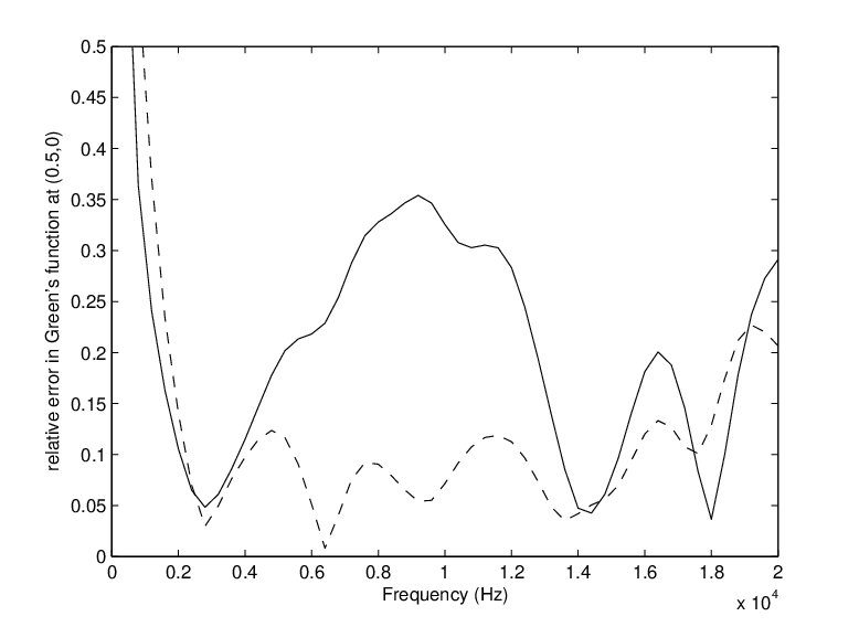
Numerical Green’s functions are calculated for zero and second order boundary conditions. The excitation is at point $(0,0)$ and the analytical solution in infinite space is given by formula (84). The Green’s functions are presented in figure 10 for a point at $(0.3,0)$ on the horizontal axis and in figure 11 for a point at $(0.3,0.3)$ along the diagonal. Good agreements between the two types of absorbing boundary conditions and the analytical solution can be observed. Both boundary conditions fail at low frequencies because the size of the domain is too small compared to the wavelength. Similarly the error for high frequencies are of same orders for both boundary conditions. For intermediate frequencies the error is lower for the second order boundary condition. This is more clearly seen in figure 12 where the relative error for the point $(0.3,0.3)$ is plotted versus the frequency.

The same results are presented in figure 13 for the point $(0.3,0.3)$ and a mesh density of $80\times 80$ elements. The solution is clearly much better at high frequencies meaning that the errors seen in figures 10 and 11 can be explained by elements too large for these frequencies and not by the quality of the boundary conditions. In figure 14 the domain is now $2m\times 2m$ with $80\times 80$ elements, so with elements of the same size as for figures 10 and 11. Results are plotted for the point $(0.3,0.3)$ . Now the improvement is clearly seen for low frequencies while there is no difference for high frequencies.

4.2 Two dimensional elastodynamics

The analytical solution in direction $e_{n}$ of the two dimensional elastodynamics case when submitted to a unit force at origin in direction $e_{m}$ , is given by

G_{nm}(r)=\frac{i}{4\mu}\left[A\delta_{nm}+B\frac{x_{n}x_{m}}{r^{2}}\right]

(106)

with:

	$\displaystyle A$	$\displaystyle=$	$\displaystyle H_{0}(K_{T}r)-\frac{1}{K_{T}r}\left[H_{1}(K_{T}r)-\beta H_{1}(K_{L}r)\right]$
	$\displaystyle B$	$\displaystyle=$	$\displaystyle-2A+\left[H_{0}(K_{T}r)+\beta^{2}H_{0}(K_{L}r)\right]$

where $H_{0}$ and $H_{1}$ are the Hankel functions of first type, of orders zero and one respectively. The wavenumbers are $K_{L}=\omega/c_{L}$ and $K_{T}=\omega/c_{T}$ for the longitudinal and transverse waves respectively. The velocities $c_{L}$ , $c_{T}$ and the ratio between them $\beta$ are given by,

\left\{\begin{array}[]{rcl}\beta&=&\displaystyle\frac{c_{T}}{c_{L}}\\ c_{L}^{2}&=&\displaystyle\frac{\lambda+2\mu}{\rho}\\ c_{T}^{2}&=&\displaystyle\frac{\mu}{\rho}\end{array}\right.\quad\mathrm{with}\quad\lambda=\frac{E\nu}{(1+\nu)(1-2\nu)}\quad\mathrm{and}\quad\mu=\frac{E}{2(1+\nu)}

(107)

In this example, the same global meshes as for the acoustic case are used. The boundary condition is computed from the square four nodes elements. The material is steel with $E=2.10^{11}Pa$ , $\nu=0.3$ and $\rho=7800kg/m^{3}$ and plane strain conditions are used in the computation. The sizes of the periodic cell can be $b=0.025m,\,0.0125m$ or $0.00625m$ .

In figure 15, numerical solutions are compared with analytical solutions for the point $(0.5,\,0)$ and $(0,\,0.5)$ for different sizes of the cell. The curves represent the real and imaginary parts of the first component of the displacement for an excitation at origin in direction 1. The same remarks as the previous examples can be made: $1)$ a denser mesh leads to lower errors over the high frequency band $[8.10^{3}Hz,\,20.10^{3}Hz]$ ; $2)$ for the low frequency band $[0,\,8.10^{3}Hz]$ , numerical results are different from the analytical solutions due to the finite size of the domain $(L=1m)$ .

In figure 16, the results for these two points are presented when the size of the domain is increased successively with $L=1m,\,2m$ and $4m$ . In this case, when the size of the cell is fixed to $b=0.025m$ , a larger domain leads to lower errors over the low frequency band $[0,\,8.10^{3}Hz]$ . The results are the same as previously in the high frequency band because in this domain the precision depends on the size of the elements and not on the size of the global domain. Some improvements are however seen for intermediate frequencies.

In figure 17 the error for boundary conditions of zero and second orders are plotted versus the frequency. The second order condition is much more accurate for intermediate frequencies as for the acoustic case.

5 Conclusion

In this paper, a method to determine absorbing boundary conditions for two dimensional periodic media has been presented. It works directly on the discretized equations. The boundary condition is first obtained as a global impedance relation and is then localized into boundary conditions of various orders. In two examples, good agreements were observed when compared with analytical solutions.

In any case, the proposed method is efficient because it requires only the discrete dynamic matrices which can be obtained by any standard finite element software. This method could be used for media with more complex behaviors than those presented in the precedent examples.

References

[1] C.A. Brebbia, S. Walker, Boundary elements techniques in engineering, Newnes-butterworths, London, England, 1980.
[2] S.L. Crouch, A.M. Starfield, Boundary element methods in solid mechanics, Unwin Hyman, London, England, 1990.
[3] R.D. Ciskowski, C.A. Brebbia, Boundary element methods in acoustics, Computational mechanics publications, Elsevier, Southampton, England, 1991.
[4] G. Chen, J. Zhou, Boundary element methods, Computational mathematics and applications, Academic press, London, 1992.
[5] M. Bonnet, Boundary integral equation methods for solids and fluids, Wiley, Chichester, England, 1995.
[6] A.H.D. Cheng, D.T. Cheng, Heritage and early history of the boundary element method, Engrg. Anal. Bound. Elem., 29 (2005) 268-302.
[7] D.E. Beskos, Boundary element methods in dynamic analysis: Part II (1986-1996), Applied mechanics reviews, 50 (1997) 149-197.
[8] J.B. Keller, D. Givoli, A finite element method for large domains, Comput. Methods Appl. Mech. Engrg., 76 (1989) 41-66.
[9] J.B. Keller, D. Givoli, Exact non reflecting boundary conditions, J. Comput. Physics, 82 (1989) 172-192.
[10] J.T. Hunt, M.R. Knittel, D. Barach, Finite element approach to acoustic radiation from elastic structures, J. Acoust. Soc. Amer., 55 (1974) 269-280.
[11] J.T. Hunt, M.R. Knittel, C.S. Nichols, D. Barach, Finite element approach to acoustic scattering from elastic structures, J. Acoust. Soc. Amer., 57 (1975) 287-299.
[12] I. Harari, T.J.R. Hughes, Finite element methods for the Helmholtz equation in an exterior domain: model problems, Comput. Methods Appl. Mech. Engrg., 87 (1991) 59-96.
[13] L.L. Thompson, R. Huan, Finite element formulation of exact non-reflecting boundary conditions for the time-dependent wave equation, Int. J. Numer. Methods Engrg., 45 (1999) 1607-1630.
[14] J.M. Galan, R. Abascal, Elastodynamic guided wave scattering in infinite plates, Int. J. Numer. Methods Engrg, 58 (2003) 1091-1118.
[15] P. Bettess, Infinite elements, Int. J. Numer. Methods Engrg., 11 (1977) 53-64.
[16] P. Bettess, More on infinite elements, Int. J. Numer. Methods Engrg., 15 (1980) 1613-1626.
[17] P. Bettess, C. Emson, T.C. Chiam, Numerical Methods in Coupled Systems, Edited by R.W. Lewis, P. Bettes and E. Hinton, A new mapped infinite element for exterior wave problems, chap 17, (1984) 489-504.
[18] P. Bettess, Infinite elements, Penshaw Press, 1992.
[19] R.J. Astley, Infinite elements for wave problems: a review of current formulations and an assessment of accuracy, Int. J. Numer. Methods Engrg., 49 (2000) 951-976.
[20] D.S. Burnett, A three-dimensional acoustic infinite element based on a prolate spheroidal multipole expansion, J. Acoust. Soc. Am., 96 (1994) 2798-2816.
[21] K. Gerdes, A review of infinite element methods for exterior Helmholtz problems, J. Comput. Acoustics, 8 (2000) 43-62.
[22] J.P. Bérenger, A perfectly matched layer for the absorption of electromagnetic waves, J. Comput. Physics, 114 (1994) 185-200.
[23] J.P. Bérenger, Three-dimensional perfectly matched layer for the absorption of electromagnetic waves, J. Comput. Physics, 127 (1996) 363-379.
[24] F. Colino, P.B. Monk, Optimizing the perfectly matched layer, Comput. Methods Appl. Mech. Engrg., 164 (1998) 157-171.
[25] S. Asvadurov, V. Druskin, M.N. Guddati, L. Knizhnerman, On optimal finite-difference approximation of PLM, SIAM J. Numer. Anal., 41 (1) (2003) 287-305
[26] B. Engquist, A. Majda, Absorbing boundary conditions for the numerical simulation of waves, Mathematics of computation, 31 (1977) 629-651.
[27] T. Strouboulis, R. Hidajat, I. Babuska, The generalized finite element method for Helmholtz equation. Part II: Effect of choice of handbook functions, error due to absorbing boundary conditions and its assessment, Comput. Methods Appl. Mech. Engrg., 197 (2008) 364-380.
[28] P.M. Pinsky, L.L. Thompson, N.N. Abboud, Local high-order radiation boundary conditions for the two-dimensional time-dependent structural acoustics problem, J. Acoust. Soc. Am., 91 (1992) 1320-1335.
[29] M.N. Guddati, K.W. Lim, Continued fraction absorbing boundary conditions for convex polygonal domains, Int. J. Numer. Methods Engrg, 66 (2006) 949-977.
[30] E. Heikkola, T. Rossi, J. Toivanen, Fast direct solution of the Helmholtz equation with a perfectly matched layer or an absorbing boundary condition, Int. J. Numer. Methods Engrg, 57 (2003) 2007-2025.
[31] D. Givoli, High-order local non-reflecting boundary conditions: a review, Wave Motion, 39 (2004) 319-326.
[32] S. Krenk, P.H. Kirkegaard, Local tensor radiation conditions for elastic waves, J. Sound Vib., 247 (2001) 875-896.
[33] O. Guasch, R. Codina, An algebraic subgrid scale finite element method for the convected Helmholtz equation in two dimensions with applications in aeroacoustics, Comput. Methods Appl. Mech. Engrg., 196 (2007) 4672-4689.
[34] M.A. Storti, N.M. Nigro, R.R. Paz, L.D. Dalcin, Dynamic boundary conditions in computational fluid dynamics, Comput. Methods Appl. Mech. Engrg., 197 (2008) 1219-1232.
[35] D. Givoli, Non-reflecting boundary conditions: a review, J. Comput. Physics, 94 (1991) 1-29.
[36] E. Mesquita, R. Pavanello, Numerical methods for the dynamics of unbounded domains, Computational & applied mathematics, 24 (2005) 1-26.
[37] I. Harari, A survey of finite element methods for time-harmonic acoustics, Comput. Methods Appl. Mech. Engrg., 195 (2006) 1594-1607.
[38] L.L. Thompson, A review of finite element methods for time-harmonic acoustics, J. Acoust. Soc. Am., 119 (2006) 1315-1330.
[39] B.R. Mace, D. Duhamel, M.J. Brennan, L. Hinke, Finite element prediction of wave motion in structural waveguides, J. Acous. Soc. Amer., 117 (2005) 2835-2843.
[40] D. Duhamel, B.R. Mace, M.J. Brennan, Finite element analysis of the vibrations of waveguides and periodic structures, J. Sound Vib., 294 (2006) 205-220.
[41] D. Duhamel, Finite element computation of Green’s functions, Engrg. Anal. Bound. Elem., 31 (2007) 919-930.

Refer to caption — Figure 1: Computational domain