Microlensing Evidence That A Type 1 Quasar Is Viewed Face On
Abstract
Using a microlensing analysis of 11-years of OGLE V-band photometry of the four image gravitational lens Q2237+0305, we measure the inclination of the accretion disk to be at 68% confidence. Very edge on () solutions are ruled out at 95% confidence. We measure the V-band radius of the accretion disk, defined by the radius where the temperature matches the monitoring band photon emission, to be assuming a simple thin disk model and including the uncertainties in its inclination. The projected radiating area of the disk remains too large to be consistent with the observed flux for a thin disk temperature profile. There is no strong correlation between the direction of motion (peculiar velocity) of the lens galaxy and the orientation of the disk.
Subject headings
gravitational lensing — methods: numerical — quasars: general — quasars: individual (Q2237+0305) —I. Introduction
In the AGN unification model [4, 38, e.g.], orientation differences among intrinsically similar objects are thought to account for many of the different observational properties of AGN. In particular, a dusty “torus” may frequently obscure the central engine from direct observation when viewed edge-on. The bright, Type 1 broad line quasars are thought to be viewed mostly face-on, so that the accretion disk is not obscured by material in the equatorial plane, and Type 2 narrow line quasars are viewed closer to edge-on through the obscuring material. Thus, if we could resolve the disk of a Type 1 quasar, we would expect it to be closer to face-on than edge-on. Unfortunately, familiar methods cannot resolve accretion disks, so we have only indirect measures of AGN disk orientation. For example, the projected axes of radio jets [7] and ionization cones [13] both support this picture. There are, however, no actual measurements of disk orientation.
While quasar accretion disks are too small to be resolved by direct imaging, gravitational microlensing provides a natural telescope to study the structure of quasar accretion disks and the properties of cosmologically distant lens galaxies where we see multiple images of background quasars [41, see]. In addition to the mean potential of the lens galaxy, each image is also magnified by the microlensing effects of the nearby stars. Since the observer, the lens galaxy and its stars, and the quasar are all moving, microlensing is observed as uncorrelated time variability in each of the quasar images. The amplitudes of these variations depend on the structure of the accretion disk and the properties of the lens galaxy.
Quasar microlensing is most sensitive to the projected area of the accretion disk relative to the source plane Einstein radius,
| (1) | |||||
where is the gravitational constant, is the speed of light, is the mean stellar mass of the stars, , and are the angular diameter distances between the lens-source, observer-lens, and observer-source respectively, and we have used the lens and source redshifts for Q2237+0305 [, 20, Q2237 hereafter]. The smaller the accretion disk, the higher the variability amplitude from microlensing. In general, the emission profile is difficult to determine, as models having similar half light radii show similar microlensing variability [28]. There has been little examination of other structural parameters of disks, except for Congdon et al. [9], who demonstrated in simulations that the microlensing signal is sensitive to the ellipticity and orientation of the accretion disk. If detectable in practice, measuring the apparent ellipticities of accretion disks provides an important test of AGN unification models and opens the possibility of examining the complex effects of relativity on the apparent surface brightness of the disk [19, e.g.].
Measurements of quasar disk sizes using microlensing are now common. Recent efforts have studied individual sizes [26, e.g.], the relationships between size and wavelength [3, 5, 12, 31, 14, 29], size and black hole mass [25], and the sizes of thermal and non-thermal emission regions [33, 27, 8, 10]. All these studies used circular accretion disks and static magnification patterns that neglect the random motion of stars in the lens galaxy.

Determining the shape and orientation of a disk depends on the correlations between the anisotropic structure of the disk and the anisotropic structure in the magnification patterns created by the shear (tidal gravity) local to each image (see Figure 1, Congdon et al. 9). Existing microlensing studies cannot safely explore these issues because they neglect the motions of the stars in the lens galaxy and use “static” magnification patterns. Since the stellar velocity dispersions of lens galaxies are comparable to the peculiar velocities of galaxies, the patterns change on the same time scale as the source traverses them. Ignoring these stellar motions will overestimate the coherence of the magnification patterns [43, 22, see] and likely render estimates of disk shapes unrealistic. With a few exceptions that do not focus on disk structure (see Paper I and Wyithe et al. [42]), analyses of microlensing data have used static magnification patterns because of the computational challenges. In Paper I [32], we solved these computational problems and examined the peculiar velocity of the lens galaxy of Q2237 and the mean mass of its stars. In this paper, we measure the size, inclination, and position angle of the accretion disk in Q2237. In §II we describe the data set used for our microlensing analysis, our disk model, and outline our overall approach. Our results are presented in §III, and a discussion follows in §IV.
II. Data and Methods
We analyze the nearly 11 years of Optical Gravitational Lensing Experiment (OGLE) V-band photometric monitoring data for Q2237 [37]. To speed our analysis and as a cross check on the results, we divided the data into two separate light curves. The first light curve (LC1 hereafter) ranges from JD 2,450,663 to JD 2,452,621 and consists of 100 epochs. The second light curve (LC2 hereafter) has 230 epochs from JD 2,452,763 to JD 2,454,602. Each light curve covers just over 5 years. We broaden the OGLE uncertainties by our estimate of the systematic uncertainties in the photometry of 0.02, 0.03, 0.04, and 0.05 magnitudes in quadrature [32].
We analyze these light curves using the Bayesian Monte Carlo method of Kochanek [21], expanded to include motions of stars as detailed in Paper I. For each epoch of the light curve we generate a magnification pattern including the random motion of the stars. We used fixed mean masses of and , and a mass function of with a dynamic range based on Gould [17]. In Paper I we find that the best fit to the data is for . The stars are assigned a random velocity in each coordinate from a Gaussian distribution with based on the observed velocity dispersion (van de Ven, G. 2009, personal communication, Trott et al. [36]). The orbit of Earth (parallax effect) and the rotation of the lens galaxy are both included in the simulation. We convolve the patterns with the disk models described in §II. We draw the bulk velocities of the observer, lens galaxy, and source from a Gaussian of dispersion on the lens plane in each coordinate. We later reweight the results to a more compact velocity prior based on the projection of the CMB dipole velocity [18] onto the lens plane, which is small , and the (1D) peculiar velocity dispersions of the lens and source of and [35, estimated from], respectively. Because of the low lens redshift and the small projected dipole, the peculiar velocity of the lens is by far the most important factor (see Paper I). We then randomly draw light curves for each image and fit them to the data. Bayes theorem is used to combine the goodness of fit for the trials as measured by a statistic, into probability distributions for each variable of interest. These procedures are described in detail in Kochanek [21] and Paper I.
II.1. Accretion Disk Model
We employ a generic thin disk model for which the surface temperature scales as with radius R [34]. The microlensing signal is primarily sensitive to the half-light radius of the disk [28], which controls the effective smoothing area of the disk, and, to date, studies have been unable to distinguish differing radial profiles [21, e.g.]. A more realistic disk model would include a central hole whose size depends on the last stable orbit and general relativistic effects modify the underlying intensity profiles [19, e.g.]. We have not presently pursued these features because they add many model parameters, and because it is unclear whether the temperature profile of the thin disk model is correct. In particular, microlensing studies suggest the need for a flatter temperature profile [33, 25, 31, 12, e.g.] in order to reconcile the microlensing sizes with the observed optical fluxes. Such changes in the temperature profile have also been suggested to explain the deviations of the observed spectral slope from the thin disk emission (see the reviews by [24] and [6]).
Thus, we assume that the face-on () surface brightness of the disk is
| (2) |
where
| (3) | |||||
corresponds to the radius where the disk temperature equals the photon energy, , is the black hole mass, is the accretion rate, is the luminosity relative to Eddington luminosity, and is the radiative efficiency of the accretion disk. The half light radius of the disk is . We now simply treat the disk as an infinitely thin disk viewed at inclination angles , selected from a uniform distribution in , and (face-on). We include no relationship between the surface brightness and the viewing angle other than this simple projection effect in this first exploration of the problem. For full relativistic disk models, there are many complexities such as Doppler shifts, redshifts, and bending of ray trajectories [1, e.g.], but the bulk of the optical flux comes from relatively large radii, for , where these effects are less important. Here we use Morgan et al. [25]’s estimated black hole mass of found by applying the virial relation of Vestergaard & Peterson [40] to the C IV line width measurement from Yee & De Robertis [45]. Since the orientation of the projected disk relative to the magnification patterns also affects the results, we considered 18 major axis position angles from to in steps of , where the remaining angles are covered by the reflection symmetry of the disk model. We parametrized the size of the disk by the projected area, , as this is likely to have less correlation with the inclination angle because it keeps the projected area of the disk constant.
We must also worry about whether all the observed emission arises directly from the accretion disk. The light curves can be contaminated by broad line emission on much larger scales or some of the emission from the disk can be scattered on larger scales [10, 27, 25, see]. At V-band, the contamination from broad line emission, mainly Fe pseudo-continuum emission and C III , contributes of order of the flux in the spectral models of Eigenbrod et al. [11]. To examine the effect of this dilution we ran models with , , and contamination by emission on large, un-microlensed scales for the case. Adding an unmicrolensed contamination fraction, , in the V-band also decreases the flux size estimate by unless the contamination is due to scattering of the disk emission on large scales [25, see the discussion in].
III. Results
We estimate the projected area of the accretion disk , the deprojected radius , the disk inclination , and the major axis position angle. We also do a limited set of tests with different amounts of unmicrolensed flux that may influence our analysis. We quote the results from the combined analysis of LC1 and LC2, but also show the results from the independent analyses of LC1 and LC2. Since the results are always mutually consistent, we only report quantitative results for the combined analysis.
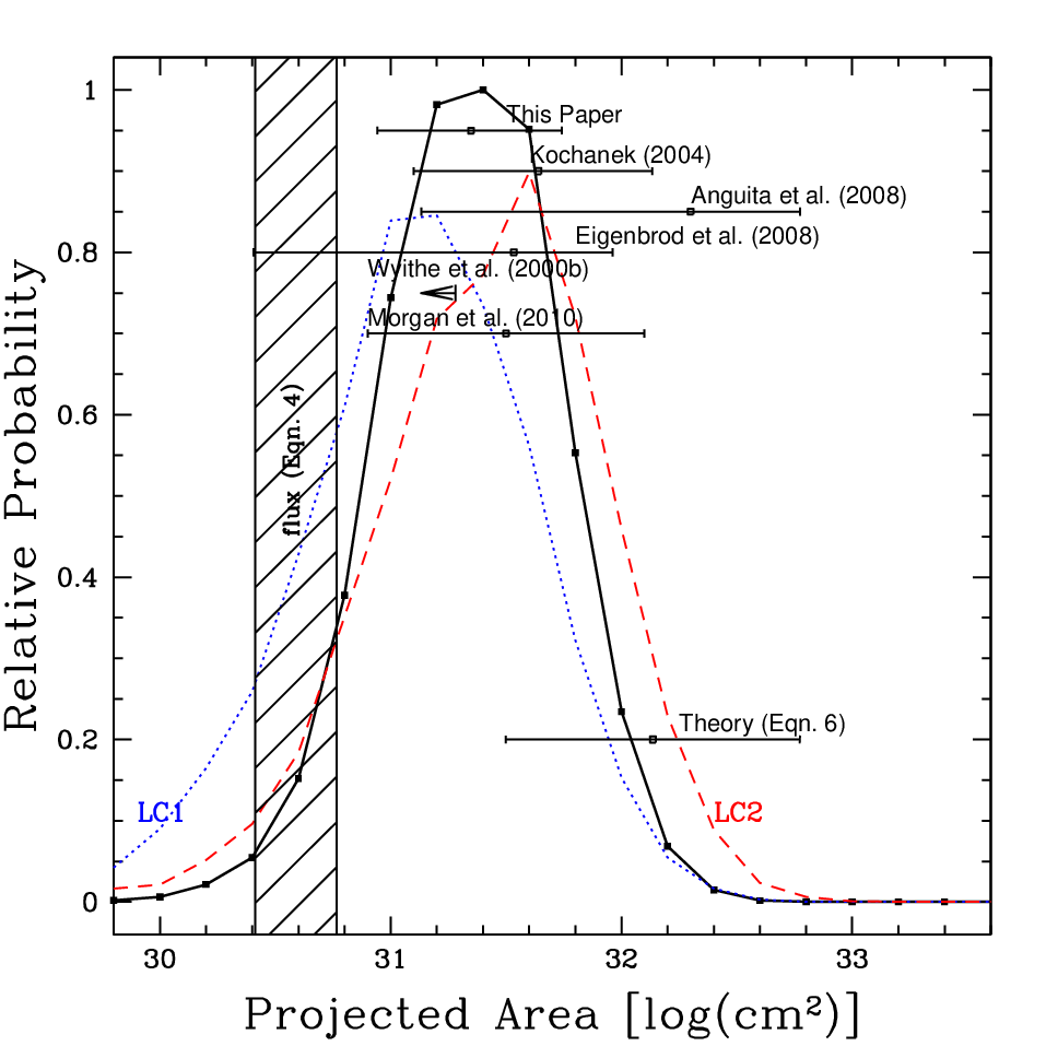
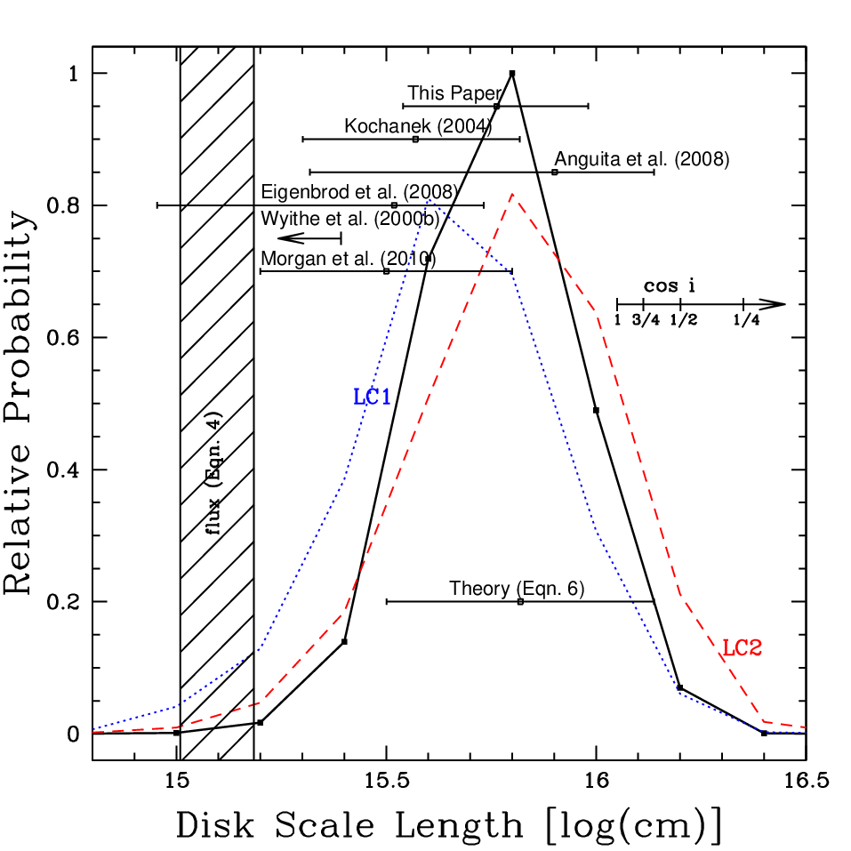
We find (Figure 2) the projected V-band area of the quasar defined by to be () at 68% (95%) confidence with a median of , where the size scale is defined by Equation 3. After de-projecting the area based on each trial’s inclination, we find that the V-band radius of the accretion disk is () at 68% (95%) confidence with a median value of (Figure 3). This is consistent with our earlier results in Kochanek [21] and Morgan et al. [25], of and using the same method without dynamic patterns, a smaller velocity prior, and shorter light curves. Other analyses by Wyithe et al. [44], Yonehara [46], Vakulik et al. [39], Anguita et al. [3], and Eigenbrod et al. [12] have found generally consistent results of (at 99% confidence), , , , and (see Figure 3), but using less data and with far stronger systematic assumptions. These estimates are all for and should scale as . If we compare projected areas (Figure 2), then the comparisons are (to 1st order) independent of the inclination angle, while if we compare disk scale lengths, there will be an inclination angle dependence. While generally consistent with our results, our calculations use more data and are considerably more realistic, making it difficult to evaluate differences, especially the uncertainties.
We can compare our measurement to those predicted by the observed fluxes or thin disk theory. If we assume only the temperature profile of a thin disk model [34], where we can ignore the inner disk edge for these wavelengths, then the observed flux constrains the disk size by matching the integrated flux from a disk with the emission profile of Equation 3 to the observed flux. We estimate that the magnification corrected I-band flux is mag, and this corresponds to a disk radius of
| (4) | |||||
where is the angular diameter distance to the quasar relative to the Hubble radius, [25, see]. This gives . Assuming our best fit inclination, , .
Agol et al. [2] estimate that the bolometric luminosity of the quasar is ergs s-1, which corresponds to a Eddington factor of
| (5) |
that is typical of luminous quasars [23]. If we use this to replace the factor in Eqn. 3, the size estimate becomes
| (6) |
which now depends relatively weakly on the black hole mass. The uncertainties in these estimates are logarithmic, corresponding to and dex respectively for Eqns. 3 and 6 if the masses, Eddington factors, luminosities and efficiencies are viewed as being uncertain by a factor of . We find that the disk is large compared to the estimate based on the observed flux, although this is modestly reduced by the inclination, and small compared to a thin disk radiating close to Eddington with efficiency. This is a discrepancy common to all microlensing estimates at present [33, 25, see].
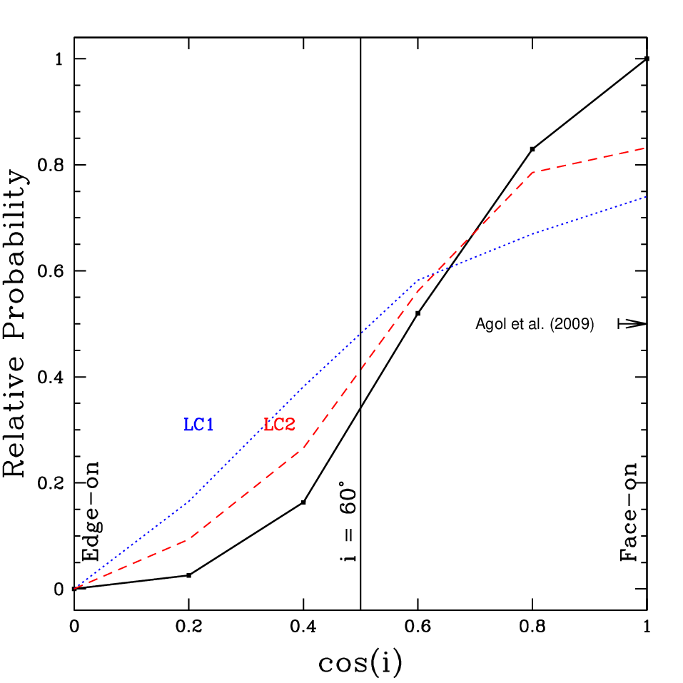
Where these size estimates are incremental improvements over earlier results from using additional data and an improved physical model, our results for the inclination and orientation of the disk are entirely new. The preferred inclination is at 68% confidence where is face-on (Figure 4). Such a relatively face-on inclination is consistent with the expectations of the AGN unification model. We can compare this to Agol et al. [2]’s model for the mid-infrared spectral energy distribution of Q2237 using the dust torus models of Fritz et al. [15]. While Agol et al. [2] do not trust the quantitative results, their preferred viewing angles (, Figure 4) are consistent with our inferences for the inclination angle of the disk.
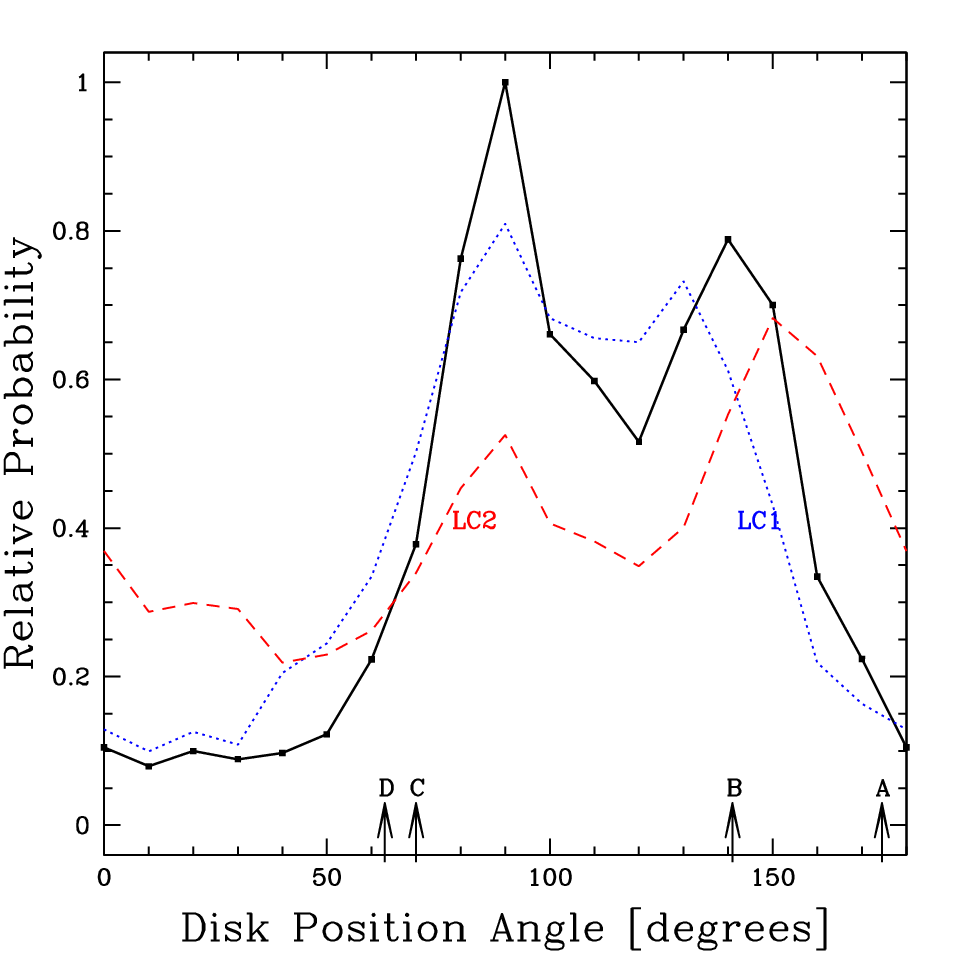
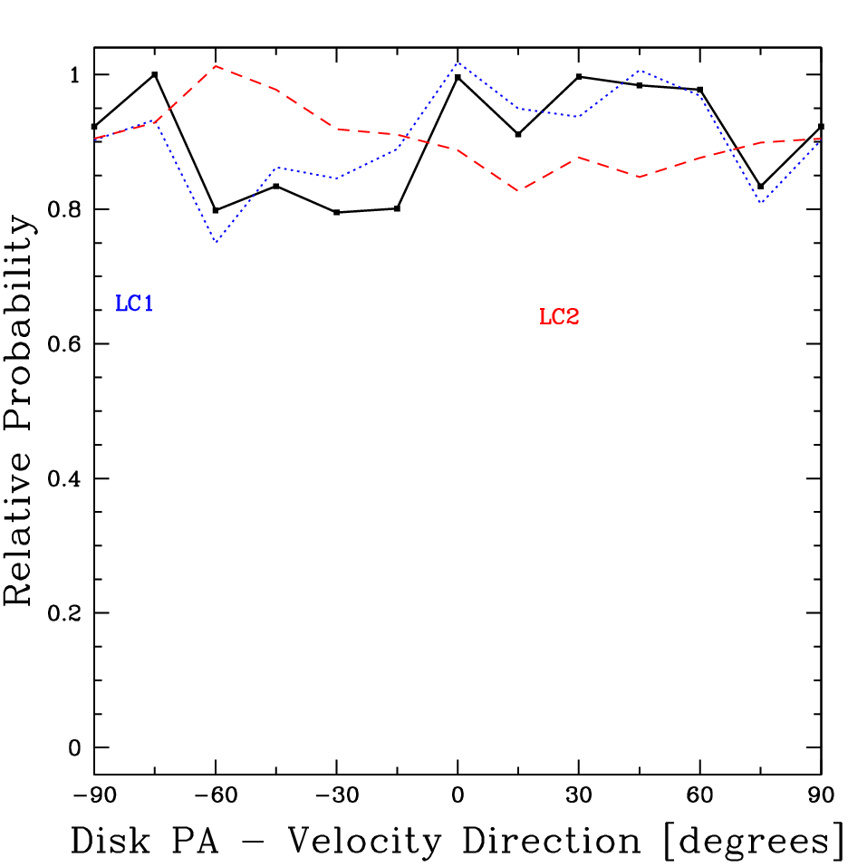
Figure 5 shows our estimate of the position angle (PA) of the major axis of the disk, and Figure 1 shows the 68% confidence range of this PA for comparison to the anisotropies in the magnification patterns. We find consistent estimates of this position angle from both LC1 and LC2 (Figure 5). The preferred orientation is for the major axis to be roughly parallel to the shear in image B, but perpendicular to it in images C and D. Congdon et al. [9] found that microlensing variability is enhanced when the major axis is aligned with the shear, so our estimated alignment helps to explain the higher variability of images A and B, and the lower variability of D, but not the variability of image C. For this lens there are no other observations to which we can compare the orientation. However, if we had observations of the quasar host galaxy, we could compare the PA of the galaxy to that of the disk as a check on the relative orientations of the angular momentum vectors of the accretion disk and the galaxy. For example, Yoo et al. [47], Yoo et al. [48] used images of lensed quasar hosts to constrain the host axis ratio and position angle in 4 lensed quasars (to roughly ). While both the peculiar velocity direction of the lens and the disk position angle are constrained, we find no strong constraints on the disk orientation relative to the direction of motion (Figure 6). The convolved uncertainties in the two quantities are too large.
Luminosity that originates outside the accretion disk proper is a concern for size estimates because contamination by emission on large scales dilutes the microlensing signal and leads us to overestimate the projected area of the disk [10, 27, see]. To examine this effect, we did a set of trials with where 0%, 20%, and 40% of the source light was not microlensed. The spectral analysis by Eigenbrod et al. [11] suggests that the level of contamination is 20%. The 0% and 20% cases fit equally well, while the 40% case had a relative probability 38% lower. As the dilution is increased from 0%, more face-on disks are preferred, with and (68% confidence) for 0%, 20%, and 40% dilution. Adding unmicrolensed light affects the disk size both through the general dilution and the shift towards more face-on orientations. The de-projected radius is smaller by if the contamination is increased to 20% (40%) from 0%. These corrections are not large compared to our statistical uncertainties of order 70%, but they are an important physical consideration.
IV. Discussion
By including random stellar motions in our microlensing analysis of Q2237 we find evidence that the accretion disk of Q2237 is viewed face-on with . This lends support to the popular AGN unification model where we expect Type 1 quasars like Q2237 to be viewed nearly face-on. Including 20% contamination from broad line emission on larger spatial scales [11, estimated from spectra] results in a stronger case for face-on solutions. Modeling stellar motions and the inclination and position angle parameters further reduces the systematic uncertainties of our measurements of the disk radius compared to earlier studies by including a broader range of physical uncertainties. As we found in Paper I for the lens velocity and mean stellar mass, the results of the separate analyses of LC1 and LC2, the first and second temporal halves of the OGLE light curves, produce consistent results for every parameter we considered. While we have used a relatively simple model for the accretion disk, these results demonstrate that disk shapes can be measured with quasar microlensing, as suggested by Congdon et al. [9]. As data sets and computing power improve, it will be natural to try fitting more subtle disk features such as the asymmetries from relativistic effects using relativistic models such as Hubeny et al. [19].
The exceptionally long OGLE light curve and the fast microlensing timescales of Q2337 made it a natural first choice for including the random stellar motions and studying the shape of the disk. Our expanded method is similar in computational cost to our previous efforts with static patterns, so there is no reason not to use it generally. The stellar motions clearly aid in reducing uncertainties in the mean mass (see Paper I) and allow us to correctly make inclination corrections. It can also easily be extended to take advantage of multi-wavelength data to try to constrain the temperature profile. However, as in earlier microlensing studies [33, 25, 10], we cannot reconcile the basic temperature profile of a thin disk, the microlensing size estimate, and the observed optical flux. A disk with a temperature profile normalized by the microlensing size estimate should be brighter than observed. This can be solved by altering the temperature profile [31, 25, see]. For example, reducing the slope from to would increase the flux size by a factor of relative to the half light radius. This would be mildly inconsistent () with the slope estimate of by Eigenbrod et al. [12]. However such changes also call into question the basic structure of the thin disk model. The other simple possibility is to reduce the emissivity of the disk to be well below that of a blackbody (by the ratio of the flux/microlensing sizes squared), but this seems less physically plausible than change in the temperature structure.
References
- [1] Agol, E. 1997, Ph.D. Thesis,
- [2] Agol, E., Gogarten, S. M., Gorjian, V., & Kimball, A. 2009, ApJ, 697, 1010
- [3] Anguita, T., Schmidt, R. W., Turner, E. L., Wambsganss, J., Webster, R. L., Loomis, K. A., Long, D., & McMillan, R. 2008, A&A, 480, 327
- [4] Antonucci, R. 1993, ARA&A, 31, 473
- [5] Bate, N. F., Floyd, D. J. E., Webster, R. L., & Wyithe, J. S. B. 2008, MNRAS, 391, 1955
- [6] Blaes, O.M., 2004, in Les Houches Summer School LXXVIII (Springer: Berlin) 137
- [7] Blandford, R. D., & Konigl, A. 1979, ApJ, 232, 34
- [8] Chartas, G., Kochanek, C. S., Dai, X., Poindexter, S., & Garmire, G. 2009, ApJ, 693, 174
- [9] Congdon, A. B., Keeton, C. R., & Osmer, S. J. 2007, MNRAS, 376, 263
- [10] Dai, X., Kochanek, C. S., Chartas, G., Kozlowski, S., Morgan, C. W., Garmire, G., & Agol, E. 2009, arXiv:0906.4342
- [11] Eigenbrod, A., Courbin, F., Sluse, D., Meylan, G., & Agol, E. 2008a, A&A, 480, 647
- [12] Eigenbrod, A., Courbin, F., Meylan, G., Agol, E., Anguita, T., Schmidt, R. W., & Wambsganss, J. 2008, A&A, 490, 933
- [13] Elvis, M. 2000, ApJ, 545, 63
- [14] Floyd, D. J. E., Bate, N. F., & Webster, R. L. 2009, arXiv:0905.2651
- [15] Fritz, J., Franceschini, A., & Hatziminaoglou, E. 2006, MNRAS, 366, 767
- [16] Gil-Merino, R., Wambsganss, J., Goicoechea, L. J., & Lewis, G. F. 2005, A&A, 432, 83
- [17] Gould, A. 2000, ApJ, 535, 928
- [18] Hinshaw, G., et al. 2009, ApJS, 180, 225
- [19] Hubeny, I., Blaes, O., Krolik, J. H., & Agol, E. 2001, ApJ, 559, 680
- [20] Huchra, J., Gorenstein, M., Kent, S., Shapiro, I., Smith, G., Horine, E., & Perley, R. 1985, AJ, 90, 691
- [21] Kochanek, C. S., 2004, ApJ, 605, 58
- [22] Kochanek, C. S., Dai, X., Morgan, C., Morgan, N., Poindexter, S. & Chartas, G., 2007, in Statistical Challenges in Modern Astronomy IV in Statistical Challenges in Modern Astronomy IV G. J. Babu and E. D. Feigelson, eds., (Astron. Soc. Pacific: San Francisco), [astro-ph/0609112]
- [23] Kollmeier, J.A., et al. 2006, ApJ, 648, 128
- [24] Koratkar, A & Blaes, O. 1999, PASP, 111, 1
- [25] Morgan, C., Kochanek, C.S., Morgan, N.D., Falco, E.E., 2010, ArXiv e-prints, 707, arXiv:0707.0305, in prep.
- [26] Morgan, C. W., Eyler, M. E., Kochanek, C. S., Morgan, N. D., Falco, E. E., Vuissoz, C., Courbin, F., & Meylan, G. 2008, ApJ, 676, 80
- [27] Morgan, C. W., Kochanek, C. S., Dai, X., Morgan, N. D., & Falco, E. E. 2008, ApJ, 689, 755
- [28] Mortonson, M. J., Schechter, P. L., & Wambsganss, J. 2005, ApJ, 628, 594
- [29] Mosquera, A. M., Muñoz, J. A., & Mediavilla, E. 2009, ApJ, 691, 1292
- [30] Peng, C. Y., Impey, C. D., Rix, H.-W., Kochanek, C. S., Keeton, C. R., Falco, E. E., Lehár, J., & McLeod, B. A. 2006, ApJ, 649, 616
- [31] Poindexter, S., Morgan, N., & Kochanek, C. S. 2008, ApJ, 673, 34
- [32] Poindexter, S. & Kochanek, C. S. 2009, arXiv:0910.3213
- [33] Pooley, D., Blackburne, J. A., Rappaport, S., & Schechter, P. L. 2007, ApJ, 661, 19
- [34] Shakura, N.I. & Sunyaev, R.A., 1973, A&A, 24, 337
- [35] Tinker, J. L. & Wetzel, A. R., Zehavi, I., 2009, in prep.
- [36] Trott, C. M., Treu, T., Koopmans, L. V. E., & Webster, R. L. 2008, arXiv:0812.0748
- [37] Udalski, A., et al. 2006, Acta Astronomica, 56, 293
- [38] Urry, C. M., & Padovani, P. 1995, PASP, 107, 803
- [39] Vakulik, V. G., Schild, R. E., Smirnov, G. V., Dudinov, V. N., & Tsvetkova, V. S. 2007, MNRAS, 382, 819
- [40] Vestergaard, M. & Peterson, B.M. 2006, ApJ, 641, 689
- [41] Wambsganss, J, 2006, in Gravitational Lensing: Strong Weak and Micro, Saas-Fee Advanced Course 33, G. Meylan, P. North, P. Jetzer, eds., (Springer: Berlin) 453, [astro-ph/0604278]
- [42] Wyithe, J. S. B., Webster, R. L., & Turner, E. L. 1999, MNRAS, 309, 261
- [43] Wyithe, J. S. B., Webster, R. L., & Turner, E. L. 2000, MNRAS, 315, 51
- [44] Wyithe, J. S. B., Webster, R. L., & Turner, E. L. 2000, MNRAS, 318, 762
- [45] Yee, H.K.C. & De Robertis, M.M. 1991, ApJ, 381, 386
- [46] Yonehara, A. 2001, ApJ, 548, L127
- [47] Yoo, J., Kochanek, C. S., Falco, E. E., & McLeod, B. A. 2005, ApJ, 626, 51
- [48] Yoo, J., Kochanek, C. S., Falco, E. E., & McLeod, B. A. 2006, ApJ, 642, 22