Multiple Scattering Casimir Force Calculations: Layered and Corrugated Materials, Wedges, and Casimir-Polder Forces

Kimball A. Milton Email: milton@nhn.ou.edu Affiliation: Oklahoma Center for High Energy Physics, and H. L. Dodge Department of Physics and Astronomy, University of Oklahoma, Norman, OK 73019-2061, USA Prachi Parashar Email: prachi@nhn.ou.edu Affiliation: Oklahoma Center for High Energy Physics, and H. L. Dodge Department of Physics and Astronomy, University of Oklahoma, Norman, OK 73019-2061, USA Jef Wagner Email: wagner@nhn.ou.edu Affiliation: Oklahoma Center for High Energy Physics, and H. L. Dodge Department of Physics and Astronomy, University of Oklahoma, Norman, OK 73019-2061, USA I. Cavero-Peláez Email: cavero@nhn.ou.edu Affiliation: Theoretical Physics Department, Zaragoza University, Zaragoza, Spain

August 24, 2026

Abstract

Various applications of the multiple scattering technique to calculating Casimir energy are described. These include the interaction between dilute bodies of various sizes and shapes, temperature dependence, interactions with multilayered and corrugated bodies, and new examples of exactly solvable separable bodies.

pacs

03.70.+k, 03.65.Nk, 11.80.La, 42.50.Lc

I Introduction

For many years, calculation of Casimir or quantum vacuum energies were confined to systems of very high symmetry, such as parallel plates [1, 2]. Self-energies of spheres [3] and cylinders [4] were also calculated. To calculate the force between curved surfaces, such as that in the experimentally realizable spherical lens above a plate, resort had to be made to the “proximity force approximation” [5], which, while exact for zero separation, was subject to unknown corrections for finite distances between the surfaces.

That situation has radically changed. The “multiple scattering” technique, not merely increase in computing power, has been responsible for much of the improvement. The method, related to the Krein trace formula [6], was used early on to construct the Lifshitz formula for the quantum fluctuation force between dielectric plates [7]. It was the basis of the classic work by Balian and Duplantier [8]. But recently it was realized by many people that it could be applied to practical calculations of Casimir forces between bodies of essentially arbitrary shape and orientation [9, 10, 11, 12, 13, 14]. For more complete references and background, see Refs. [15, 16]. Complementary developments by Gies and collaborators on the worldline method [17, 18, 19, 20], and direct numerical methods [21, 22, 23] should also be cited.

In this paper we summarize the work of the Oklahoma group in applying the multiple scattering technique to a variety of problems. The hope is that results will be forthcoming that would be of use in the design of nanotechnology. We will merely summarize some representative results here; for more complete details and further applications the reader is referred to the original previous and forthcoming papers.

II Multiple Scattering Technique

For simplicity, we first restrict attention to the quantum vacuum forces arising from a massless scalar field. The multiple scattering approach starts from the well-known formula for the vacuum energy or Casimir energy

E=\frac{i}{2\tau}\mbox{Tr}\ln G\to\frac{i}{2\tau}\mbox{Tr}\ln GG_{0}^{-1},

(1)

where $\tau$ is the “infinite” time that the configuration exists, and $G$ ( $G_{0}$ ) is the Green’s function, which satisfies the differential equation

(-\partial^{2}+V)G=1,\quad-\partial^{2}G_{0}=1,

(2)

in terms of the background potential $V$ .

Now we define the $T$ -matrix,

T=S-1=V(1+G_{0}V)^{-1}.

(3)

If the potential has two disjoint parts, $V=V_{1}+V_{2}$ , it is easy to derive

T=(V_{1}+V_{2})(1-G_{0}T_{1})(1-G_{0}T_{1}G_{0}T_{2})^{-1}(1-G_{0}T_{2}),

(4)

T_{i}=V_{i}(1+G_{0}V_{i})^{-1},\quad i=1,2.

(5)

Thus, we can write the general expression for the interaction between the two bodies (potentials):

E_{12}=-\frac{i}{2\tau}\mbox{Tr}\ln(1-G_{0}T_{1}G_{0}T_{2})=-\frac{i}{2\tau}\mbox{Tr}\ln(1-V_{1}G_{1}V_{2}G_{2}),

(6)

where $G_{i}=(1+G_{0}V_{i})^{-1}G_{0},\quad i=1,2$ .

II.1 Exact Results for Weak Coupling

In weak coupling, where the potentials are very small, it is possible to derive the exact (scalar) interaction between two potentials [24], either in 2- or 3-dimensions:

	$2D:\quad\frac{E}{L_{z}}=-\frac{1}{32\pi^{3}}\int(d\mathbf{r_{\perp}})(d\mathbf{r_{\perp}^{\prime}})\frac{V_{1}(\mathbf{r_{\perp}})V_{2}(\mathbf{r_{\perp}^{\prime}})}{\|\mathbf{r-r^{\prime}}\|^{2}},$	(7a)
where $L_{z}$ is the “infinite” length in the translationally-invariant direction, and
	$3D:\quad E=-\frac{1}{64\pi^{3}}\int(d\mathbf{r})(d\mathbf{r^{\prime}})\frac{V_{1}(\mathbf{r})V_{2}(\mathbf{r^{\prime}})}{\|\mathbf{r-r^{\prime}}\|^{3}}.$	(7b)

Consider two plates (ribbons) of finite width $L$ , offset by an amount $b$ , separated by a distance $a$ , as shown in Fig. 1,


$\displaystyle V_{1}(\mathbf{r_{\perp}})$	$\displaystyle=$	$\displaystyle\lambda_{1}\delta(y)\theta(x)\theta(L-x),$	(8a)
$\displaystyle V_{2}(\mathbf{r_{\perp}^{\prime}})$	$\displaystyle=$	$\displaystyle\lambda_{2}\delta(y^{\prime}-a)\theta(x^{\prime}-b)\theta(L+b-x^{\prime}),$	(8b)

Refer to caption — Figure 1: Two ribbons of finite width, offset from each other. The ribbons have infinite extent out of the page.

Equation (7a) gives an explicit result for the energy of interaction between the plates:

\frac{E}{L_{z}}=-\frac{\lambda_{1}\lambda_{2}}{32\pi^{3}}\left[-2g(b/a)+g((L-b)/a)+g((L+b)/a)\right],

(9)

where

g(x)=x\tan^{-1}x-\frac{1}{2}\ln(1+x^{2})=-\mbox{Re}(1+ix)\ln(1+ix).

(10)

We can consider arbitrary lengths and orientations, in 3 dimensions, for the plates [24].

For example, we can consider tilted plates, as shown in Fig. 2.

Explicit interaction energies can be given in terms of $\mbox{Ti}_{2}$ , the inverse tangent integral. For fixed distance $D$ between the center of masses of the plates, and for $L_{1}\to L$ , $L_{2}\to\infty$ , $d\to-\infty$ (that is, the upper plate is completely above the much wider lower plate), and if $D>\frac{L}{2}$ , the equilibrium position of the upper plate is at $\phi=\pi/2$ . That means there is a torque on the upper plate tending to orient it to be perpendicular to the lower plate.

We can also examine the interaction between rectangular parallel plates of finite area, as illustrated in Fig. 3.

As the perpendicular separation between the plates $a$ tends to $0$ , the force per area on the plates has the expansion

\frac{F}{A}=-\frac{\lambda_{1}\lambda_{2}}{32\pi^{2}a^{2}}(1+c_{1}a+c_{2}a^{2}+\dots).

(11)

The leading correction to the Lifshitz formula, $c_{1}$ , has a simple geometrical interpretation.. If the upper plate is completely above the lower plate, the leading correction vanishes, $c_{1}=0$ . On the other hand, if the plates are of the same size and aligned, the correction is geometrical:

c_{1}=-\frac{1}{\pi}\frac{\mbox{Perimeter}}{\mbox{Area}}.

(12)

In a similar vein, we can consider coaxial disks, as shown in Fig. 4.

In this case, the leading correction is completely consistent with the result for rectangular plates, that is, the leading correction vanishes if the disks are of unequal size, $R_{1}<R_{2}$ , $c_{1}=0$ , while if the are equal, $R_{1}=R_{2}$ , the correction is again given by Eq. (12).

We can summarize the salient features for two thin plates as follows: Two plates of finite size experience a lateral force so that they wish to align in the position of maximum symmetry. In this symmetric configuration, there is a torque about the center of mass of a smaller plate so that it tends to seek perpendicular orientation with respect to the larger plate. Finally, the first short-distance correction to the normal Lifshitz force is geometrical. The results are of relevance to the recent discussions of the Casimir pistol [25], shown in Fig. 5.

III Summing van der Waals forces

In the preceding section the focus was on scalar field theory. More relevant is electrodynamics, and the quantum vacuum forces between conducting and dielectric bodies. Weak-coupling in this regime is described by the Casimir-Polder force between molecules [26]. The following discussion is based on Ref. [27]. (For a summary of very extensive work in the nonretarded regime, see Ref. [28].)

The (retarded dispersion) van der Waals (vdW) potential between polarizable molecules is given by

V=-\frac{23}{4\pi}\frac{\alpha_{1}\alpha_{2}}{r^{7}},\quad\alpha=\frac{\varepsilon-1}{4\pi N}.

(13)

This allows us to consider in the same vein as in Sec. II the electromagnetic interactions between distinct dilute dielectric bodies of arbitrary shape. This vdW potential may be directly derived from the action

W=-\frac{i}{2}\mbox{Tr}\,\ln\mbox{\boldmath{$\Gamma$}}\mbox{\boldmath{$\Gamma$}}_{0}^{-1}\approx-\frac{i}{2}\mbox{Tr}\,V_{1}\mbox{\boldmath{$\Gamma$}}_{0}V_{2}\mbox{\boldmath{$\Gamma$}}_{0},\quad V_{i}\ll 1,

(14)

where $V_{i}=\varepsilon_{i}-1$ and

\mbox{\boldmath{$\Gamma$}}_{0}=\mbox{\boldmath{$\nabla$}}\times\mbox{\boldmath{$\nabla$}}\times\mathbf{1}\frac{e^{-|\zeta||\mathbf{r-r^{\prime}}|}}{4\pi|\mathbf{r-r^{\prime}}|}-\mathbf{1}=(\mbox{\boldmath{$\nabla$}}\mbox{\boldmath{$\nabla$}}-\mathbf{1}\zeta^{2})G_{0}(\mathbf{r-r^{\prime}}).

(15)

III.1 Interaction between $\varepsilon$ , $\mu$ bodies

More generally, we can consider material bodies characterized by a permittivity $\varepsilon(\mathbf{r})$ and a permeability $\mu(\mathbf{r})$ , so we have corresponding electric and magnetic potentials

V_{e}(\mathbf{r})=\varepsilon(\mathbf{r})-1,\quad V_{m}(\mathbf{r})=\mu(\mathbf{r})-1.

(16)

Then the trace-log in Eq. (14) is ( $\mbox{\boldmath{$\Phi$}}_{0}=-\frac{1}{\zeta}\mbox{\boldmath{$\nabla$}}\times\mbox{\boldmath{$\Gamma$}}_{0}$ )

	$\displaystyle\mbox{Tr}\,\ln\mbox{\boldmath{$\Gamma$}}\mbox{\boldmath{$\Gamma$}}_{0}^{-1}$	$\displaystyle=$	$\displaystyle-\mbox{Tr}\,\ln(\mathbf{1}-\mbox{\boldmath{$\Gamma$}}_{0}V_{e})-\mbox{Tr}\,\ln(\mathbf{1}-\mbox{\boldmath{$\Gamma$}}_{0}V_{m})$		(17)
			$\displaystyle\mbox{}-\mbox{Tr}\,\ln(\mathbf{1}+\mbox{\boldmath{$\Phi$}}_{0}\mathbf{T}_{e}\mbox{\boldmath{$\Phi$}}_{0}\mathbf{T}_{m}),$		(17)

in terms of the $\mathbf{T}$ -matrix,

\mathbf{T}_{e,m}=V_{e,m}(\mathbf{1}-\mbox{\boldmath{$\Gamma$}}_{0}V_{e,m})^{-1}.

(18)

If we have disjoint electric bodies, the interaction term factorizes just as in Eq. (4):

\mbox{Tr}\,\ln\left(\mathbf{1}-\mbox{\boldmath{$\Gamma$}}_{0}(V_{1}+V_{2})\right)=-\mbox{Tr}\,\ln(\mathbf{1}+\mbox{\boldmath{$\Gamma$}}_{0}\mathbf{T}_{1})-\mbox{Tr}\,\ln(\mathbf{1}+\mbox{\boldmath{$\Gamma$}}_{0}\mathbf{T}_{2})-\mbox{Tr}\,\ln(\mathbf{1}-\mbox{\boldmath{$\Gamma$}}_{0}\mathbf{T}_{1}\mbox{\boldmath{$\Gamma$}}_{0}\mathbf{T}_{2}),

(19)

so only the latter term contributes to the interaction energy,

E_{\rm int}=\frac{i}{2}\mbox{Tr}\ln(\mathbf{1}-\mbox{\boldmath{$\Gamma$}}_{0}\mathbf{T}_{1}\mbox{\boldmath{$\Gamma$}}_{0}\mathbf{T}_{2}).

(20)

A similar result holds if one body is electric and the other magnetic,

E_{\rm int}=-\frac{i}{2}\mbox{Tr}\ln(1+\mbox{\boldmath{$\Phi$}}_{0}\mathbf{T}_{1}^{e}\mbox{\boldmath{$\Phi$}}_{0}\mathbf{T}_{2}^{m}).

(21)

Using this, it is easy to show that the Lifshitz energy between parallel dielectric and diamagnetic slabs separated by a distance $a$ is

E_{\varepsilon\mu}=\frac{1}{16\pi^{3}}\int d\zeta\int d^{2}k\bigg[\ln\left(1-r_{1}r_{2}^{\prime}e^{-2\kappa a}\right)+\ln\left(1-r^{\prime}_{1}r_{2}e^{-2\kappa a}\right)\bigg]

(22)

where

r_{i}=\frac{\kappa-\kappa_{i}}{\kappa+\kappa_{i}},\quad r_{i}^{\prime}=\frac{\kappa-\kappa^{\prime}_{i}}{\kappa+\kappa^{\prime}_{i}},

(23)

with $\kappa^{2}=k^{2}+\zeta^{2}$ , $\kappa^{2}_{1}=k^{2}+\varepsilon\zeta^{2}$ , $\kappa_{1}^{\prime}=\kappa_{1}/\varepsilon$ , $\kappa^{2}_{2}=k^{2}+\mu\zeta^{2}$ , $\kappa_{2}^{\prime}=\kappa_{2}/\mu$ . This means that in the perfect reflecting limit, $\varepsilon\to\infty$ , $\mu\to\infty$ , we get Boyer’s repulsive result [29],

E_{\rm Boyer}=+\frac{7}{8}\frac{\pi^{2}}{720a^{3}}.

(24)

III.2 Dilute dielectrics

We now give some exact results for dilute dielectrics, $|\varepsilon-1|\ll 1$ . For example, consider the force between a semi-infinite slab and a slab of finite cross-sectional area $A$ as shown in Fig. 6.

The force between the slabs is

\frac{F}{A}=-\frac{23}{640\pi^{2}}\frac{1}{a^{4}}(\varepsilon_{1}-1)(\varepsilon_{2}-1),

(25)

which is the Lifshitz formula for infinite (dilute) slabs. Note that there is no correction due to the finite area of the upper slab.

We can also compute the force between a dilute dielectric sphere and a dilute dielectric plate, as illustrated in Fig. 7.

The energy of interaction is given by

E=-\frac{23}{640\pi^{2}}(\varepsilon_{1}-1)(\varepsilon_{2}-1)\frac{4\pi a^{3}/3}{R^{4}}\frac{1}{(1-a^{2}/R^{2})^{2}},

(26)

which agrees with the proximity force approximation in the short separation limit, $R-a=\delta\ll a$ :

F_{\rm PFA}=2\pi a\mathcal{E}_{\|}(\delta)=-\frac{23}{640\pi^{2}}(\varepsilon_{1}-1)(\varepsilon_{2}-1)\frac{2\pi a}{3\delta^{3}},

(27)

with an exact correction, intermediate between that for scalar 1/2(Dirichlet+Neumann) [9, 10] and electromagnetic perfectly-conducting boundaries [11].

III.2.1 Torque between slab and plate

Figure 8 shows a dilute rectangular solid above an infinite dilute plate, where the shorter side makes an angle $\theta$ relative to the plane. Generically, the shorter side wants to align with the plate, which is obvious geometrically, since that (for fixed center of mass position) minimizes the energy. However, if the slab has square cross section, the equilibrium position occurs when a corner is closest to the plate, also obvious geometrically. But if the two sides are close enough in length, a nontrivial equilibrium position between these extremes can occur. Figure 9 shows the equilibrium angle, for fixed center of mass position.

For large enough separation, the shorter side wants to face the plate, but for

Z<Z_{0}=\frac{a}{2}\sqrt{\frac{2a^{2}+5b^{2}+\sqrt{9a^{4}+20a^{2}b^{2}+20b^{4}}}{5\left(a^{2}-b^{2}\right)}}

(28)

the equilibrium angle increases, until finally at $Z=D=\sqrt{a^{2}+b^{2}}/2$ the slab touches the plate at an angle $\theta=\arctan b/a$ , that is, the center of mass is just above the point of contact, about which point there is no torque.

III.2.2 Interaction between parallel cylinders

Two parallel dilute cylindrical bodies of radius $a$ and $b$ (of large length $L$ ), outside each other, with a distance $R$ between their axes, have the interaction energy

\frac{E}{L}=-\frac{23}{60\pi}(\varepsilon_{1}-1)(\varepsilon_{2}-1)\frac{a^{2}b^{2}}{R^{6}}\frac{1-\frac{1}{2}\left(\frac{a^{2}+b^{2}}{R^{2}}\right)-\frac{1}{2}\left(\frac{a^{2}-b^{2}}{R^{2}}\right)^{2}}{\left[\left(1-\left(\frac{a+b}{R}\right)^{2}\right)\left(1-\left(\frac{a-b}{R}\right)^{2}\right)\right]^{5/2}}.

(29)

This result can be analytically continued to the case when one dielectric cylinder is entirely inside a hollowed-out cylinder within an infinite dielectric medium [30], as shown in Fig. 10.

III.2.3 Interaction between spheres

We close this section by giving the interaction energy between two dilute spheres, of radius $a$ and $b$ , respectively, separated by a distance $R>a+b$ :

	$\displaystyle E$	$\displaystyle=$	$\displaystyle-\frac{23}{1920\pi}\frac{(\varepsilon_{1}-1)(\varepsilon_{2}-1)}{R}\Bigg\{\ln\left(\frac{1-\left(\frac{a-b}{R}\right)^{2}}{1-\left(\frac{a+b}{R}\right)^{2}}\right)$		(30)
			$\displaystyle\mbox{}+\frac{4ab}{R^{2}}\frac{\frac{a^{6}-a^{4}b^{2}-a^{2}b^{4}+b^{6}}{R^{6}}-\frac{3a^{4}-14a^{2}b^{2}+3b^{4}}{R^{4}}+3\frac{a^{2}+b^{2}}{R^{2}}-1}{\left[\left(1-\left(\frac{a-b}{R}\right)^{2}\right)\left(1-\left(\frac{a+b}{R}\right)^{2}\right)\right]^{2}}\Bigg\}.$		(30)

This expression, which is rather ugly, may be verified to yield the proximity force theorem:

E\to U=-\frac{23}{640\pi}\frac{a(R-a)}{R\delta^{2}},\quad\delta=R-a-b\ll a,b.

(31)

It also, in the limit $b\to\infty$ , $R\to\infty$ with $R-b=Z$ held fixed, reduces to the result for the interaction of a sphere with an infinite plate.

IV Exact temperature results

The scalar Casimir free energy between two weak nonoverlapping potentials $V_{1}({\bf r})$ and $V_{2}({\bf r})$ at temperature $T$ is [31]

E_{T}=-\frac{T}{32\pi^{2}}\int(d\mathbf{r})(d\mathbf{r^{\prime}})V_{1}(\mathbf{r})V_{2}(\mathbf{r^{\prime}})\frac{\coth 2\pi T|\mathbf{r-r^{\prime}}|}{|\mathbf{r-r^{\prime}}|^{2}}.

(32)

From this, we see that the free energy of interaction between a semitransparent plane and an arbitrarily curved nonintersecting semitransparent surface $S$ , described by the potentials

V_{1}=\lambda_{1}\delta(z),\quad V_{2}=\lambda_{2}\delta(z^{\prime}-z(S)),

(33)

has the following form:

E_{T}=-\frac{\lambda_{1}\lambda_{2}T}{16\pi}\int dS\int_{2\pi Tz(S)}dx\frac{\coth x}{x},

(34)

where the area integral is over the curved surface. (The upper limit of the $x$ -integral is irrelevant, since it does not contribute to the force between the surfaces.) This is precisely what one means by the proximity force approximation (PFA):

E_{\rm PFA}=\int dS\mathcal{E}_{\|}(z(S)),

(35)

$\mathcal{E}_{\|}(z(S))$ being the Casimir energy between parallel plates separated by a distance $z(S)$ . This is the theorem proved by Decca et al. [32] for the case of gravitational and Yukawa forces.

IV.1 Interaction between semitransparent spheres

The free energy of interaction between two weakly-coupled semitransparent spheres, described by the potentials

V_{1}=\lambda_{1}\delta(r-a),\quad V_{2}=\lambda_{2}\delta(r^{\prime}-b),

(36)

in terms of local spherical coordinates, the centers of which are separated by a distance $R>a+b$ , is

	$\displaystyle E_{T}$	$\displaystyle=$	$\displaystyle-\frac{\lambda_{1}\lambda_{2}}{16\pi}\frac{ab}{R}\bigg\{\ln\frac{1-(a-b)^{2}/R^{2}}{1-(a+b)^{2}/R^{2}}+f(2\pi T(R+a+b))$		(37)
			$\displaystyle\quad\mbox{}+f(2\pi T(R-a-b))-f(2\pi T(R-a+b))-f(2\pi T(R+a-b))\bigg\},$		(37)

where $f$ is given by the power series ( $B_{n}$ is the $n$ th Bernoulli polynomial)

f(y)=\sum_{n=1}^{\infty}\frac{2^{2n}B_{2n}}{2n(2n-1)(2n)!}y^{2n},

(38)

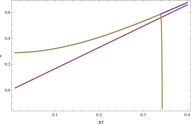
which satisfies the differential equation

y\frac{d^{2}}{dy^{2}}f(y)=\coth y-\frac{1}{y},\quad f(0)=f^{\prime}(0)=0.

(39)

The differential equation may be solved numerically, yielding the results shown in Fig. 11.

V Noncontact gears

We consider first the interaction between corrugated planes, as shown in Fig. 12.

Here we compute the lateral force $F_{\rm lat}$ between the corrugated plates, which are offset by a distance $y_{0}$ . The Dirichlet and electromagnetic cases were previously considered by Emig et al. [33, 34, 35], to second order in corrugation amplitudes. We have carried out the calculations to fourth order [36]. In weak coupling we can calculate to all orders, and verify that fourth order is very accurate, provided $k_{0}h\ll 1$ . We express the lateral force relative to the normal Casimir force between uncorrugated plates, $F_{\rm Cas}^{(0)}$ :

\mathcal{F}=\frac{F_{\rm Lat}}{|F^{(0)}_{\rm Cas}|(h_{1}h_{2}/a^{2})k_{0}a\sin(k_{0}y_{0})}.

(40)

The weak coupling limit is shown in Fig. 13.

V.1 Concentric corrugated cylinders

We can also consider concentric corrugated cylinders, as shown in Fig. 14 [37].

For corrugations given by $\delta$ -function potentials with sinusoidal amplitudes:


$\displaystyle h_{1}(\theta)$	$\displaystyle=$	$\displaystyle h_{1}\sin\nu(\theta+\theta_{0}),$	(41a)
$\displaystyle h_{2}(\theta)$	$\displaystyle=$	$\displaystyle h_{2}\sin\nu\theta,$	(41b)

the torque to lowest order in the corrugations in strong coupling (Dirichlet limit) is

\frac{\tau^{(2)D}}{2\pi RL_{z}}=\nu\sin\nu\theta_{0}\frac{\pi^{2}}{240a^{3}}\frac{h_{1}}{a}\frac{h_{2}}{a}B_{\nu}^{(2)D}(\alpha),\quad\alpha=(a_{2}-a_{1})/(a_{2}+a_{1})\quad R=\frac{1}{2}(a_{1}+a_{2}).

(42)

Figure 15 shows the Dirichlet limit of the torque on cylindrical gears.

A similar result can be found for weak coupling, which, again, has a closed form.

We are currently completing analogous calculations for dielectric materials, illustrated by Fig. 16.

2nd and 4th order results should appear soon, which will complement other recent work [38].

VI Multilayered surfaces

An example of a simple multilayered potential is given in Fig. 17.

To the left of this array of potentials, the reduced Green’s function has the form, in terms of the reflection coefficient $\mathcal{R}$ for the array:

g(x,x^{\prime})=\frac{1}{2\kappa}\left(e^{-\kappa|x-x^{\prime}|}+\mathcal{R}e^{\kappa(x+x^{\prime})}\right),\quad z,z^{\prime}<0.

(43)

(We can actually find the Green’s function everywhere, for any piecewise continuous potential.)

The array reflection coefficient may be readily expressed in terms of the reflection ( $R$ ) and transmission ( $T$ ) coefficients for a single potential:

\mathcal{R}=R+Te^{-\kappa a}\mathcal{R}e^{-\kappa a}(1-Re^{-2\kappa a}\mathcal{R})^{-1},

(44)

where $a=\lambda-d$ is the distance between the potentials, each of thickness $d$ , and the result of summing multiple reflections is

\mathcal{R}=\frac{1}{2R}\bigg[e^{2\kappa a}+R^{2}-T^{2}-\sqrt{\left(e^{2\kappa a}-R^{2}-T^{2}\right)^{2}-4R^{2}T^{2}}\bigg].

(45)

If the potentials consist of dielectric slabs, with dielectric constant $\varepsilon$ and thickness $d$ , the TE reflection and transmission coefficients for a single slab are ( $\kappa^{\prime}=\sqrt{\varepsilon\zeta^{2}+k^{2}}$ )


$\displaystyle R^{\rm TE}$	$\displaystyle=$	$\displaystyle\frac{e^{2\kappa^{\prime}d}-1}{\left(\frac{1+\kappa^{\prime}/\kappa}{1-\kappa^{\prime}/\kappa}\right)e^{2\kappa^{\prime}d}-\left(\frac{1-\kappa^{\prime}/\kappa}{1+\kappa^{\prime}/\kappa}\right)},$	(46a)
$\displaystyle T^{\rm TE}$	$\displaystyle=$	$\displaystyle\frac{4(\kappa^{\prime}/\kappa)e^{\kappa^{\prime}d}}{(1+\kappa^{\prime}/\kappa)^{2}e^{2\kappa^{\prime}d}-(1-\kappa^{\prime}/\kappa)^{2}}.$	(46b)

The TM reflection and transmission coefficients are obtained by replacing, except in the exponents, $\kappa^{\prime}\to\kappa^{\prime}/\varepsilon$ . (Multilayer potentials have been discussed extensively in the past, see, for example, Refs. [39, 40, 41, 28].)

VI.1 Casimir-Polder force

Consider an atom, of polarizability $\alpha(\omega)$ , a distance $Z$ to the left of the array. The Casimir-Polder energy is

E=-\int_{-\infty}^{\infty}d\zeta\int\frac{d^{2}k}{(2\pi)^{2}}\alpha(i\zeta)\mbox{tr}\,{\bf g}(Z,Z),

(47)

where apart from an irrelevant constant the trace is

\mbox{tr}\,{\bf g}(Z,Z)\to\frac{1}{2\kappa}\left[-\zeta^{2}\mathcal{R}^{\rm TE}+(\zeta^{2}+2k^{2})\mathcal{R}^{\rm TM}\right]e^{-2\kappa|Z|}.

(48)

For example, in the static limit, where we disregard the frequency dependence of the polarizability,

E=-\frac{\alpha(0)}{2\pi}\frac{1}{Z^{4}}F(a/Z,d/Z).

(49)

This is compared with the single slab result in Fig. 18.

It is interesting to consider the $Z\to\infty$ limit, which is shown in Fig. 19.

When $a/d\to 0$ we recover the bulk limit.

VII Annular pistons

The multiple scattering approach allows us to calculate the torque between annular pistons, as illustrated in Fig. 20.

We use multiple scattering in the angular coordinates, and an eigenvalue condition in the radial coordinates—the problem is equally well solvable with radial Green’s functions, but this method permits interesting generalizations.

Using the argument principle to determine the angular eigenvalues, we get the following expression for the energy between radial Dirichlet planes for an annular Casimir piston:

	$\displaystyle\mathcal{E}=\frac{E}{L_{z}}$	$\displaystyle=$	$\displaystyle\frac{1}{8\pi^{2}i}\int_{0}^{\infty}{\kappa d\kappa}\int\limits_{\gamma}d\eta\frac{\partial}{\partial\eta}\ln\left[K_{i\eta}(\kappa a)I_{i\eta}(\kappa b)-I_{i\eta}(\kappa a)K_{i\eta}(\kappa b)\right]$		(50)
			$\displaystyle\times\ln\left(1-\frac{\lambda_{1}\lambda_{2}\cosh^{2}\eta(\pi-\alpha)/\cosh^{2}\eta\pi}{\left(2\eta\tanh\eta\pi+\lambda_{1}\right)\left(2\eta\tanh\eta\pi+\lambda_{2}\right)}\right),$		(50)

where $I_{i\eta}$ and $K_{i\eta}$ are modified Bessel functions of imaginary order, and the contour $\gamma$ encircles the poles in $\eta$ along the positive real axis. As to be described elsewhere [42], we have extracted numerical results for the energy, as shown in Fig. 21.

We hope to apply these methods to study interactions between hyperbolæ, such as a hyperbolic cylinder above a plane, and a hyperbola of revolution above a plane, see Figs. 23 and 23.

VIII Conclusions

This survey describes some of the Oklahoma group’s work applying multiple scattering techniques to interesting geometries. We have extensively explored weak coupling, because such cases can be carried out exactly, and therefore they serve as a laboratory for testing general features, such as edge effects and the range of validity of the proximity force approximation. We also have general results for the Green’s functions for arbitrary piecewise continuous potentials in separable coordinates. From these we can calculate not only Casimir-Polder forces, but Casimir energies and torques for many geometries, including annular pistons, and forces between hyperbolic surfaces. Finally, new results for electromagnetic non-contact gears, both for conductors and dielectrics, are in progress.

Acknowledgements.

We thank W.-j. Kim, U. Schwarz, A. Sushkov, and S. Lamoreaux for organizing such a stimulating Workshop on Casimir Forces and Their Measurement. We also acknowledge financial support from the National Science Foundation and the Department of Energy. We thank I. Brevik, S. Ellingsen, and K. Kirsten for collaboration on the annular problem. We especially thank K.V. Shajesh for his contributions to the noncontact gears calculations and the discussion of temperature effects.

References

[1] H. B. G. Casimir, Proc. Kon. Ned. Akad. Wetensch. 51, 793 (1948).
[2] E. M. Lifshitz, Zh. Eksp. Teor. Fiz. 29, 94 (1955) [Sov. Phys. JETP 2, 73 (1956)].
[3] T. H. Boyer, Phys. Rev. 174, 1764 (1968).
[4] L. L. DeRaad, Jr. and K. A. Milton, Ann. Phys. 186, 229 (1981).
[5] B. V. Deryagin (Derjaguin), Kolloid Z. 69, 155 (1934).
[6] M. G. Krein, Mat. Sb. (N.S.) 33, 597 (1953); Dokl. Akad. Nauk SSSR 144, 475 (1962) [Sov. Math. Dokl. 3, 707 (1962)]; M. Sh. Birman and M. G. Krein, Dokl. Akad. Nauk SSSR 144, 268 (1962) [Sov. Math. Dokl. 3, 740 (1962)].
[7] M. J. Renne, Physica 56, 125 (1971).
[8] R. Balian and B. Duplantier, arXiv:quant-ph/0408124, in the proceedings of 15th SIGRAV Conference on General Relativity and Gravitational Physics, Rome, Italy, 9–12 September 2002; Ann. Phys. (N.Y.) 112, 165 (1978); Ann. Phys. (N.Y.) 104, 300 (1977).
[9] A. Wirzba, J. Phys. A 41, 164003 (2008) [arXiv:0711.2395 [quant-ph]].
[10] M. Bordag and V. Nikolaev, J. Phys. A 41, 164002 (2008) [arXiv:0802.3633 [hep-th]].
[11] P. A. Maia Neto, A. Lambrecht, S. Reynaud, Phys. Rev. A 78, 012115 (2008) [arXiv:0803.2444]; A. Canaguier-Durand, P. A. Maia Neto, I. Cavero-Peláez, A. Lambrecht, and S. Reynaud, Phys. Rev. Lett. 102, 230404 (2009) [arXiv:0901.2647].
[12] T. Emig, N. Graham, R. L. Jaffe and M. Kardar, Phys. Rev. Lett. 99, 170403 (2007) [arXiv:0707.1862 [cond-mat.stat-mech]]; Phys. Rev. D 77, 025005 (2008) [arXiv:0710.3084 [cond-mat.stat-mech]]; T. Emig and R. L. Jaffe, J. Phys. A 41, 164001 (2008) [arXiv:0710.5104 [quant-ph]].
[13] S. J. Rahi, T. Emig, N. Graham, R. L. Jaffe, and M. Kardar, arXiv:0908.2649.
[14] M. T. Homer Reid, A. W. Rodriguez, J. White, and S. G. Johnson, Phys. Rev. Lett. 103, 040401 (2009) [arXiv:0904.0741].
[15] K. A. Milton and J. Wagner, J. Phys. A 41, 155402 (2008) [arXiv:0712.3811 [hep-th]].
[16] K. A. Milton, J. Phys. Conf. Ser. 161, 012001 (2009) [arXiv:0809.2564 [hep-th]].
[17] H. Gies and K. Klingmüller, Phys. Rev. D 74, 045002 (2006) [arXiv:quant-ph/0605141].
[18] H. Gies and K. Klingmüller, Phys. Rev. Lett. 96, 220401 (2006) [arXiv:quant-ph/0601094].
[19] H. Gies and K. Klingmüller, Phys. Rev. Lett. 97, 220405 (2006) [arXiv:quant-ph/0606235].
[20] H. Gies, K. Langfeld and L. Moyaerts, JHEP 0306, 018 (2003) [arXiv:hep-th/0303264].
[21] A. Rodriguez, M. Ibanescu, D. Iannuzzi, F. Capasso, J. D. Joannopoulos, and S. G. Johnson, Phys. Rev. Lett. 99, 080401 (2007) [arXiv:0704.1890v2].
[22] A. Rodriguez, M. Ibanescu, D. Iannuzzi, J. D. Joannopoulos, and S. G. Johnson, Phys. Rev. A 76, 032106 (2007) [arXiv:0705.3661].
[23] A. W. Rodriguez, J. D. Joannopoulos, and S. G. Johnson, Phys. Rev. A 77, 062107 (2008) [arXiv:0802.1494].
[24] J. Wagner, K. A. Milton and P. Parashar, J. Phys. Conf. Ser. 161, 012022 (2009) [arXiv:0811.2442 [hep-th]].
[25] S. A. Fulling, L. Kaplan, K. Kirsten, Z. H. Liu, and K. A. Milton, J. Phys. A: Math. Theor. 42, 155402 (2009) [arXiv:0806.2468 [hep-th]].
[26] H. B. G. Casimir and D. Polder, Phys. Rev. 73, 360 (1948).
[27] K. A. Milton, P. Parashar and J. Wagner, Phys. Rev. Lett. 101, 160402 (2008) [arXiv:0806.2880 [hep-th]].
[28] V. A. Parsegian, Van der Waals Forces: A Handbook for Biologists, Chemists, Engineers, and Physicists (Cambridge University Press, 2006).
[29] T. H. Boyer, Phys. Rev. A 9, 2078 (1974).
[30] K. A. Milton, P. Parashar and J. Wagner, The Casimir effect and cosmology, ed. S. D. Odintsov, E. Elizalde, and O. B. Gorbunova, in honor of Iver Brevik (Tomsk State Pedagogical University) pp. 107-116 (2009) [arXiv:0811.0128 [math-ph]].
[31] K. A. Milton, P. Parashar, J. Wagner and K. V. Shajesh, arXiv:0909.0977 [hep-th].
[32] R. S. Decca, E. Fischbach, G. L. Klimchitskaya, D. E. Krause, D. Lopez and V. M. Mostepanenko, Phys. Rev. D 79, 124021 (2009) [arXiv:0903.1299 [quant-ph]].
[33] T. Emig, A. Hanke, R. Golestanian, and M. Kardar, Phys. Rev. Lett. 87, 260402 (2001) [arXiv:cond-mat/0106028].
[34] T. Emig, A. Hanke, R. Golestanian and M. Kardar, Phys. Rev. A 67, 022114 (2003) [arXiv:cond-mat/0211193].
[35] R. Büscher and T. Emig, Phys. Rev. A 69, 062101 (2004) [arXiv:cond-mat/0401451].
[36] I. Cavero-Peláez, K. A. Milton, P. Parashar and K. V. Shajesh, Phys. Rev. D 78, 065018 (2008) [arXiv:0805.2776 [hep-th]].
[37] I. Cavero-Peláez, K. A. Milton, P. Parashar and K. V. Shajesh, Phys. Rev. D 78, 065019 (2008) [arXiv:0805.2777 [hep-th]].
[38] A. Lambrecht and V. N. Marachevsky, Phys. Rev. Lett. 101, 160403 (2008) [arXiv:0806.3142].
[39] F. Zhou and L. Spruch, Phys. Rev. A 52, 297 (1995).
[40] M. S. Tomaš, Phys. Rev. A 66, 052103 (2002) [arXiv:quant-ph/0207106].
[41] M. Bordag, G. Klimchitskaya, U. Mohideen, and V. M. Mostepanenko, Advances in the Casimir Effect (Oxford University Press, 2009).
[42] K. A. Milton, J. Wagner, and K. Kirsten, “Casimir Effect for a Semitransparent Wedge,” in preparation.