GRB 081028 and its late-time afterglow re-brightening

GRB 081028 and its late-time afterglow re-brightening–22009

R. Margutti ^†^†thanks: E-mail: raffaella.margutti@brera.inaf.it (RM) Affiliation: Università degli studi Milano Bicocca, P.za della Scienza 3, Milano 20126, Italy Affiliation: INAF Osservatorio Astronomico di Brera, via Bianchi 46, Merate 23807, Italy F. Genet Affiliation: Centre for Astrophysics Research, University of Hertfordshire, UK J. Granot Affiliation: Centre for Astrophysics Research, University of Hertfordshire, UK R. Barniol Duran Affiliation: Department of Physics, University of Texas at Austin, Austin, TX 78712, USA C. Guidorzi Affiliation: INAF Osservatorio Astronomico di Brera, via Bianchi 46, Merate 23807, Italy Affiliation: Dipartimento di Fisica, Università di Ferrara, via Saragat 1, 44100 Ferrara, Italy G. Chincarini Affiliation: Università degli studi Milano Bicocca, P.za della Scienza 3, Milano 20126, Italy Affiliation: INAF Osservatorio Astronomico di Brera, via Bianchi 46, Merate 23807, Italy J. Mao Affiliation: INAF Osservatorio Astronomico di Brera, via Bianchi 46, Merate 23807, Italy Affiliation: Yunnan Observatory, Chinese Academy of Sciences, P.O. Box 110, Kunming, Yunnan Province, China P. Schady Affiliation: The UCL Mullard Space Science Laboratory, Holmbury St Mary, Dorking, Surrey RH5 6NT T. Sakamoto Affiliation: NASA Goddard Space Flight Center, Greenbelt, MD 20771 A. A. Miller Affiliation: Department of Astronomy, University of California, Berkeley, CA 94720-3411, USA G. Olofsson Affiliation: Stockholm Observatory, Stockholm University, Astronomy Department AlbaNova Research Center, 106 91 Stockholm, Sweden J.S. Bloom Affiliation: Department of Astronomy, University of California, Berkeley, CA 94720-3411, USA P.A. Evans Affiliation: X-ray and Observational Astronomy Group, Department of Physics and Astronomy, University of Leicester, LE1 7RH, UK J.P.U. Fynbo Affiliation: Dark Cosmology Centre, Niels Bohr Institute, University of Cøpenhagen, Juliane MariesVej 30, 2100 Copenhagen O, Denmark D. Malesani Affiliation: Dark Cosmology Centre, Niels Bohr Institute, University of Cøpenhagen, Juliane MariesVej 30, 2100 Copenhagen O, Denmark A. Moretti Affiliation: INAF Osservatorio Astronomico di Brera, via Bianchi 46, Merate 23807, Italy F. Pasotti Affiliation: INAF Osservatorio Astronomico di Brera, via Bianchi 46, Merate 23807, Italy D. Starr Affiliation: Department of Astronomy, University of California, Berkeley, CA 94720-3411, USA D.N. Burrows Affiliation: Department of Astronomy and Astrophysics, Pennsylvania State University, 525 Davey Lab, University Park, PA 16802 S.D. Barthelmy Affiliation: NASA Goddard Space Flight Center, Greenbelt, MD 20771 P.W.A. Roming Affiliation: Department of Astronomy and Astrophysics, Pennsylvania State University, 525 Davey Lab, University Park, PA 16802 N. Gehrels Affiliation: NASA Goddard Space Flight Center, Greenbelt, MD 20771

Accepted 200? Month Day Received 2009 Month Day; in original form 2009 March 19

Abstract

Swift captured for the first time a smoothly rising X-ray re-brightening of clear non-flaring origin after the steep decay in a long gamma-ray burst (GRB): GRB 081028. A rising phase is likely present in all GRBs but is usually hidden by the prompt tail emission and constitutes the first manifestation of what is later to give rise to the shallow decay phase. Contemporaneous optical observations reveal a rapid evolution of the injection frequency of a fast cooling synchrotron spectrum through the optical band, which disfavours the afterglow onset (start of the forward shock emission along our line of sight when the outflow is decelerated) as the origin of the observed re-brightening. We investigate alternative scenarios and find that the observations are consistent with the predictions for a narrow jet viewed off-axis. The high on-axis energy budget implied by this interpretation suggests different physical origins of the prompt and (late) afterglow emission. Strong spectral softening takes place from the prompt to the steep decay phase: we track the evolution of the spectral peak energy from the $\gamma$ -rays to the X-rays and highlight the problems of the high latitude and adiabatic cooling interpretations. Notably, a softening of both the high and low spectral slopes with time is also observed. We discuss the low on-axis radiative efficiency of GRB 081028 comparing its properties against a sample of Swift long GRBs with secure $E_{\rm{\gamma,iso}}$ measurements.

Keywords:

gamma-ray: bursts – radiation mechanism: non-thermal –X-rays: individual (GRB081028).

1 Introduction

Gamma ray bursts (GRBs) are transient events able to outshine the $\gamma$ -ray sky for a few seconds to a few minutes. The discovery of their optical (van Paradijs et al.,, 1997) and X-ray (Costa et al., 1997) long-lasting counterparts represented a breakthrough for GRB science. Unfortunately, due to technological limitations, the X-ray observations were able to track the afterglow evolution starting hours after the trigger: only after the launch of the Swift satellite in 2004 (Gehrels et al., 2004) was this gap between the end of the prompt emission and several hours after the onset of the explosion filled with X-ray observations. A canonical picture was then established (see e.g., Nousek et al. 2006), with four different stages describing the overall structure of the X-ray afterglows: an initial steep decay, a shallow-decay phase, a normal decay and a jet-like decay stage. Erratic flares are found to be superimposed mainly to the first and second stage of emission. An interesting possibility is that the four light-curve phases instead belong to only two different components of emission (see e.g., Willingale et al. 2007): the first, connected to the activity of the central engine giving rise to the prompt emission, comprises the flares (Chincarini et al. 2007 and references therein) and the steep-decay phase; the second is instead related to the interaction of the outflow with the external medium and manifests itself in the X-ray regime through the shallow, normal and jet-like decay. Observations able to further characterise the two components are therefore of particular interest.

The smooth connection of the X-ray steep decay light-curve phase with the prompt $\gamma$ -ray emission strongly suggests a common physical origin (Tagliaferri et al. 2005; O’Brien et al. 2006): the high latitude emission (HLE) model (Fenimore et al. 1996; Kumar & Panaitescu 2000) predicts that steep decay photons originate from the delay in the arrival time of prompt emission photons due to the longer path length from larger angles relative to our line of sight, giving rise to the $\alpha=\beta+2$ relation (where $\alpha$ is the light-curve decay index and $\beta$ is the spectral energy index). No spectral evolution is expected in the simplest formulation of the HLE effect in the case of a simple power-law prompt spectrum. Observations say the opposite: significant variations of the photon index have been found in the majority of GRBs during the steep decay phase (see e.g., Zhang, Liang & Zhang 2007); more than this, the absorbed simple power-law (SPL) has proved to be a poor description of the spectral energy distribution of the steep decay phase for GRBs with the best statistics¹¹ 1 The limited $0.3-10\,\rm{keV}$ spectral coverage of the Swift X-Ray Telescope, XRT (Burrows et al., 2005), and the degeneracy between the variables of the spectral fit can in principle lead to the identification of an SPL behaviour in intrinsically non-SPL spectra with poor statistics.. A careful analysis of these events has shown their spectra to be best fit by an evolving Band function (Band et al., 1993), establishing the link between steep decay and prompt emission photons also from the spectral point of view (see e.g., GRB 060614, Mangano et al. 2007; GRB 070616, Starling et al. 2008): caused by the shift of the Band spectrum, a temporal steep decay phase and a spectral softening appear simultaneously (see e.g. Zhang, Liang & Wang 2009, Qin et al. 2009). In particular, the peak energy of the $\nu F_{\nu}$ spectrum is found to evolve to lower values, from the $\gamma$ -ray to the soft X-ray energy range. Both the low (as observed for GRB 070616) and the high-energy portion of the spectrum are likely to soften with time, but no observation is reported to confirm the high energy index behaviour during the prompt and steep decay phase. The observed spectral evolution with time is an invaluable footprint of the physical mechanisms at work: observations able to constrain the behaviour of the spectral parameters with time are therefore of primary importance.

By contrast, no spectral evolution is observed in the X-ray during the shallow decay phase (see e.g. Liang, Zhang & Zhang 2007) experienced by most GRBs between $\sim 10^{2}$ s and $10^{3}-10^{4}$ s. An unexpected discovery of the Swift mission, the shallow decay is the first light-curve phase linked to the second emission component. A variety of theoretical explanations have been put forward. The proposed models include: energy injection (Panaitescu et al. 2006; Rees & Meszaros 1998; Granot & Kumar 2006; Zhang et al. 2006); reverse shock (see e.g., Genet, Daigne & Mochkovitch 2007); time dependent micro-physical parameters (see e.g. Granot, Königl & Piran 2006; Ioka et al. 2006); off-axis emission (Eichler & Granot, 2006); dust scattering (Shao & Dai, 2007). The predictions of all these models can only be compared to observations tracking the flat and decay phase of the second emission component, since its rise is usually missed in the X-ray regime, being hidden by the tail of the prompt emission.

GRB 081028 is the first and unique event for which Swift was able to capture the rise of the second emission component²² 2 There are a handful of long GRBs detected by Swift with a possible X-ray rise of non-flaring origin. Among them: GRB 070328, Markwardt et al. (2007); GRB 080229A, Cannizzo et al. (2008); GRB 080307, Page et al. (2009) (see Page et al. 2009 and references therein). However, in none of these cases has an X-ray steep decay been observed. A smooth rise in the X-rays has been observed in the short GRB 050724.: the time properties of its rising phase can be constrained for the first time while contemporaneous optical observations allow us to track the evolution of a break energy of the spectrum through the optical band. GRB 081028 is also one of the lucky cases showing a spectrally evolving prompt emission where the evolution of the spectral parameters can be studied from $\gamma$ -rays to X-rays, from the trigger time to $\sim 1000$ s. A hard to soft spectral evolution is clearly taking place beginning with the prompt emission and extending to the steep decay phase, as already found for other Swift GRBs (GRB 060614, Mangano et al. 2007; GRB 070616, Starling et al. 2008, are showcases in this respect). Notably, for GRB 081028 a softening of the slope of a Band function (Band et al., 1993) above $E_{\rm p}$ is also observed.

The paper is organised as follows: Swift and ground-based observations are described in Sect. 2; data reduction and preliminary analysis are reported in Sect. 3, while in Sect. 4 the results of a detailed spectral and temporal multi-wavelength analysis are outlined and discussed in Sect. 5. Conclusions are drawn in Sect. 6.

The phenomenology of the burst is presented in the observer frame unless otherwise stated. The convention $F_{\nu}(\nu,t)\propto\nu^{-\beta}t^{-\alpha}$ is followed, where $\beta$ is the spectral energy index, related to the spectral photon index $\Gamma$ by $\Gamma=\beta+1$ . All the quoted uncertainties are given at 68% confidence level (c.l.): a warning is added if it is not the case. The convention $Q_{x}=Q/10^{x}$ has been adopted in cgs units unless otherwise stated. Standard cosmological quantities have been adopted: $H_{0}=70\,\rm{km\,s^{-1}\,Mpc^{-1}}$ , $\Omega_{\Lambda}=0.7$ , $\Omega_{\rm{M}}=0.3$ .

2 Observations

GRB 081028 triggered the Swift Burst Alert Telescope (BAT; Barthelmy et al. 2005) on 2008-10-28 at 00:25:00 UT (Guidorzi et al., 2008). The spacecraft immediately slewed to the burst allowing the X-ray Telescope (XRT; Burrows et al. 2005) to collect photons starting at $T+191\,\rm{s}$ after the trigger: a bright and fading X-ray afterglow was discovered. The UV/Optical Telescope (UVOT, Roming et al. 2005) began observing at $T+210\,\rm{s}$ . In the first orbit of observations, no afterglow candidate was detected in any of the UVOT filters in either the individual or co-added exposures. A careful re-analysis of the acquired data revealed the presence of a source with a White band magnitude of $20.9$ at $\sim T+270\,\rm{s}$ (this paper). A refined position was quickly available thanks to the XRT-UVOT alignment procedure and the match of UVOT field sources to the USNO-B1 catalogue (see Goad et al. 2007 for details): R.A.(J2000)= $08^{\rm{h}}07^{\rm{m}}34.76^{\rm{s}}$ , Dec.(J2000)= $+02^{\circ}18^{\prime}29.8″$ with a 90% error radius of 1.5 arcsec (Evans et al., 2008). Starting at $\sim T+9\,\rm{ks}$ the X-ray light-curve shows a remarkable re-brightening (Guidorzi et al., 2008b), see Fig. 2: this was later detected in ground-based near-infrared (NIR) and optical observations. Preliminary analysis results for this burst were reported in Guidorzi et al. (2008c).

The Telescope a Action Rapide pour les Objets Transitoires (TAROT; Klotz et al. 2008) began observing $566.4\,\rm{s}$ after the trigger under poor weather conditions: no variable source was detected down to $R\sim 17.4$ .

The optical afterglow was discovered by the Gamma-Ray Burst Optical and Near-Infrared Detector (GROND; Greiner et al. 2008). The observations started 20.9 ks after the trigger: the afterglow was simultaneously detected in the $g^{\prime}r^{\prime}i^{\prime}z^{\prime}JHK$ bands (Clemens et al., 2008) with the following preliminary magnitudes: $g^{\prime}=19.9\pm{0.1}$ ; $r^{\prime}=19.3\pm{0.1}$ ; $i^{\prime}=19.2\pm{0.1}$ ; $z^{\prime}=19.1\pm{0.1}$ ; $J=19.0\pm{0.15}$ ; $H=18.7\pm{0.15}$ ; $K=19.0\pm{0.15}$ , with a net exposure of $264$ and $240\,\rm{s}$ for the $g^{\prime}r^{\prime}i^{\prime}z^{\prime}$ and the $JHK$ bands respectively. Further GROND observations were reported by Clemens et al. (2008b) $113\,\rm{ks}$ after the trigger with $460\,\rm{s}$ of total exposures in $g^{\prime}r^{\prime}i^{\prime}z^{\prime}$ and $480\,\rm{s}$ in $JHK$ . Preliminary magnitudes are reported below: $g^{\prime}=21.26\pm{0.05}$ ; $r^{\prime}=20.49\pm{0.05}$ ; $i^{\prime}=20.24\pm{0.05}$ ; $z^{\prime}=19.99\pm{0.05}$ ; $J=19.6\pm{0.1}$ . The source showed a clear fading with respect to the first epoch, confirming its nature as a GRB afterglow.

The Nordic Optical Telescope (NOT) imaged the field of GRB 081028 $\sim 6\,\rm{hr}$ after the trigger and independently confirmed the optical afterglow with a magnitude $R\sim 19.2$ (Olofsson et al., 2008). Because of the very poor sky conditions only 519 frames out of 9000 could be used, with a total exposure of 51.9 s. The average time for the observations is estimated to be 05:53:00 UT. Image reduction was carried out by following standard procedures.

An UV/optical re-brightening was discovered by the UVOT starting $T+10\,\rm{ks}$ , simultaneous to the X-ray re-brightening. The afterglow was detected in the $v$ , $b$ and $u$ -band filters (Shady et al., 2008). The UVOT photometric data-set of GRB 081028 is reported in Tab. 1. We refer to Poole et al. (2008) for a detailed description of the UVOT photometric system.

The rising optical afterglow was independently confirmed by the Crimean telescope for Asteroid Observations (CrAO) and by the Peters Automated Infrared Imaging Telescope (PAIRITEL; Bloom et al. 2006). CrAO observations were carried out starting at $\sim T+1\,\rm{ks}$ and revealed a sharp rising optical afterglow peaking after $T+9.4\,\rm{ks}$ : $R=21.62\pm 0.07$ at $t=T+1.8\,\rm{ks}$ ; $I=21.32\pm 0.09$ at $t=T+3.6\,\rm{ks}$ ; $I=21.43\pm 0.09$ at $t=T+5.5\,\rm{ks}$ ; $I=21.20\pm 0.08$ at $t=T+7.5\,\rm{ks}$ ; $I=20.66\pm 0.05$ at $t=T+9.4\,\rm{ks}$ (Rumyantsev et al., 2008).

PAIRITEL observations were carried out $40\,\rm{ks}$ after the trigger: the afterglow was simultaneously detected in the $J$ , $H$ , and $K_{\rm{s}}$ filters with a preliminary photometry $J=17.7\pm 0.1$ , $H=17.0\pm 0.1$ and $K_{\rm{s}}=16.1\pm 0.1$ (Miller et al., 2008). A total of 472 individual 7.8 s exposures were obtained under bad conditions (seeing $\ga$ 3^′′) for a total exposure time of $\sim$ 3682 s. The data were reduced and analysed using the standard PAIRITEL pipeline (Bloom et al., 2006). Photometry calibration was done against the 2MASS system. The resulting fluxes and magnitudes are consistent with the values reported by Miller et al. (2008): however, this work should be considered to supersede the previous findings. The ground-based photometric data-set of GRB 081028 is reported in Tab. 2 while the photometric optical observations of GRB 081028 are portrayed in Fig. 2.

A spectrum of the GRB 081028 afterglow was taken with the Magellan Echellette Spectrograph (MagE) on the Magellan/Clay 6.5-m telescope at $\sim T+27\,\rm{ks}$ for a total integration time of $1.8\,\rm{ks}$ . The identification of absorption features including SII, NV, SiIV, CIV and FeII allowed the measurement of the redshift $z=3.038$ together with the discovery of several intervening absorbers (Berger et al., 2008).

According to Schlegel et al. (1998) the Galactic reddening along the line of sight of GRB 081028 is $E(B-V)=0.03$ .

3 Swift Data Reduction and preliminary analysis

Refer to caption — Figure 1: Top panel: BAT 15-150 keV mask weighted light-curve (binning time of 4.096 s). Solid blue line: $15-150\,\rm{keV}$ light-curve best fit using Norris et al. (2005) profiles. The typical $1~\sigma$ error size is also shown. Bottom panel: best fit photon index $\Gamma_{\gamma}$ as a function of time (errors are provided at the 90% c.l.).

The BAT data have been processed using standard Swift-BAT analysis tools within heasoft (v.6.6.1). The ground-refined coordinates provided by Barthelmy et al. (2008) have been adopted in the following analysis. Standard filtering and screening criteria have been applied. The mask-weighted background subtracted $15-150\,\rm{keV}$ is shown in Fig. 1, top panel. The mask-weighting procedure is also applied to produce weighted, background subtracted counts spectra. Before fitting the spectra, we group the energy channels requiring a 3- $\sigma$ threshold on each group; the threshold has been lowered to 2- $\sigma$ for spectra with poor statistics. The spectra are fit within Xspec v.12.5 with a simple power-law with pegged normalisation (pegpwrlw). The best fit photon indices resulting from this procedure are shown in Fig. 1, bottom panel.

XRT data have also been processed with heasoft (v. 6.6.1) and corresponding calibration files: standard filtering and screening criteria have been applied. The first orbit data were acquired entirely in WT mode reaching a maximum count rate $\sim 140\,\rm{counts\,s^{-1}}$ . We apply standard pile-up corrections following the prescriptions of Romano et al. (2006) when necessary. Starting from $\sim 10\,\rm{ks}$ Swift-XRT switched to PC mode to follow the fading of the source: events are then extracted using different region shapes and sizes in order to maximize the signal-to-noise (SN) ratio. The background is estimated from a source free portion of the sky. The resulting X-ray light-curve is shown in Fig. 2: the displayed data binning assures a minimum SN equals to 4 (10) for PC (WT) data. In this way the strong variability of WT data can be fully appreciated without losing information on the late time behaviour. We perform automatic time resolved spectral analysis, accumulating signal over time intervals defined to contain a minimum of $\sim 2000$ photons each. The spectral channels have been grouped to provide a minimum of 20 counts per bin. The Galactic column density in the direction of the burst is estimated to be $3.96\times 10^{20}\,\rm{cm^{-2}}$ (weighted average value from the Kalberla et al. 2005 map). Spectral fitting is done within Xspec (v.12.5) using a photo-electrically absorbed simple power law (SPL) model. The Galactic absorption component is frozen at the Galactic value together with the redshift, while we leave the intrinsic column density free to vary during the first run of the program. A count-to-flux conversion factor is worked out from the best fit model for each time interval for which we are able to extract a spectrum. This value is considered reliable if the respective $\chi^{2}/\rm{dof}$ (chi-square over degrees of freedom) implies a P-value (probability of obtaining a result at least as extreme as the one that is actually observed) higher than 5%. The discrete set of reliable count-to-flux conversion factors is then used to produce a continuous count-to-flux conversion factor through interpolation. This procedure produces flux and luminosity light-curves where the possible spectral evolution of the source is properly taken into account (Fig. 2). In the case of GRB 081028 this is particularly important: the simple power law photon index evolves from $\Gamma\sim 1.2$ to $\Gamma\sim 3$ during the steep decay phase (Fig. 6), inducing a variation of a multiplicative factor $\sim 1.7$ in the count-to-flux conversion factor. As a second run, we remove one degree of freedom from the spectral fitting procedure, noting the absence of spectral evolution during the X-ray re-brightening in the X-ray regime (see Sect. 4.4). This gives the possibility to obtain a reliable estimate of the intrinsic neutral Hydrogen column density $N_{\rm{H,z}}$ of GRB 081028: the PC spectrum accumulated over the time interval $10-652\,\rm{ks}$ can be adequately fit by an absorbed SPL model with best fit photon index $\Gamma=2.09\pm 0.07$ and $N_{\rm{H,z}}=(0.52\pm 0.25)\times 10^{22}\,\rm{cm^{-2}}$ ( $90\%$ c.l. uncertainties are provided). The flux-luminosity calibration procedure is then re-run freezing the intrinsic absorption component to this value.

The UVOT photometry was performed using standard tools (Poole et al., 2008) and is detailed in Tab. 1.

4 Analysis and results

4.1 Temporal analysis of BAT (15-150 keV) data

	Pulse 1	Pulse 2
$t_{\rm{peak}}$ (s)	$72.3\pm 3.5$	$202.7\pm 3.3$
$t_{\rm{s}}$ (s)	$5.4\pm 17.5$	$125.6\pm 18.1$
$t_{\rm{rise}}$ (s)	$32.6\pm 3.7$	$36.4\pm 4.1$
$t_{\rm{decay}}$ (s)	$63.4\pm 8.1$	$70.0\pm 5.2$
$w$ (s)	$96.0\pm 7.9$	$105.4\pm 6.2$
$k$	$0.32\pm 0.09$	$0.31\pm 0.07$
$A$ ( $\rm{count\,\,\rm{s^{-1}}}\,\rm{det^{-1}}$ )	$(3.6\pm 0.2)10^{-2}$	$(3.5\pm 0.2)10^{-2}$
Fluence ( $\rm{erg\,\,cm^{-2}}$ )	$(1.81\pm 0.14)10^{-6}$	$(1.83\pm 0.11)10^{-6}$
$\chi^{2}/\rm{dof}$	171/114

Table 1: Best fit parameters and related quantities resulting from the modelling of the prompt 15-150 keV emission with two Norris et al. (2005) profiles. From top to bottom: peak time, start time,

1/e

rise time,

1/e

decay time,

1/e

pulse width, pulse asymmetry, peak count-rate and statistical information. The

\chi^{2}

value mainly reflects the partial failure of the fitting function to adequately model the peaks of the pulses (see Norris et al. 2005 for details).

The mask-weighted light-curve consists of two main pulses peaking at $T+70\,\rm{s}$ and $\sim T+200\,\rm{s}$ followed by a long lasting tail out to $\sim T+400\,\rm{s}$ . In the time interval $T-100\,\rm{s}$ $T+400\,\rm{s}$ , the light-curve can be fit by a combination of two Norris et al. (2005) profiles (Fig. 1, top panel), each profile consisting of the inverse of the product of two exponentials, one increasing and one decreasing with time. The best fit parameters and related quantities are reported in Table 1: the parameters are defined following Norris et al. (2005); we account for the entire covariance matrix during the error propagation procedure. The GRB prompt signal has a $T_{90}$ duration of $261.0\pm 28.7$ s and a $T_{50}=128.2\pm 7.7$ s.

The temporal variability of this burst has been characterised in two different ways. First, following Rizzuto et al. (2007) we compute a variability measure $\rm{Var}(15-150\,\rm{keV})=(5.0\pm 0.14)\times 10^{-2}$ . Second, we adopt the power spectrum analysis in the time domain (Li 2001; Li et al. 2002): unlike the Fourier spectrum, this is suitable to study the rms variations at different time-scales. See Margutti et al. (2008) and Margutti et al. in prep. for details about the application of this technique to the GRB prompt emission. In particular, we define the fractional power density (fpd) as the ratio between the temporal power of the source signal and the mean count rate squared. This quantity is demonstrated to show a peak at the characteristic time scales of variability of the signal. We assess the significance of each fpd peak via Montecarlo simulations. The fpd of GRB 081028 shows a clear peak around 70 s (time scale related to the width of the two Norris et al. 2005 profiles). Below 70 s the fpd shows a first peak at $\Delta t\sim 2\,\rm{s}$ and then a second peak at $\Delta t\sim 6\,\rm{s}$ , both at 1- $\sigma$ c.l. The signal shows power in excess of the noise at 2- $\sigma$ c.l. significance for time scales $\Delta t\geq 32\,\rm{s}$ .

4.2 Spectral analysis of BAT (15-150 keV) data

Interval	Model	$t_{\rm{start}}$	$t_{\rm{stop}}$	$\Gamma,\alpha$	$E_{\rm{p}}$	Fluence	$\chi^{2}/\rm{dof}$	P-value
		(s)	(s)		(keV)	( $\rm{erg\,cm^{-2}}$ )
$T_{90}$	Pl	52.9	317.2	$1.82\pm 0.09$	–	$(3.3\pm 0.20)\times 10^{-6}$	$31.8/31$	$43\%$
	Cutpl	52.9	317.2	$1.3\pm 0.4$	$65^{+42}_{-11}$	$(3.15\pm 0.20)\times 10^{-6}$	$25.8/30$	$69\%$
Total	Pl	0.0	400.0	$1.89\pm 0.09$	–	$(3.7\pm 0.20)\times 10^{-6}$	$37.4/32$	$23\%$
	Cutpl	0.0	400.0	$1.3\pm 0.4$	$55^{+20}_{-9}$	$(3.45\pm 0.19)\times 10^{-6}$	$30.1/31$	$51\%$
Pulse 1	Pl	10.0	150.0	$1.91\pm 0.13$	–	$(1.60\pm 0.12)\times 10^{-6}$	$18.0/24$	$80\%$
	Cutpl	10.0	150.0	$1.1\pm 0.6$	$49^{+18}_{-9}$	$(1.47\pm 0.11)\times 10^{-6}$	$12.0/23$	$97\%$
Pulse 2	Pl	150.0	290.0	$1.77\pm 0.11$	–	$(1.79\pm 0.11)\times 10^{-6}$	$33.8/29$	$25\%$
	Cutpl	150.0	290.0	$1.22\pm 0.45$	$69^{+87}_{-14}$	$(1.47\pm 0.11)\times 10^{-6}$	$29.3/28$	$40\%$

Table 2: Best fit parameters derived from the spectral modelling of 15-150 keV data using a power law with pegged normalisation (Pl, pegpwrlw within Xspec) and a cut-off power-law model with the peak energy of the

\nu F_{\nu}

spectrum as free parameter (Cutpl). From left to right: name of the interval of the extraction of the spectrum we refer to throughout the paper; spectral model used; start and stop times of extraction of the spectrum; best fit photon index

\Gamma

for a Pl model or cutoff power-law index for a Cutpl model; best fit peak energy of the

\nu F_{\nu}

spectrum; fluence; statistical information about the fit.

We extract several spectra in different time intervals and then fit the data using different models to better constrain the spectral evolution of GRB 081028 in the 15-150 keV energy band. The first spectrum is extracted during the $T_{90}$ duration of the burst; a second spectrum is accumulated during the entire duration of the 15-150 keV emission; finally, the signal between 10 s and 290 s from trigger has been split into two parts, taking 150 s as dividing time, to characterise the spectral properties of the two prompt emission pulses. The resulting spectra are then fit using a simple power-law and a cut-off power-law models within Xspec. The results are reported in Table 2. The measured simple power law photon index around 2 suggests that BAT observed a portion of an intrinsically Band spectrum (Band et al., 1993). Consistent with this scenario, the cut-off power law model always provides a better fit which is able to constrain the peak energy value ( $E_{\rm{p}}$ , peak of the $\nu F_{\nu}$ spectrum) within the BAT energy range.

The best fit parameters of the cut-off power-law model applied to the total spectrum of Table 2 imply $E_{\rm{iso,\gamma}}(1-10^{4}\,\rm{keV})=(1.1\pm 0.1)\times 10^{53}\,\rm{erg}$ . The respective rest frame peak energy is $E_{\rm{p,i}}=(1+z)E_{\rm{p}}=222^{+81}_{-36}\,\rm{keV}$ , placing GRB 081028 within the 2- $\sigma$ region of the Amati relation (Amati, 2006). The burst is characterised by an isotropic $10^{2}-10^{3}$ keV (rest frame) $L_{\rm{iso}}=(2.85\pm 0.25)\times 10^{51}\,\rm{erg\,s^{-1}}$ . This information together with the variability measure $\rm{Var}(15-150\,\rm{keV})=(5.0\pm 0.14)\times 10^{-2}$ makes GRB 081028 perfectly consistent with the luminosity variability relation (see Reichart et al. 2001; Guidorzi et al. 2005; Rizzuto et al. 2007).

4.3 Temporal analysis of XRT (0.3-10 keV) data

$n_{2}$	$c$	$n_{1}$	$a$	$b$	$d_{1}$	$t_{\rm{br}_{1}}$	$n_{3}$	$e$	$d_{2}$	$t_{\rm{br}_{2}}$	$\chi^{2}/\rm{dof}$
						(ks)				(ks)
$10^{18.3\pm 5.5}$	$-5.2\pm 1.5$	$1.2\pm 1.1$	$-4.5\pm 3.3$	$2.1\pm 0.1$	$2.4\pm 2.0$	$15.5\pm 6.3$	$-$	$-$	$-$	$-$	$164.8/145$
$10^{29.9\pm 6.5}$	$-7.60\pm 1.8$	$0.31\pm 0.02$	$-1.8\pm 0.3$	$1.3\pm 0.1$	$0.1$	$19.5\pm 0.7$	$0.06$	$2.3\pm 0.1$	$0.05$	62	$147.1/143$

Table 3: Best-fit parameters of the XRT light-curve modelling starting from 3 ks after the trigger. The first (second) line refers to Eq. 1 (Eq. 2).

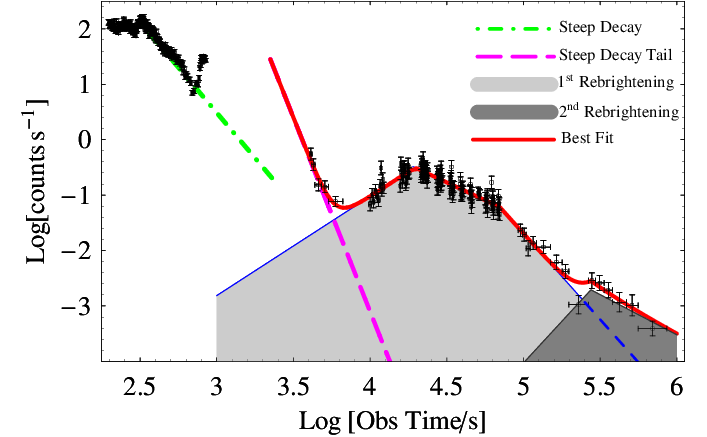
The XRT (0.3-10 keV) light-curve consists of two parts: a steep decay phase with flares and variability superimposed ( $100\,\rm{s}<t<7000\,\rm{s}$ ), followed by a remarkable re-brightening with smoothly rising and decaying emission between 7 ks and $1000\,\rm{ks}$ . The two light-curve phases are studied separately.

GRB 081028 is one of the rare cases in which the XRT caught the prompt emission. The light-curve shows a flat phase up to $t\sim 300\,\rm{s}$ followed by a steep decay. Starting from $\sim 690\,\rm{s}$ the light-curve is dominated by a flare which peaks at 800 s but whose decaying phase is temporally coincident with the orbital data gap. The steep decay behaviour before the flare is inconsistent with the back-extrapolation of the post orbital data gap power-law decay, as shown in Fig. 3. The strong spectral evolution detected by the XRT (Sect. 4.4) requires a time resolved flux calibration of the light-curve before the light-curve fitting procedure. In the time interval $320\,\rm{s}<t<685\,\rm{s}$ the 0.3-10 keV light-curve best fit is given by a simple power-law with $\alpha=3.6\pm 0.1$ ( $\chi^{2}/\rm{dof}=768.3/736$ ). Figure 4 shows the different temporal behaviour of the detected signal when split into different energy bands: harder photons decay faster. The 0.3-1 keV light-curve decays following a power-law with index $\alpha\approx-2.5$ ; the decay steepens to $\alpha\approx-3.5$ and $\alpha\approx-3.8$ for the 1-2 keV and 2-10 keV signal, respectively.

During the re-brightening there is no evidence for spectral evolution in the XRT energy band (see Sect. 4.4). For this reason we model the count-rate light-curve instead of the flux calibrated one: this gives the possibility to obtain a fully representative set of best fit parameters³³ 3 This is in general not true in cases of strong spectral evolution as shown in the first part of this section. determined with the highest level of precision. The count-to-flux calibration introduces additional uncertainty inherited by the spectral fitting procedure. Starting from 3 ks (the inclusion of the last part of the steep decay is necessary to model the rising part of the re-brightening), the count-rate light-curve can be modelled by a power-law plus Beuermann function (Beuermann et al., 1999) where the smoothing parameter $d_{1}$ is left free to vary:

\rm{n_{2}}\cdot t^{\rm{c}}+n_{1}\Big[\Big(\frac{t}{t_{\rm{br}_{1}}}\Big)^{\frac{a}{d_{1}}}+\Big(\frac{t}{t_{\rm{br}_{1}}}\Big)^{\frac{b}{d_{1}}}\Big]^{-d_{1}}

(1)

The best fit parameters are reported in Table 3. The drawback of this model is that the best-fit slopes are asymptotic values and do not represent the actual power-law slopes. While due to the smooth transition between the rising and decaying phases, this makes the comparison between observations and model predictions difficult. Freezing $d_{1}$ at 0.1 to have a sharp transition results in an unacceptable fit (P-value $\sim 10^{-4}$ ) and suggests a light-curve steepening around 50 ks. The possibility of a break is investigated as follows: we select data points starting from 20 ks and fit the data using a SPL or a broken power-law (BPL) model. Given that the SPL and BPL models are nested models and the possible values of the second model do not lie on the boundary of definition of the first model parameters (Protassov et al., 2002), we can apply an F-test: with a probability of chance improvement $\sim 1\%$ , we find moderate statistical evidence for a break in the light-curve at 62 ks. The final fitting function is given by Eq. 2:

\Bigg\{\begin{array}[]{ll}{\rm{n_{2}}}\cdot\rm{t}^{\rm{c}}+n_{1}\Big[\Big(\rm{\frac{t}{t_{\rm{br1}}}}\Big)^{\frac{a}{d_{1}}}+\Big(\frac{t}{t_{\rm{br}_{1}}}\Big)^{\frac{b}{d_{1}}}\Big]^{-d_{1}}&t<40\,\rm{ks}\\ f\cdot\rm{n_{3}}\Big[\Big(\rm{\frac{t}{t_{\rm{br_{2}}}}}\Big)^{\frac{b}{d_{2}}}+\Big(\frac{t}{t_{\rm{br_{2}}}}\Big)^{\frac{e}{d_{2}}}\Big]^{-d_{2}}&t>40\,\rm{ks}\\ \end{array}

(2)

where $f$ is function of the other fitting variables and assures the continuity of the fitting function at 40 ks. The light-curve of GRB 081028 fits in this case with $\chi^{2}/\rm{dof}=147.1/143$ and an P-value= $39\%$ : the best fit parameters are reported in Table 3 while a plot of the result is provided in Fig. 5. The fit of the flux-calibrated light-curve gives completely consistent results. The model predicts $F_{\rm{X,p}}=(1.53\pm 0.08)\times 10^{-11}\,\rm{erg\,cm^{-2}\,s^{-1}}$ , where $F_{\rm{X,p}}$ is the flux at the peak of the re-brightening.

4.3.1 Count-rate drop around 250 ks

The drop of the count-rate around 250 ks is worth attention: the statistical significance of this drop is discussed below. We select data with $t>60$ ks. These data can be fit by a simple power-law with index $\alpha=1.9\pm 0.2$ ( $\chi^{2}/\rm{dof}=11.0/12$ , P-value=53%). According to this model the drop is not statistically significant (single trial significance of $\sim 2.6~\sigma$ ). However, this model under-predicts the observed rate for $t<60\,\rm{ks}$ : an abrupt drop of the count-rate during the orbital gap at 80 ks would be required in this case. Alternatively there is not any kind of switch-off of the source during the orbital gap and the flux around 80 ks joins smoothly to the flux component at $t<60$ ks, as portrayed in Fig. 5. A careful inspection of the figure reveals the presence of a non random distribution of the residuals of the last 14 points, with the points before 250 ks being systematically low and those after 250 ks being systematically high. While this fit is completely acceptable from the $\chi^{2}$ point of view, a runs test shows that the chance probability of this configuration of residuals is less than $0.1\%$ . This would call for the introduction of a new component to model the partial switch-off and re-brightening of the source around 250 ks. A possible description of the light-curve behaviour for $t>20\,\rm{ks}$ (peak time of the main re-brightening) is represented by a Beuermann plus Beuermann function with smoothing parameters frozen to give sharp transitions; the first decaying power-law index is frozen to $b=1.3\pm 1.3$ while the break time of the first Beuermann component is frozen to $t_{\rm{br_{2}}}=62\,\rm{ks}$ as reported in Table 3. The light-curve decays with $\alpha_{2}=3.1\pm 0.2$ ( $\alpha_{3}=1.5\pm 0.7$ ) for $60\,\rm{ks}<t<250\,\rm{ks}$ ( $t>316\,\rm{ks}$ ), see Fig. 3. This additional component would account for $\sim 10\%$ of the total re-brightening $0.3-10$ keV energy which is $\sim 1.1\times 10^{52}\,\rm erg$ .

The temporal properties of the second re-brightening seem to point to refreshed shocks (see e.g. Kumar & Piran 2000b; Granot, Nakar & Piran 2003): the decaying power-laws before and after the drop are roughly consistent with each other but shifted upwards in the count-rate axis. Since at this epoch the observed X-ray frequencies are above both the cooling and the injection frequencies, in the standard afterglow scenario the X-ray flux is $\propto E_{\rm iso}^{(p+2)/4}$ independent of the external medium density profile (see e.g. Panaitescu & Kumar 2000, their appendices B and C): the observed jump in flux would therefore require an increase of the energy in the forward shock by a factor of $\sim 3$ . Given the marginal statistical evidence, the properties of the second re-brightening will not be discussed further.

4.4 Spectral analysis of XRT (0.3-10 keV) data

The very good statistics characterising the X-ray afterglow of GRB 081028 gives us the possibility to perform a temporally resolved spectral analysis. Figure 6 shows the dramatic evolution of the photo-electrically absorbed simple power-law photon index with time during the first 1000 s of observation, with $\Gamma$ evolving from $1.2$ to $2.7$ . The intrinsic neutral Hydrogen column density $N_{\rm{H,z}}$ has been frozen to $0.52\times 10^{22}\,\rm{cm^{-2}}$ for the reasons explained below. If left free to vary, this parameter shows an unphysical rising and decaying behaviour between 200 s and 600 s.

The temporal behaviour of the light-curve in the time interval $4-7.5$ ks (after the orbital gap, see Fig. 3) physically connects these data points with the steep decay phase. We test this link from the spectroscopic point of view. The 0.3-10 keV spectrum extracted in this time interval contains 133 photons. Spectral channels have been grouped so as to have 5 counts per bin and then weighted using the Churazov method (Churazov et al., 1996) within Xspec. A fit with a photo-electrically absorbed power-law (tbabs*ztbabs*pow model) gives $\Gamma=2.63\pm 0.25$ , (90% c.l., $\chi^{2}/\rm{dof}=25.6/23$ , P-value=32%), confirming that this is the tail of the steep decay detected before the orbital gap as shown by Fig. 6.

The light-curve re-brightening around $7\,\rm{ks}$ translates into an abrupt change of the 0.3-10 keV spectral properties (Fig. 6), with $\Gamma$ shifting from $2.7$ to $2$ . The possibility of a spectral evolution in the X-ray band during the re-brightening is investigated as follows: we extracted three spectra in the time intervals 7-19.5 ks (spec1, rising phase); 19.5-62 ks (spec2, pre-break decaying phase); 62 ks- end of observations (spec3, post-break decaying phase). A joint fit of these spectra with an absorbed simple power-law model (tbabs*ztbabs*pow model) where the intrinsic Hydrogen column density is frozen to $0.52\times 10^{22}\,\rm{cm^{-2}}$ (see Sect. 3) and the photon index is tied to the same value, gives $\Gamma=2.04\pm 0.06$ with $\chi^{2}/\rm{dof}=118.0/167$ . Thawing the photon indices we obtain: $\Gamma_{1}=2.13^{+0.14}_{-0.14}$ ; $\Gamma_{2}=2.03^{+0.07}_{-0.07}$ ; $\Gamma_{3}=2.00^{+0.13}_{-0.12}$ ( $\chi^{2}/\rm{dof}=115.8/165$ ). Uncertainties are quoted at 90% c.l.. The comparison of the two results implies a chance probability of improvement of 22%: we conclude that there is no evidence for spectral evolution during the re-brightening in the 0.3-10 keV energy range. The same conclusion is reached from the study of the $(1-10\,\rm{keV})/(0.3-1\,\rm{keV})$ hardness ratio.

4.5 Spectral energy distribution during the re-brightening: evolution of the break frequency

The re-brightening properties can be constrained through the study of the temporal evolution of the spectral energy distribution (SED) from the optical to the X-ray. We extract 4 SEDs, from the time intervals indicated by the shaded bands in Fig. 2:

1.

SED 1 at $t\sim 10\,\rm{ks}$ corresponds to the rising portion of the X-ray re-brightening and includes XRT and UVOT observations;
2.

SED 2 is extracted at $t\sim 20\,\rm{ks}$ , peak of the X-ray re-brightening. It includes XRT, UVOT, GROND and NOT observations;
3.

SED 3 at $t\sim 41\,\rm{ks}$ describes the afterglow spectral energy distribution during the decaying phase of the re-brightening, before the detected light-curve break. It includes X-ray data from $\sim 30$ ks to $\sim 62$ ks, UVOT and PAIRITEL observations;
4.

SED 4 corresponds to the post-break decaying portion of the re-brightening, at $t\sim 112$ ks and includes XRT and GROND observations.

When necessary, optical data have been interpolated to the time of extraction of the SED. Uncertainties have been propagated accordingly.

At a redshift of 3.038, we expect some contamination in the spectrum from absorption systems located between the Earth and GRB 081028 (Madau, 1995). This means that the $g^{\prime}$ filter of GROND and all UVOT filters but the v band are marginally or strongly affected by Lyman absorption: these filters are consequently excluded from the following analysis.

The Galactic and intrinsic absorption at wavelengths shorter than the Lyman edge are modelled using the photo-electric cross-sections of Morrison & McCammon (1983). We adopt the analytical description of the Galactic extinction by Pei (1992), while the host galaxy absorption is assumed to be modelled by a Small Magellanic Cloud-like law (from Pei 1992).

An absorbed SPL model from the optical to the X-ray range is not able to account for SED 1, SED 2 and SED 3 (Fig. 7), while it gave the best fit model for SED 4. For the first three SEDs a satisfactory fit is given by a broken power-law with X-ray spectral index $\beta_{x}\sim 1$ ; optical spectral index $\beta_{o}\sim 0.5$ and $N_{\rm{H,z}}$ consistent with the value reported in Sect. 3 ( $0.52\times 10^{22}\,\rm{cm^{-2}}$ ). The best fit break frequency is found to evolve with time to lower values following a power-law evolution with index $\alpha\sim 2$ . This evolution is faster than expected for the cooling frequency of a synchrotron spectrum (see e.g. Sari et al. 1998; Granot & Sari 2002): in the following, we identify the break frequency with the injection frequency. We freeze the Galactic contribution to give $E(B-V)=0.03$ (Schlegel et al., 1998), while leaving the intrinsic component free to vary.

The broken power-law model has been then refined as follows. Granot & Sari (2002) showed that under the assumption of synchrotron emission from a relativistic blast wave that accelerates the electrons to a power law distribution of energies $N(\gamma_{e})\propto\gamma_{e}^{-p}$ , it is possible to derive a physically motivated shape of spectral breaks. Interpreting the break frequency as the injection frequency in the fast cooling regime, the broken power-law model reads (see Granot & Sari 2002, their Eq. 1):

F_{\nu}=F_{\rm{n}}\Big[\Big(\frac{\nu}{\nu_{b}}\Big)^{-s\beta_{1}}+\Big(\frac{\nu}{\nu_{b}}\Big)^{-s\beta_{2}}\Big]^{-1/s}

(3)

where $\nu_{\rm{b}}$ and $F_{\rm{n}}$ are the break frequency and the normalisation, respectively; $\beta_{1}=-0.5$ and $\beta_{2}=-p/2$ are the asymptotic spectral indices below and above the break under the conditions above; $s\equiv s(p)$ is the smoothing parameter: in particular, for an interstellar (wind) medium $s=3.34-0.82p$ ( $s=3.68-0.89p$ ) (Granot & Sari 2002, their Table 2). The free parameters of the final model are the following: normalization of the spectrum $F_{\rm{n}}$ , break frequency $\nu_{\rm{b}}$ , power-law index of the electron distribution $p$ , intrinsic neutral Hydrogen column density $N_{\rm{H,z}}$ , and host reddening. The ISM or wind environments give perfectly consistent results. We choose to quote only ISM results for the sake of brevity. For SED 4 we use an absorbed simple power-law with spectral index $-p/2$ . The four SEDs are first fit separately; as a second step we perform a joint fit where only the spectral normalisation and break frequency are free to take different values in different spectra. We find fully consistent results with improved uncertainties thanks to the tighter constraints imposed by the joint fit. The best fit results are reported in Table 4 and portrayed in Fig. 7.

SED	Parameter	Value
1,2,3,4	p	$1.97\pm 0.03$
1	$\rm{Log}_{10}(\nu_{\rm{b}}/10^{15}\rm{Hz})$	$2.0\pm 0.1$
2	$\rm{Log}_{10}(\nu_{\rm{b}}/10^{15}\rm{Hz})$	$1.4\pm 0.1$
3	$\rm{Log}_{10}(\nu_{\rm{b}}/10^{15}\rm{Hz})$	$0.4\pm 0.1$
$\chi^{2}/\rm{dof}$	134.7/138
P-value	56%

Table 4: Best fit parameters for the simultaneous fit of SED1, SED2, SED3 and SED4. For SED1, SED2 and SED3 the emission model is expressed by Eq. 3, while for SED4 we used a simple power-law with spectral index

p/2

. The spectral normalisations and break frequencies have been left free to take different values in different spectra. The intrinsic neutral Hydrogen column value is found to be consistent with the value inferred from the X-ray spectra.

The spectral break frequency $\nu_{\rm{b}}$ evolves with time to lower values, as shown in Fig. 8. The consistency of SED4 optical and X-ray data with a simple power-law model with index $-p/2$ , suggests that the break frequency has crossed the optical band by the time of extraction of SED4. This translates into $\rm{Log}_{10}(\nu_{\rm{b}}/10^{15}\rm{Hz})<-0.33$ for $t>112\,\rm{ks}$ . The decrease of the break frequency with time can be modelled by a simple power-law function: this leads to an acceptable fit ( $\chi^{2}/\rm{dof}=1.4/1$ , P-value=24%) with best fit index $\alpha=2.6\pm 0.2$ . Using $t_{0}=2$ ks as zero time of the power-law model we obtain: $\alpha=2.3\pm 0.2$ ( $\chi^{2}/\rm{dof}=2.1/1$ , P-value=15%).

The fit implies a limited rest frame optical extinction which turns out to be $E(B-V)_{\rm{z}}\sim 0.03$ . A $3-\sigma$ upper limit can be derived from the joint fit of the four SEDs, leaving all the parameters but the one related to the optical extinction free to vary. The upper limit is computed as the value which increases the $\chi^{2}$ by a $\Delta\chi^{2}$ corresponding to a $3~\sigma$ c.l.. This procedure leads to: $A_{V,z}<0.22$ .

4.6 Peak energy evolution with time

Interval	$t_{i}$	$t_{f}$		Model	$\alpha_{\rm{B}}$	$\beta_{\rm{B}}(\Gamma)$	$E_{\rm{p}}$	$\chi^{2}/\rm{dof}$	P-value
	(s)	(s)					(keV)
3	203	222	BAT+XRT	Cutpl	$1.19\pm 0.05$	—	$61.0^{+20.0}_{-11.9}$	100.4/112	77%
				Pl	—	$1.37\pm 0.02$	—	147.3/114	2%
4	222	247	BAT+XRT	Cutpl	$1.28\pm 0.06$	—	$41.5^{+17.1}_{-9.4}$	80.5/101	93%
				Pl	—	$1.44\pm 0.03$	—	108.2/102	31%⁺
5	247	271	BAT+XRT	Cutpl	$1.38\pm 0.17$	—	$16.1^{+9.6}_{-4.9}$	77.4/88	78%
				Pl	—	$1.54\pm 0.04$	—	96.5/89	3%⁺
6	271	300	BAT+XRT	Cutpl	$1.57\pm 0.07$	—	$12.5^{+4.5}_{-2.7}$	129.8/91	1%
				Pl	—	$1.76\pm 0.03$	—	158.6/92	0.001%
7	300	323	XRT	Cutpl	$1.20\pm 0.16$	—	$5.2^{+3.7}_{-1.3}$	77.1/81	60%
				Pl	—	$1.49\pm 0.05$	—	87.6/82	32%
8	323	343	XRT	Cutpl	$0.82\pm 0.18$	—	$2.9^{+0.3}_{-0.3}$	78.7/83	61%
				Pl	—	$1.61\pm 0.05$	—	149.8/84	0.001%
9	343	371	XRT	Cutpl	$1.38\pm 0.17$	—	$2.0^{+0.3}_{-0.3}$	94.3/84	15%
				Pl	—	$1.91\pm 0.05$	—	131.2/82	0.1%
10	371	405	XRT	Band	$\sim 1.10$	$2.3^{+0.1}_{-0.2}$	$<1.1$	82.4/77	31%
				Cutpl	$1.81\pm 0.016$	—	$1.0^{+0.3}_{-0.9}$	102.4/78	3%
				Pl	—	$2.07\pm 0.06$	—	109.7/79	1%
11	405	456	XRT	Pl	—	$2.32\pm 0.06$	—	100.1/78	5%
12	456	530	XRT	Pl	—	$2.34\pm 0.06$	—	103.3/79	3%
13	530	664	XRT	Pl	—	$2.61\pm 0.07$	—	98.1/76	5%
14	664	838	XRT	Pl	—	$2.71\pm 0.06$	—	89.3/73	7%
15	838	851	XRT	Pl	—	$2.68\pm 0.18$	—	15.7/10	1%

Table 5: Best fit parameters derived from the spectral modelling of XRT and BAT data using photo-electrically absorbed models (tbabs*ztbabs within Xspec). The BAT and XRT normalisations are always tied to the same value. Three different models have been used: a simple power-law (Pl); a cut-off power law and a Band function both with the peak energy of the

\nu F_{\nu}

spectrum as free parameter. From left to right: name of the interval of the extraction of the spectrum we refer to throughout the paper (intervals 1 and 2 correspond to Pulse 1 and Pulse 2 of Table 2); start and stop time of extraction of each spectrum; energy range of the fit: “XRT+BAT” stands for a joint BAT-XRT data fitting; model used; best fit low and high energy photon indices for a Band or Cutpl power-law or best fit photon index

\Gamma

for a Pl model; statistical information about the fit. The ⁺ symbol indicates an apparent trend in the residuals of the fit.

The consistency of the prompt BAT spectrum with a cut-off power-law (Sect. 2) and the spectral variability detected in the XRT energy range (Sect. 4.4, Fig. 6) suggests that the peak of the $\nu F_{\nu}$ spectrum is moving through the BAT+XRT bandpass. To follow the spectral evolution, we time slice the BAT and XRT data into 14 bins covering the 10-851 s time interval. The spectra are then fit within Xspec using a Band function (ngrbep) or a cut-off power-law (cutplep) with $E_{\rm{p}}$ as free parameter; alternatively a simple power law is used. Each model is absorbed by a Galactic (hydrogen column density frozen to $3.96\times 10^{20}\,\rm{cm^{-2}}$ ) and intrinsic component ( $N_{\rm{H,z}}$ frozen to $0.52\times 10^{22}\,\rm{cm^{-2}}$ , see Sect. 4.4). When possible we take advantage of the simultaneous BAT and XRT observations, performing a joint BAT-XRT spectral fit. The normalisation for each instrument is always tied to the same value. The best fit parameters are reported in Table 5: the simple power law model gives a poor description of the spectra up to $\sim 400$ s, as the curvature of the spectra requires a cut-off power-law or a Band function. In particular, this is the case when the high energy slope enters the XRT bandpass. The $E_{\rm{p}}$ parameter is well constrained and evolves to lower energies with time; at the same time both the high and low energy photon indices are observed to gradually vary, softening with time (Fig. 9). The $E_{\rm{p}}$ decay with time can be modelled by a simple power-law starting $\sim 200$ s after trigger: $E_{\rm{p}}\propto(t-t_{0})^{\alpha}$ . The best fit parameters are reported in Table 6.

The uncertainty of the inter-calibration of the BAT and XRT has been investigated as possible source of the detected spectral evolution as follows. For each time slice, we multiply the fit model by a constant factor which is frozen to 1 for the BAT data. For XRT, this factor is left free to vary between 0.9 and 1.1, conservatively allowing the XRT calibration to agree within $10\%$ with the BAT calibration. The best fit parameters found in this way are completely consistent with the ones listed in Table 5. The inter-calibration is therefore unlikely to be the main source of the observed evolution.

$t_{0}$	$\alpha$	$\chi^{2}/\rm{dof}$	Model
0 (s)	$-7.1\pm 0.7$	1.7/4	—
$109\pm 89$ (s)	$-4.2\pm 2.4$	2.5/5	—
$154\pm 13$ (s)	$-3$	3.2/4	Adiabatic cooling
200 (s)	$-1$	42.1/4	High latitude emission

Table 6: Best fit parameters and statistical information for a simple power-law fit to the

E_{\rm{p}}

decay with time starting from 200 s after trigger:

E_{\rm{p}}\propto(t-t_{0})^{\alpha}

5 Discussion

In GRB 081028 we have the unique opportunity to observe a smoothly rising X-ray afterglow after the steep decay: this is the first (and unique up to July 2009) long GRB Swift-XRT light-curve where a rise with completely different properties to typical X-ray flares (Chincarini et al. 2007, Falcone et al. 2007) is seen at $t\geq 10\,\rm{ks}$ . At this epoch, canonical X-ray light-curves (e.g., Nousek et al. 2006) typically show a shallow decay behaviour with flares superimposed in a few cases (Chincarini et al., in prep.): only in GRB 051016B is a rising feature detected at the end of the steep decay ⁴⁴ 4 See the Swift-XRT light-curve repository, Evans et al. (2009) and Evans et al. (2007).. In this case, the sparseness of the data prevents us from drawing firm conclusions, so that a flare origin of the re-brightening cannot be excluded.

The very good statistics of GRB 081028 allows us to track the detailed spectral evolution from $\gamma$ -rays to X-rays, from the prompt to the steep decay phase: this analysis fully qualifies the steep decay as the tail of the prompt emission. At the same time, it reveals that the steep decay and the following X-ray re-brightening have completely different spectroscopic properties (Fig. 6): this, together with the temporal behaviour, strongly suggests that we actually see two different emission components overlapping for a small time interval, as was first suggested by Nousek et al. (2006).

The small overlap in time of the two components is the key ingredient that observationally allows the detection of the rising phase: this can be produced by either a steeper than usual steep decay or a delayed onset of the second component. We tested both possibilities comparing GRB 081028 properties against a sample of 32 XRT light-curves of GRBs with known redshift and for which the steep-flat-normal decay transitions can be easily identified. While 63% of the GRBs are steeper than GRB 081028 ( $\alpha_{1}\sim 2$ ), no GRB in the sample shows a rest frame steep-to-flat transition time greater than $1\,\rm{ks}$ , confirming in this way the “delayed-second-component” scenario. Alternatively, the peculiarity of GRB 081028 could reside in a steeper than usual rise of the second component: unfortunately this possibility cannot be tested.

This section is organised as follows: in Sect. 5.1 we discuss the spectral evolution during the prompt and steep decay phases in the context of different interpretations. The afterglow modelling of Sect. 5.2 favours an off-axis geometry: however, this seems to suggest a different physical origin of the prompt plus steep decay and late re-brightening components. This topic is further investigated from the prompt efficiency perspective in Sect. 5.3.

5.1 Spectral evolution during the prompt and steep decay emission

The evolution of the peak energy $E_{\rm p}$ of the $\nu F_{\nu}$ spectrum from the $\gamma$ -ray to the X-ray band described in Sect. 4.6 offers the opportunity to constrain the mechanism responsible for the steep decay emission.

Spectral evolution through the prompt and steep decay phase has been noted previously, with the $E_{\rm p}$ tracking both the overall burst behaviour and individual prompt pulse structures (see e.g., Peng et al. 2009 for a recent time resolved spectral analysis of prompt pulses). In particular, Yonetoku et al. (2008) find $E_{\rm p}\propto t^{\sim-3}$ for GRB 060904A; Mangano et al. (2007) model the prompt to steep decay transition of GRB 060614 with a Band (or cut-off power-law) spectral model with $E_{\rm p}$ evolving as $t^{\sim-2}$ , while Godet et al. (2007) and Goad et al. (2007b) report on the evolution of the $E_{\rm p}$ through the XRT energy band during single X-ray flares in GRB 050822 and GRB 051117, respectively. A decaying $E_{\rm p}$ was also observed during the 0.3-10 keV emission of GRB 070616 (Starling et al., 2008).

The detection of strong spectral evolution violates the prediction of the curvature effect in its simplest formulation as found by Zhang, Liang & Zhang (2007) in 75% of the analysed GRBs tails: this model assumes the instantaneous spectrum at the end of the prompt emission to be a simple power-law of spectral index $\beta$ and predicts the $\alpha=2+\beta$ relation, where $\beta$ is not supposed to vary (see e.g., Fenimore et al. 1996; Kumar & Panaitescu 2000). The curvature effect of a comoving Band spectrum predicts instead $E_{\rm p}\propto t^{-1}$ and a time dependent $\alpha=2+\beta$ relation (see e.g., Genet & Granot 2009; Zhang, Liang & Wang 2009): from Fig. 9, lower panel and Table 6 it is apparent that the observed $E_{\rm p}\propto t^{-7.1\pm 0.7}$ is inconsistent with the predicted behaviour even when we force the zero time of the power-law fit model to be $t_{0}=200\,\rm s$ , peak time of the last pulse detected in the 15-150 keV energy range, as prescribed by Liang et al. (2006). However, a more realistic version of the HLE might still fit the data: a detailed modelling is beyond the scope of this paper and will be explored in a future work.

The adiabatic expansion cooling of the gamma-ray producing source, which lies within an angle of $1/\gamma$ (where $\gamma$ is the Lorentz factor of the fireball) to the observer line of sight, has also been recently proposed as a possible mechanism responsible for the steep decay (Barniol Duran & Kumar, 2009). This process gives a faster temporal evolution of the break frequency as it passes through the X-ray band: typically $E_{\rm p}\propto t^{-3}$ . Two fits to the data have been done, the first fixing the break evolution to $t^{-3}$ and the other one leaving $t_{0}$ and the break temporal evolution as free parameters. Both fits are consistent with the adiabatic cooling expectation and set $t_{0}$ close to the beginning of the last pulse in the BAT light-curve (see Table 6). However, the adiabatic expansion cooling of a thin ejecta predicts a light-curve decay that is linked to the spectral index $\beta$ by the relation $\alpha=3\beta+3$ , where $\alpha$ is the index of the power-law decay. Since $\alpha_{\rm{obs}}\sim 3.6$ this would imply $\beta\sim 0.2$ which is much harder than observed (Sect. 4.4). This makes the adiabatic cooling explanation unlikely.

Both the curvature effect and the adiabatic model assume an abrupt switch-off of the source after the end of the prompt emission: the inconsistency of observations with both models argues against this conclusion and favours models where the X-ray steep decay emission receives an important contribution from the continuation of the central engine activity. In this case, the steep decay radiation reflects (at least partially) the decrease in power of the GRB jet. An interesting possibility is given by a decrease of power originating from a decrease in the mass accretion rate (Kumar, Narayan & Johnson, 2008).

Alternatively, the observed spectral softening could be caused by cooling of the plasma whose cooling frequency identified with $E_{\rm p}$ decreases with time as suggested by Zhang, Liang & Zhang (2007).

While the spectral peak is moving, we also observe a softening of the spectrum at frequencies both below and above the peak when our data allow us to constrain the low and high energy slopes of a comoving Band spectrum. A softening of the low energy index in addition to the $E_{\rm p}$ evolution has been already observed in the combined BAT+XRT analysis of GRB 070616 (Starling et al. 2008, their Fig. 5). This result is consistent with the finding that while short GRBs have a low energy spectral component harder than long GRBs (i.e., $|\alpha_{\rm B,short}|<|\alpha_{\rm B,long}|$ , where $\alpha_{\rm B}$ is the low energy photon index of the Band et al. 1993 function), no difference is found in the $\alpha_{\rm B}$ distribution of the two classes of GRBs when only the first 1-2 s of long GRB prompt emission is considered (Ghirlanda et al., 2009): a soft evolution of the $\alpha_{\rm B}$ parameter with time during the $\gamma$ -ray prompt emission of long GRBs is therefore required. Our analysis extends this result to the X-ray regime and indicates the softening of both the high and low spectral components from the prompt to the steep decay phase. The overall spectral evolution is qualitatively represented in Fig. 10.

5.2 Afterglow modelling

5.2.1 Failure of the dust scattering, reverse shock and onset of the afterglow models

This subsection is devoted to the analysis of the X-ray re-brightening in the framework of a number of different theories put forward to explain the shallow decay phase of GRB afterglows.

According to the dust scattering model (Shao & Dai, 2007) the shallow phase is due to prompt photons scattered by dust grains in the burst surroundings: this models predicts a strong spectral softening with time and a non-negligible amount of dust extinction which are usually not observed (Shen et al., 2009). Both predictions are inconsistent with our data.

A spherical flow is expected to give rise to a peak of emission when the spectral peak enters the energy band of observation (see e.g., Granot & Sari 2002): the SED analysis of Sec. 4.5 clearly shows that $E_{\rm p}$ was already below the X-ray band during the X-ray rising phase, well before the peak, thus ruling out the passage of the break frequency through the X-ray band as an explanation of the peak in the X-ray light-curve.

Sari & Piran (1999) argue that the reverse shock has a much lower temperature and is consequently expected to radiate at lower frequencies than the forward shock, even if it contains an amount of energy comparable to the GRB itself, making a reverse shock origin of the X-ray re-brightening unlikely. However, following Genet, Daigne & Mochkovitch (2007), in the case of ejecta having a tail of Lorentz factor decreasing to low values, if a large amount of the energy dissipated in the shock ( $\epsilon_{e}$ near its equipartition value) is transferred to only a fraction of electrons (typically $\xi_{e}\sim 10^{-2}$ ), then the reverse shock radiates in X-rays. In this case, it can also produce a plateau or re-brightening, the latter being more often obtained in a constant density external medium, that qualitatively agrees with the GRB 081028 afterglow.

Alternatively, the detected light-curve peak could be the onset of the afterglow: in this scenario, the rising (decaying) flux is to be interpreted as pre-deceleration (post-deceleration) forward shock synchrotron emission. The observed break frequency scaling $\nu_{\rm b}\propto t^{-2.6\pm 0.2}$ is inconsistent with the expected cooling frequency evolution $\nu_{\rm c}\propto t^{-1/2}$ or $\nu_{\rm c}\propto t^{1/2}$ for an ISM or a wind environment, respectively (see e.g. Granot & Sari 2002). We therefore consider a fast cooling scenario where $\nu_{\rm b}\equiv\nu_{\rm m}$ . The initial afterglow signal from a thick shell is likely to overlap in time with the prompt emission (Sari & Piran, 1999), so that it would have been difficult to see the smoothly rising X-ray re-brightening of GRB 081028. For this reason only the onset of the forward shock produced by thin shells will be discussed. Following Sari & Piran (1999), the observed peak of the X-ray re-brightening implies a low initial fireball Lorentz factor $\gamma_{0}\sim 75(n_{0}\epsilon_{\gamma,0.2})^{-1/8}$ , where $n_{0}=n/(1\,\rm{cm^{-3}})$ is the circumburst medium density and $\epsilon_{\gamma,0.2}=\epsilon_{\gamma}/0.2$ is the radiative efficiency. Since the X-ray frequencies are always above the injection frequency $\nu_{\rm m}$ , the X-ray light-curve should be proportional to $t^{2}\gamma(t)^{4+2p}$ : during the pre-deceleration phase this means $F_{X}\propto t^{2}$ for an ISM and $F_{X}\propto t^{0}$ for a wind. The ISM scaling is consistent with the observed power-law scaling $\propto t^{1.8\pm 0.3}$ if a sharp transition between the rising and the decaying part of the re-brightening is required. The asymptotic value of the power-law index during the rising phase is instead steeper than 2, as indicated by the fit of the re-brightening where the smoothing parameter is left free to vary: $\propto t^{4.5\pm 3.3}$ (see Table 3 for details). The injection frequency is expected to scale as $\nu_{m}\propto\gamma(t)^{4-k}t^{-k/2}$ , where the density profile scales as $R^{-k}$ . This implies that for radii $R<R_{\gamma}$ (or $t<t_{\gamma}$ ) $\nu_{\rm m}\propto t^{0}$ for an ISM and $\nu_{\rm m}\propto t^{-1}$ for a wind, while for $R>R_{\gamma}$ ( $t>t_{\gamma}$ ) the fireball experiences a self-similar deceleration phase where $\gamma\propto t^{-3/8}$ for an ISM and $\gamma\propto t^{-1/4}$ for a wind, and $\nu_{\rm m}\propto t^{-3/2}$ in both cases. $R_{\gamma}$ is the radius where a surrounding mass smaller than the shell rest frame mass by a factor $\gamma_{0}$ has been swept up; $t_{\gamma}$ is the corresponding time: for GRB 081028 $t_{\gamma}\sim 20\,\rm ks$ (observed peak of the re-brightening). While for $t>t_{\gamma}$ the observed evolution of the break frequency is marginally consistent with $t^{-3/2}$ , it is hard to reconcile the observed $\nu_{\rm m}\propto t^{-\alpha}$ with $\alpha\sim 2.6-2.4$ decay with the expected constant behaviour or $\propto t^{-1}$ decay for $t<t_{\gamma}$ . This argument makes the interpretation of the re-brightening as onset of the forward shock somewhat contrived. Moreover, the identification of $t=20\,\rm{ks}$ with the deceleration time is also disfavoured by the earlier very flat optical light-curve. An alternative explanation is discussed in the next subsection.

5.2.2 The off-axis scenario

For a simple model of a point source at an angle of $\theta$ from the line of sight, moving at a Lorentz factor $\gamma\gg 1$ with $\gamma\propto R^{-m/2}$ , where $R$ is its radius, the observed time is given by:

t=\frac{R}{2c\gamma^{2}}\left(\frac{1}{1+m}+\gamma^{2}\theta^{2}\right)\

(4)

The peak in the light curve occurs when the beaming cone widens enough to engulf the line of sight, $\gamma(t_{\rm{peak}})\sim 1/\theta$ , so that before the peak $t\approx R\theta^{2}/2c\propto R$ . We consider an external density that scales as $R^{-k}$ (with $k<4$ ) for which $m=3-k$ . When the line of sight is outside the jet aperture, at an angle $\theta$ from the outer edge of the jet, the emission can be approximated to zeroth order as arising from a point source located at an angle $\theta$ from the line of sight (Granot et al., 2002). We have:

\frac{t_{0}}{t}\sim\frac{\nu}{\nu_{0}}=\frac{1-\beta}{1-\beta\cos\theta}\equiv a_{\rm aft}\approx\frac{1}{1+\gamma^{2}\theta^{2}}

(5)

where $\beta=(1-\gamma^{-2})^{1/2}=v/c$ and the subscript $0$ indicates the $\theta=0$ (on-axis) condition. The observed flux is given by

F_{\nu}(\theta,t)\approx a_{\rm aft}^{3}F_{\nu/a}(0,at)\

(6)

and peaks when $\gamma\sim 1/\theta$ . In the following we use the notations $a_{\rm aft}\approx 1/(1+\gamma^{2}\theta^{2})$ ; $a$ for the particular case where $\gamma=\Gamma_{0}$ (where $\Gamma_{0}$ is the initial Lorentz factor of the fireball): $a\approx 1/(1+\Gamma_{0}^{2}\theta^{2})$ .

For $t\ll t_{\rm{peak}}$ , $\gamma\theta\gg 1$ and therefore $a_{\rm{aft}}\approx(\gamma\theta)^{-2}\propto\gamma^{-2}\propto R^{3-k}\propto t^{3-k}$ . In this condition the local emission from a spherically expanding shell and a jet would be rather similar to each other, and the usual scalings can be used for an on-axis viewing angle (e.g., Granot & Sari 2002):

\nu_{m,0}\propto R^{-3(4-k)/2}\propto t^{-3/2}

(7)

\nu_{c,0}\propto R^{(3k-4)/2}\propto t^{(3k-4)/(8-2k)}

(8)

with respective off-axis frequencies:

\nu_{m}\approx a\,\nu_{m,0}\propto R^{(k-6)/2}\propto t^{(k-6)/2}

(9)

\nu_{c}\approx a\,\nu_{c,0}\propto R^{(2+k)/2}\propto t^{(2+k)/2}

(10)

For $t>t_{\rm{peak}}$ , $a_{\rm{aft}}\approx 1$ and $\nu\approx\nu_{0}$ , so that the break frequencies have their familiar temporal scaling for a spherical flow (eq. 7 and 8)⁵⁵ 5 While these expressions are derived for a spherical flow, they are reasonably valid even after the jet break time $t_{\rm jet}$ as long as there is relatively very little lateral expansion as shown by numerical simulations (see e.g., Granot et al. 2001c; Zhang & MacFadyen 2009 and references therein)..

For a uniform external medium ( $k=0$ ), $\nu_{c}\propto t$ and $t^{-1/2}$ before and after the peak, respectively, while for a stellar wind environment ( $k=2$ ) the corresponding temporal scalings are $t^{2}$ and $t^{1/2}$ . In both cases this is inconsistent with the observed rapid decrease in the value of the break frequency ( $\nu_{\rm{b}}\propto t^{-2.6}$ ) unless we require a very sharp increase in the magnetic field within the emitting region due to a large and sharp increase in the external density (Nakar & Granot, 2007). We consider this possibility unlikely (see Sect. 5.2.1).

Alternatively, the break frequency could be $\nu_{m}$ , for a fast cooling spectrum where $\nu_{c}$ is both below $\nu_{m}$ and below the optical. In this case, for $t<t_{\rm{peak}}$ we have $\nu_{m}\propto t^{-3}$ ( $t^{-2}$ ) for a $k=0$ ( $k=2$ ) environment; after the peak $\nu_{m}\propto t^{-3/2}$ independent of $k$ . Since we observe $\nu_{\rm b}\propto t^{-2.6\pm 0.2}$ (or $\nu_{\rm b}\propto(t-t_{0})^{-2.3\pm 0.1}$ with $t_{0}=2\,\rm ks$ ) over about a decade in time around the light-curve peak, this is consistent with the expectations for a reasonable value of $k$ .

Constraints on the model parameters are derived as follows: given that we see only one break frequency in our SEDs, which we identify with $\nu_{\rm m}$ , we must require $\nu_{\rm c}<\nu_{\rm opt}(\approx 10^{15}\,\rm Hz)$ . The tightest constraints are derived at $t_{\rm peak}$ , when $\nu_{\rm c}$ reaches its maximum value (it increases with time before $t_{\rm peak}$ and decreases with time after $t_{\rm peak}$ for $k<4/3$ ). From Granot & Sari (2002), their Table 2, spectral break 11, this means:

\epsilon_{B}^{3/2}n_{0}E_{k,54}^{1/2}(1+Y)^{2}>10^{-3}\

(11)

where $\epsilon_{\rm{B}}$ is the fraction of the downstream (within the shocked region) internal energy going into the magnetic field; $n_{0}=n/(1\;{\rm cm^{-3}})$ is the external medium density; $E_{k,54}=E_{{\rm k,iso}}/(10^{54}\;{\rm ergs})$ is the isotropic kinetic energy; $Y$ is the Compton parameter which for fast cooling reads $Y\approx[(1+4\epsilon_{e}/\epsilon_{B})^{1/2}-1]/2$ , (Sari & Esin, 2001); $\epsilon_{\rm{e}}$ is the fraction of the internal energy that is given just behind the shock front to relativistic electrons that form a power-law distribution of energies: $N_{\rm e}\propto\gamma_{\rm e}^{-p}$ for $\gamma_{\rm max}>\gamma_{\rm e}>\gamma_{\rm min}$ . Assuming equipartition ( $\epsilon_{e}=\epsilon_{B}=1/3$ ), $Y\approx 0.62$ , Eq. 11 translates into:

n_{0}\gtrsim 2\times 10^{-3}E_{k,54}^{-1/2}

(12)

For an efficiency of conversion of the kinetic to gamma-rays energy $\epsilon_{\gamma}=1\%$ the observed $E_{\rm\gamma,iso}=1.1\times 10^{53}\,\rm erg$ (see Sect. 4.2) implies: $n_{0}\gtrsim 6\times 10^{-4}$ .

Using the best fit simple power-law models for the break frequency evolution with time of Sect. 4.5 we have $\nu_{\rm b}(112\,\rm ks)\sim 1.5\times 10^{14}\,\rm Hz$ . Following Granot & Sari (2002), their Table 2, spectral break 9, this means (a value that roughly agrees with the results for a range of values for $p$ derived below is adopted):

\left(\frac{\bar{\epsilon}_{e}}{\xi_{e}}\right)^{2}\epsilon_{B}^{1/2}\sim 2\times 10^{-3}\,E_{k,54}^{-1/2}

(13)

where $\bar{\epsilon}_{e}=\epsilon_{e}\gamma_{m}/\langle\gamma_{e}\rangle$ and $\xi_{\rm{e}}$ is the fraction of accelerated electrons. The value of $p$ is $p=1.97\pm 0.03$ with intrinsic reddening $E(B-V)_{z}=0.03$ ( $\chi^{2}/\rm{dof}=135/138$ ). Freezing the intrinsic reddening to $E(B-V)_{z}=0.06$ gives $p=2.03\pm 0.02$ ( $\chi^{2}/\rm{dof}=140.8/139$ ) while freezing it to $E(B-V)_{z}=0.08$ gives $p=2.08\pm 0.02$ ( $\chi^{2}/\rm{dof}=158.6/139$ ). We thus take $p=2.0\pm 0.1$ . In particular, we calculate the range of values obtained for the microphysical parameters in the three cases $p=2.1$ , $p=2$ and $p=1.9$ since the expression of $\bar{\epsilon}_{e}$ changes when $p>2$ , $p=2$ and $p<2$ (Granot, Königl & Piran, 2006):

\displaystyle\frac{\bar{\epsilon}_{e}}{\epsilon_{e}}=\left\{\begin{array}[]{ll}\approx(p-2)/(p-1)&p>2\\ 1/\ln(\gamma_{\rm max}/\gamma_{\rm min})&p=2\\ (2-p)/(p-1)(\gamma_{\rm min}/\gamma_{\rm max})^{2-p}&p<2\end{array}\right.

$\gamma_{\rm max}$ is obtained by equating the acceleration and cooling times of an electron, and is $\gamma_{\rm max}=\sqrt{3q_{e}/(\sigma_{T}B^{\prime}(1+Y))}$ . Calculating the magnetic field value by $B^{\prime}=\gamma_{\rm aft}c\sqrt{32\pi\epsilon_{\rm B}nm_{p}}$ and assuming $n_{0}=1$ , $\epsilon_{e}=0.3$ , $\epsilon_{B}=0.1$ and $\gamma_{\rm aft}=30$ we obtain $\gamma_{\rm max}\sim 10^{7}$ . Taking $\gamma_{\rm min}\sim 500$ (obtained for $p\sim 2.1$ ), $(\gamma_{\rm min}/\gamma_{\rm max})\sim 5\times 10^{-5}$ (given the way this ratio appears in equation (5.2.2) - either in a logarithm or with a power $2-p=0.1$ in our case - the dependence of the ratio $\bar{\epsilon}_{e}/\epsilon_{e}$ on it is very weak, and variations in its value have only a small effect). Then, since for $p=2.1$ , $(p-2)/(p-1)\sim 0.1$ , and for $p=2$ , $1/\ln(\gamma_{\rm max}/\gamma_{\rm min})\sim 0.1$ , for $p\geq 2$ we obtain $(\epsilon_{e}/\xi_{e})^{2}\epsilon_{B}^{1/2}\sim 0.2$ . From the equipartition value - giving the maximum possible values $\epsilon_{e}/\xi_{e}=\epsilon_{B}=1/3$ - we obtain an upper limit on the fraction of accelerated electrons: $\xi_{e}\lesssim 0.3$ . For $p=1.9$ we have $(2-p)/(p-1)(\gamma_{\rm min}/\gamma_{\rm max})^{2-p}\sim 0.04$ , and then $(\epsilon_{e}/\xi_{e})^{2}\epsilon_{B}^{1/2}\sim 1.25$ , and then $\xi_{e}\lesssim 0.2$ . The constraint on the microphysical parameters being very close in all cases, the exact value of $p$ is then not of primary importance and the approximation $p=2.0\pm 0.1$ is then consistent.

The evolution of the peak frequency being consistent with an off-axis interpretation of the afterglow, we further test this scenario by deriving the viewing and half-opening angle of the jet. The jet break time is given by Sari, Piran & Halpern (1999) for the ISM and Chevalier & Li (2000) for the wind environments:

t_{\rm jet}\approx\left\{\begin{array}[]{ll}1.2\;(1+z)\left(\frac{E_{54}}{n_{0}}\right)^{1/3}\left(\frac{\Delta\theta}{0.1}\right)^{8/3}\;{\rm days}&(k=0)\\ \\ 6.25\;(1+z)\left(\frac{E_{54}}{A_{*}}\right)\left(\frac{\Delta\theta}{0.1}\right)^{4}\;{\rm days}&(k=2)\end{array}\right.

(18)

From Table 3 we read a post-break power-law decay index $b=2.1\pm 0.1$ ( $e=2.3\pm 0.1$ ) if $t_{\rm jet}\sim t_{\rm peak}$ ( $t_{\rm jet}=t_{\rm br_{2}}$ ). Both are consistent with being post-jet break decay indices. We therefore conservatively assume $t_{\rm jet}<1\,\rm day$ , which leads to:

\Delta\theta<\left\{\begin{array}[]{ll}0.055\left(\frac{E_{54}}{n_{0}}\right)^{-1/8}\;{\rm rad}&\quad(k=0)\\ \\ 0.045\left(\frac{E_{54}}{A_{*}}\right)^{-1/4}\;{\rm rad}&\quad(k=2)\end{array}\right.

(19)

Evaluating Eq. 9 of Nousek et al. (2006) at $t=t_{\rm peak}$ , when $\gamma\sim 1/\theta$ we obtain:

\frac{1}{\gamma(t_{\rm peak})}\approx\theta=\left\{\begin{array}[]{ll}0.03\left(\frac{E_{54}}{n_{0}}\right)^{-1/8}\rm{rad}&\quad(k=0)\\ \\ 0.03\left(\frac{E_{54}}{A_{*}}\right)^{-1/4}\rm{rad}&\quad(k=2)\end{array}\right.

(20)

Using Eq. 12 for the ISM environment we finally have $\theta>0.014E_{k,54}^{-3/16}\,\rm rad$ . From the comparison of Eq. 20 and Eq. 19 it is apparent that $\theta>\Delta\theta/2$ . Moreover, the slope of the rising part of the re-brightening of the afterglow is $\sim 1.8$ , which is in rough agreement with the rising slope of the re-brightening obtained from model 3 of Granot et al. (2002) - see their Fig. 2 - for $\theta\sim 3\Delta\theta$ . This is consistent with $\theta>\Delta\theta/2$ .

The off-axis interpretation implies that the value of the observed gamma-ray isotropic energy $E_{\gamma,\rm{iso},\theta}$ corresponds to an actual on-axis input of $E_{\gamma,\rm{iso},0}\approx a^{-2}E_{\gamma,\rm{iso},\theta}$ if $\theta<\Delta\theta$ and $E_{\gamma,\rm{iso},0}\approx a^{-3}E_{\gamma,\rm{iso},\theta}$ if $\theta>\Delta\theta$ . Since $E_{\rm\gamma,iso,\theta}\sim 10^{53}\;$ erg, this may lead to very high energy output for this burst, which may be unphysical. It is therefore important to obtain limits on the Lorentz factor of the prompt emission, since $a^{-1}\approx 1+\Gamma_{0}^{2}\theta^{2}$ . Lower limits to $\Gamma_{0}$ can be obtained following Lithwick & Sari (2001), requiring the medium to be optically thin to annihilation of photon pairs (Eq. 5.2.2) and to scattering of photons by pair-created electrons and positrons (Eq. 5.2.2)⁶⁶ 6 See Appendix A for a complete derivation of Eq. 5.2.2 and 5.2.2.:

	$\displaystyle\Gamma_{{\rm min,\gamma\gamma}}=\frac{\widehat{\tau}_{\theta}^{1/(2\beta_{\rm B}+2)}\left(\frac{150\;{\rm keV}}{m_{e}c^{2}}\right)^{(\beta_{\rm B}-1)/(2\beta_{\rm B}+2)}}{(1+z)^{(1-\beta_{\rm B})/(\beta_{\rm B}+1)}}$
	$\displaystyle\times\left\{\begin{array}[]{ll}a^{-1/2}&\theta<\Delta\theta\\ \left(a_{*}\right)^{1/(2\beta_{\rm B}+2)}a^{-(\beta_{\rm B}+2)/(2(\beta_{\rm B}+1))}&\theta>\Delta\theta\end{array}\right.\$

	$\displaystyle\Gamma_{{\rm min,e^{\pm}}}=\widehat{\tau}_{\theta}^{1/(\beta_{\rm B}+3)}(1+z)^{(\beta_{\rm B}-1)/(\beta_{\rm B}+3)}\,\,\,\,\,\,\,\,\,\,\,\,\,\,\,\,$
	$\displaystyle\,\,\,\,\,\,\,\,\,\,\,\,\,\,\,\,\times\left\{\begin{array}[]{ll}a^{-2/(\beta_{\rm B}+3)}&\theta<\Delta\theta\\ \left(a_{*}\right)^{1/(\beta_{\rm B}+3)}a^{-3/(\beta_{\rm B}+3)}&\theta>\Delta\theta\end{array}\right.\$

where $\beta_{\rm B}$ is the high energy photon index of the prompt Band spectrum.

From Blandford & McKee (1976), the Lorentz factor at the deceleration radius and at the peak of the re-brightening can be related by $\gamma(R_{\rm peak})=\gamma(R_{\rm dec})(R_{\rm peak}/R_{\rm dec})^{-(3-k)/2}$ . The Lorentz factor at the deceleration radius is a factor $g<1$ of the Lorentz factor of the prompt emission $\Gamma_{0}$ . Combining this with $a^{-1}=1+\Gamma_{0}^{2}\theta^{2}$ and $\theta=1/\gamma(t_{\rm peak})$ , we obtain the following expression for the parameter $a$ :

a^{-1}=1+g^{-2}\left(\frac{R_{\rm peak}}{R_{\rm dec}}\right)^{3-k}\ .

(27)

Since $g\lesssim 1/2$ , and $R_{\rm dec}\lesssim R_{\rm peak}$ , we have $a^{-1}\gtrsim 5$ which, when substituted in equation 5.2.2 and 5.2.2 and keeping the strongest constraint, implies $\Gamma_{0}\gtrsim 46$ . To consider the other extreme case, where the deceleration time is $\sim T_{\rm GRB}$ , one should be careful in translating the ratio of radii to ratio of times: for a prompt emission with a single pulse, the duration of the GRB $T_{\rm GRB}$ is the duration of the pulse, which changes with the parameter $a$ from on-axis to off-axis, as then does $t_{\rm dec}$ . We can therefore use off-axis values of the time $t\sim R$ which means $R_{\rm peak}/R_{\rm dec}\sim t_{\rm peak}/t_{\rm dec}\sim t_{\rm peak}/T_{\rm GRB}$ in our case here. Since $t_{\rm peak}\sim 2\times 10^{4}\;$ s and $T_{\rm GRB}=264.3\;$ s (we identify the duration of the GRB with the $T_{90}$ parameter), $a^{-1}\gtrsim 300$ for $k=2$ (then $\Gamma_{0}\gtrsim 230$ ) and $a^{-1}\gtrsim 1.7\times 10^{3}$ ( $\Gamma_{0}\gtrsim 17\times 10^{3}$ ) for $k=0$ . In the case of a prompt emission with several pulses, as it is the case for GRB081028, each pulse duration increases by a factor $a^{-1}$ from on-axis to off-axis, however the total duration of the burst does not increase much, approximately by a factor of order unity, since the enlargement of pulses is somewhat cancelled by their overlapping. In this case, the GRB duration to consider is the on-axis one, for which $t\propto R/\gamma^{2}\propto R^{4-k}$ ; since $t_{\rm peak}$ is the limit between the on-axis and off-axis cases we can use $t_{\rm peak}\propto R_{\rm peak}^{4-k}$ and then $a^{-1}=1+g^{-2}\left(\frac{t_{\rm peak}}{T_{\rm GRB}}\right)^{(3-k)/(4-k)}\gtrsim 100$ (or $\Gamma_{0}\gtrsim 136$ ) for $k=0$ and $a^{-1}\gtrsim 36$ (or $\Gamma_{0}\gtrsim 94$ ) for $k=2$ .

The lower limit on the value of $a^{-1}$ thus ranges between⁷⁷ 7 Since GRB 081028 is composed of at least two pulses, we consider the most relevant case, when the observed off-axis duration of the prompt emission is close to the on-axis one. $\sim 5$ and $\sim 10^{2}$ : this implies values of the isotropic on-axis gamma-ray energy output to range between $E_{\rm\gamma,iso,0}\sim 3\times 10^{54}\;$ erg and $E_{\rm\gamma,iso,0}\sim 10^{57}\;$ erg if $\theta<\Delta\theta$ and even greater values for $\theta>\Delta\theta$ : between $E_{\rm\gamma,iso,0}\sim 1.4\times 10^{55}\;$ erg and $E_{\rm\gamma,iso,0}\sim 10^{59}\;$ erg. These very high values could suggest that the observed prompt emission is from a different component than the observed afterglow emission. This possibility independently arises from the prompt efficiency study: the next section is dedicated to an investigation of this topic.

5.3 Prompt efficiency

The study of the efficiency of the conversion of the total initial energy into gamma-rays can in principle shed light on the physical mechanism at work. In the particular case of GRB 081028, this study helps us to understand if the prompt and afterglow emission originated from physically different regions. The first part of this sub-section is dedicated to the on-axis case; the second part to the off-axis case.

Assuming that all energy not radiated in gamma-rays ends up in the kinetic energy $E_{\rm{k}}$ of the afterglow, the important parameters are the energy radiated in gamma-rays, $E_{\gamma}$ , the kinetic energy of the afterglow, $E_{\rm{k}}$ and a parameter $f\equiv E_{\rm k}(10\;{\rm{hr}})/E_{\rm k,0}$ (Granot, Königl & Piran 2006; Fan & Piran 2006, hereafter FP06) that accounts for energy injection during the shallow decay phase (since energy injection is the most common explanation for this phase), where $E_{\rm k,0}$ is the initial kinetic energy of the afterglow, before energy injection. Accounting for energy injection, the efficiency of the prompt emission reads:

\epsilon_{\gamma}\equiv\frac{E_{\gamma}}{E_{\rm k,0}+E_{\gamma}}=\frac{f\tilde{\epsilon_{\gamma}}}{1+(f-1)\tilde{\epsilon_{\gamma}}}

(28)

where $\tilde{\epsilon_{\gamma}}\equiv E_{\gamma}/(fE_{\rm k,0}+E_{\gamma})=E_{\gamma}/(E_{\rm k}(10\;{\rm{hr}})+E_{\gamma})$ is the prompt efficiency in the case of no energy injection. All the listed quantities are isotropic equivalent quantities. The value of this parameter can be calculated with a good estimate of $E_{\rm k}(10\;{\rm{hr}})$ that can be obtained from the X-ray luminosity at 10 hours if the X-ray frequency $\nu_{X}$ is above both $\nu_{m}$ and $\nu_{c}$ (FP06; Lloyd-Ronning & Zhang 2004, hereafter LZ04). This is the case for GRB 081028 (see Sect. 5.2.2) which shows an isotropic X-ray luminosity of $L_{\rm{x,iso}}(\,\rm 10\,hr,\rm{obs})\sim(6.3\pm 1.0)\times 10^{47}\;\rm{erg\,s^{-1}}$ . The calculation of the kinetic energy is done following the prescriptions of FP06: unlike LZ04, they integrate their model over the observed energy band $0.3-10\;$ keV and consider the effect of inverse Compton cooling. Equation (9) of FP06 gives the kinetic energy at ten hours:

	$\displaystyle E_{\rm k}(10\;{\rm{hr}})=R\,L_{X,46}^{4/(p+2)}\Big(\frac{1+z}{2}\Big)^{(2-p)/(p+2)}\times$
	$\displaystyle\epsilon_{\rm{B,-2}}^{-(p-2)/(p+2)}\epsilon_{\rm{e,-1}}^{4(1-p)/(p+2)}(1+Y)^{4/(p+2)}$		(29)

where $R=9.2\times 10^{52}[t(10\,\rm{hr})/T_{90}]^{\frac{17\epsilon_{e}}{16}}\,\rm{erg}$ . This implies we need to make some assumptions on the microphysical parameters $\epsilon_{e}$ , $\epsilon_{B}$ and $Y$ . For the latter, as the afterglow is likely to be in fast cooling (see Sect. 5.2.2), then $Y>1$ and we take $Y\sim(\epsilon_{e}/\epsilon_{B})^{1/2}$ following FP06. Medvedev (2006) showed that during the prompt emission it is most likely that $\epsilon_{e}\approx\sqrt{\epsilon_{B}}$ . The values of the microphysical parameters being poorly constrained (Sect. 5.2.2), we set $\epsilon_{e}=0.3$ and $\epsilon_{B}=0.1$ , which is consistent with the values obtained in subsection 5.2.2 (see eq. 13 when $\xi_{e}<1$ and eq. 5.2.2 and the paragraph below it). Taking $p\sim 2$ , we thus obtain $E_{\rm k}(10\;{\rm{hr}})=1.3\times 10^{55}\;$ erg. Combined with the observed isotropic gamma-ray energy of the prompt emission $E_{\rm\gamma}=1.1\times 10^{53}\;$ ergs, we have $\tilde{\epsilon_{\gamma}}=8.6\times 10^{-3}$ (corresponding to a ratio $E_{\rm k}(10\;{\rm{hr}})/E_{\rm\gamma}\approx 116$ ): this is low, even compared to the values obtained by FP06 (their values being between $0.89$ and $0.01$ - see their Table 1), which are already lower than previous estimates by LZ04. Now returning to the efficiency including energy injection, we can obtain an estimate of $E_{\rm k,0}$ by using the previous formula but at the peak of the re-brightening and taking $R=9.2\times 10^{52}$ erg (thus ignoring energy radiative losses since the end of the prompt emission), which with its peak luminosity $L_{\rm{peak}}=1.2\times 10^{48}\;$ erg s^-1 gives an initial kinetic energy injected into the afterglow $E_{\rm k,0}=1.16\times 10^{55}\;$ erg and then an efficiency of the prompt emission which is as low as $\epsilon_{\gamma}=9.4\times 10^{-3}$ . This calculation assumes an on-axis geometry and accounts for energy injection.

To strengthen the result of the above paragraph that the efficiency of GRB 081028 when considered on-axis is low, we analyse its prompt and afterglow fluencies and compare them to a sample of Swift bursts from Zhang et al. (2007b), since fluences require no assumptions to be obtained. The prompt $1-10^{4}\,\rm{keV}$ gamma-ray fluence⁸⁸ 8 Depending on the high energy slope of the Band spectrum, we have $S_{\rm\gamma}\sim 6.6\times 10^{-6}\,\rm{erg\,cm^{-2}}$ for $\beta_{\rm B}=-2.5$ and $S_{\rm\gamma}\sim 9.5\times 10^{-6}\,\rm{erg\,cm^{-2}}$ for $\beta_{\rm B}=-2.1$ . of GRB 081028 is $S_{\rm\gamma}\sim 8\times 10^{-6}\,\rm{erg\,cm^{-2}}$ and its afterglow X-ray fluence, calculated by $S_{\rm X}\sim t_{\rm peak}F_{\nu}(t_{\rm peak})$ to be consistent with Zhang et al. (2007b) method, is $S_{\rm X}\approx 3\times 10^{-7}\rm{erg\,cm^{-2}}$ , so that their ratio is $S_{\gamma}/S_{\rm{X}}\approx 26.7$ , placing GRB 081028 in the lower part of Fig. 6 of Zhang et al. (2007b). Compared to their sample of 31 Swift bursts, the $15-150\;$ keV fluence of GRB081028, which is $3.2\times 10^{-6}\rm{erg\,cm^{-2}}$ is well within their range of values (spanning from $S_{\rm X,min}\approx 8\times 10^{-8}\rm{erg\,cm}^{-2}$ to $S_{\rm X,max}\approx 1.5\times 10^{-5}\rm{erg\,cm}^{-2}$ ; sixth column of their table 1), whereas its X-ray fluence is higher than most of them (see columns 6-9 of their table 2). It thus means that whereas GRB 081028 released as much energy in its prompt emission as most bursts, more kinetic energy was injected in its outflow. This gives a lower efficiency than most of the GRBs analysed by Zhang et al. (2007b), consistent with the scenario above. Figure 11 clearly shows that this is likely to be extended to other Swift long GRBs: at late afterglow epoch the X-ray band is above the cooling frequency and the X-ray luminosity is a good probe of the kinetic energy. In particular $E_{\rm{k}}\propto L_{\rm{x,iso}}$ (see Eq. 29): this means that high (low) values of the ratio $E_{\gamma}/L_{\rm{x,iso}}$ are linked to high (low) values of radiative efficiency.

The afterglow modelling of the previous section favours an off-axis geometry. In this case, considering that $E_{\rm k,iso}\sim 10^{55}\;$ erg, for the lower limit $a^{-1}\sim 5$ (see Sect. 5.2.2) the efficiency of the prompt emission becomes $\epsilon_{\gamma}\sim 0.23$ , which is a more usual value (it is in the middle of the efficiency distribution of FP06). However, the upper limit of the range of values for $a^{-1}$ gives an efficiency of $99\%$ (when $\theta<\Delta\theta$ , and thus an even higher value for $\theta>\Delta\theta$ ), which is exceptionally high and very hard to reconcile with models of the prompt emission. This would suggest that the observed prompt emission is from a different component than the observed afterglow emission.

An alternative way of achieving a more reasonable gamma-ray efficiency is if the observed prompt gamma-ray emission is from material along our line of sight, which has $E_{\rm{k,iso}}\sim E_{\rm{\gamma,iso}}$ , while the peak in the X-ray and optical light-curves at $\sim 2\times 10^{4}\;$ s is from a narrow jet-component pointed away from us that has a significantly higher $E_{\rm{k,iso}}$ . In this picture the afterglow emission of this material along our line of sight (and possibly also between our line of sight and the core of the off-axis jet component) could account for the very flat (almost constant flux) early optical emission (from the white light detection at $275\;$ s, through the $R$ -band detection at $1780\;$ s, and the I-band detections at several thousand seconds). This early optical emission appears to be from a different origin than the contemporaneous X-ray emission, and is most likely afterglow emission, regardless of the origin of the prompt emission: the observed X-ray and optical emission in the time interval $1.8\,\rm{ks}\leq t\leq 9.5\,\rm{ks}$ implies a spectral index $|\beta_{OX}|<0.5$ . Conversely, assuming $\beta_{OX}=0.5$ , the expected X-ray contribution of the on-axis component at these times is $\approx 3\times 10^{-4}\,\rm{mJy}$ which is lower than the observed X-ray flux for $t<9\,\rm{ks}$ and comparable to the observed one at $t\sim 9\,\rm{ks}$ .

6 Summary and conclusions

The 0.3-10 keV X-ray emission of GRB 081028 consists of a flat phase up to $\sim 300$ s (the XRT is likely to have captured the prompt emission in the X-ray energy band) followed by a steep decay with flares superimposed extending to $\sim 7000$ s (component 1). The light-curve then shows a re-brightening which starts to rise at $t\sim 8000\,\rm s$ and peaks around $20\,\rm ks$ (component 2). The different spectral and temporal properties strongly characterise the XRT signal as due to two distinct emission components. However, their further characterisation as emission coming from physically distinct regions is model dependent.

The strong hard-to-soft evolution characterising the prompt and steep decay phase of GRB 081028 from trigger time to 1000 s is well modelled by a shifting Band function: the spectral peak energy evolves to lower values, decaying as $E_{\rm peak}\propto t^{-7.1\pm 0.7}$ or $E_{\rm peak}\propto(t-t_{0})^{-4.2\pm 2.4}$ when the zero-time of the power-law is allowed to vary: the best fit constrains this parameter to be $t_{0}=109\pm 89$ s. In either case our results are not consistent with the $\propto t^{-1}$ behaviour predicted by the HLE in its simplest formulation. While a more realistic version of this model might still account for the observed $E_{\rm peak}$ evolution, other possibilities must be investigated as well: the adiabatic expansion cooling of the $\gamma$ -ray source predicts a steeper than observed light-curve decay and is therefore unlikely. While the peak is moving, a softening of both the low and high-energy portions of the spectrum is clearly detected. The failure of both the curvature effect and the adiabatic cooling argues against the abrupt switch-off of the GRB source after the prompt emission and suggest the continuation of the central engine activity during the steep decay. An off-axis explanation may reconcile the high latitude emission or the adiabatic expansion cooling models with the data. This will be explored in a future work.

GRB 081028 has afforded us the unprecedented opportunity to track a smoothly rising X-ray afterglow after the steep decay: the rising phase of the emission component later accounting for the shallow light-curve phase is usually missed, being hidden by the steep decay which is the tail of the prompt emission both from the spectral and from the temporal point of view. The peculiarity of GRB 081028 lies in a small overlap in time between the steep decay and the following re-brightening caused by an unusual delay of the onset of the second component of emission. Contemporaneous optical data allow the evolution of the SED during the re-brightening to be constrained: the spectral distribution is found to be best described by a photo-electrically absorbed smoothly broken power-law with a break frequency evolving from $1.6\times 10^{15}\,\rm Hz$ downward to the optical band. The break frequency can be identified with the injection frequency of a synchrotron spectrum in the fast cooling regime evolving as $\nu_{\rm b}\propto t^{-2.6\pm 0.2}$ . The intrinsic optical absorption is found to satisfy $A_{V,z}<0.22$ .

The observed break frequency scaling is inconsistent with the standard predictions of the onset of the forward shock emission even if this model is able to account for the temporal properties of the X-ray re-brightening (note that in this context the delay of the second emission component is due to a lower than usual fireball Lorentz factor or external medium density). Alternative scenarios have therefore been considered. While a dust scattering origin of the X-ray emission is ruled out since we lack observational evidence for a non-negligible dust extinction and strong spectral softening, a reverse shock origin cannot be excluded. However, this can be accomplished only by requiring non-standard burst parameters: the ejecta should have a tail of Lorentz factors decreasing to low values; $\epsilon_{e}$ should be near equipartition; only a small fraction $\xi_{e}\sim 10^{-2}$ of electrons should contribute to the emission.

The predictions of the off-axis model have been discussed in detail: according to this model a peak of emission is expected when the beaming cone widens enough to engulf the line of sight. The delayed onset of the second emission component is not a consequence of unusual intrinsic properties of the GRB outflow but is instead an observational artifact, due to the off-axis condition. The observed evolution of $\nu_{\rm b}$ is consistent with the expected evolution of the injection frequency of a fast cooling synchrotron spectrum for $0\lesssim k\lesssim 2$ . We interpret the light-curve properties as arising from an off-axis view, with $\theta\sim 3\Delta\theta$ and $\theta\sim 0.03(\frac{E_{54}}{n_{0}})^{-1/8}$ for $k$ =0 (or $\theta\sim 0.03(\frac{E_{54}}{A_{*}})^{-1/4}$ for $k$ =2), $\theta$ being the angle from the outer edge of the jet and $\Delta\theta$ the jet opening angle.

In this scenario, the peculiarity of GRB 081028, or the reason why we do not observe more GRB 081028-like events, may be attributed to the following reasons. Since GRB 081028 is a particularly bright (and therefore rare) event when viewed on-axis (with high on-axis $E_{\rm{iso}}$ and $L_{\rm{iso}}$ values), it is detectable by an off-axis observer even at the cosmological distance implied by its redshift z = 3.038. In addition, GRB 081028 appears to be characterized by a particularly narrow jet, for which the ratio of the detectable off-axis solid angle to on-axis solid angle is larger than for wider (but otherwise similar) jets. Finally, GRB 081028 might have a peculiar angular structure that is not representative of most GRBs, which would undermine the drawing of statistical conclusions under the assumption of a similar angular structure for most or all GRB jets.

The radiative efficiency is one of the key parameters in GRB science: a precise estimate of this parameter would allow one to distinguish between different models put forward to explain the observed emission. For the on-axis model, with $\epsilon_{\gamma}\sim 10^{-2}$ , the GRB 081028 efficiency turns out to be lower than the values obtained by FP06 and LZ04 for a sample of pre-Swift GRBs: this directly implies that instead of having released as much energy in the prompt emission as most bursts of the two samples, GRB 081028 has a much greater kinetic energy injected in the outflow. Figure 11 clearly shows that this conclusion is likely to be extended to other Swift bursts with secure $E_{\gamma,\rm{iso}}$ measurement. This picture changes if we consider the off-axis interpretation: if the deceleration time is much longer than the prompt duration the prompt and afterglow emission are consistent with originating from the same physical component and the efficiency of the burst is comparable to most bursts; if instead the deceleration time is close to the end of the prompt emission, then the on-axis isotropic energy output would imply an extremely high efficiency of $99\%$ which is very hard to explain. This suggests that the prompt and afterglow emission come from different physical components.

GRB 081028 demonstrates the evolution of GRB spectral properties from the onset of the explosion to $\sim 10^{6}\,\rm s$ after trigger and shows that this is likely to be attributed to two distinctly contributing components of emission. These can be constrained only by prompt, broad-band coverage and good time resolution observations.

Acknowledgments

J.G. gratefully acknowledges a Royal Society Wolfson Research Merit Award. Partly based on observations made with the Nordic Optical Telescope, operated on the island of La Palma jointly by Denmark, Finland, Iceland, Norway, and Sweden, in the Spanish Observatorio del Roque de los Muchachos of the Instituto de Astrofisica de Canarias. The Dark Cosmology Centre is funded by the Danish National Research Foundation. The PAIRITEL work of J.S.B., A.A.M, and D.S. was partially supported by NASA grant NNX09AQ66G. This work is supported by ASI grant SWIFT I/011/07/0, by the Ministry of University and Research of Italy (PRIN MIUR 2007TNYZXL), by MAE and by the University of Milano Bicocca (Italy).

References

Amati (2006) Amati, L., 2006, MNRAS, 372, 233
Amati (2008) Amati, L.,Guidorzi, C., Frontera, F. et al., 2008, MNRAS, 391, 577
Band et al. (1993) Band, D., Matteson, J., Ford, L. et al., 1993, ApJ, 413, 281
Barniol Duran & Kumar (2009) Barniol Duran, R. & Kumar, P., 2009, MNRAS, 395, 955
Barthelmy et al. (2005) Barthelmy, S. D., Barbier, L. M., Cummings, J. R. et al., 2005, SSRv, 120, 143
Barthelmy et al. (2008) Barthelmy, W. H., Baumgartner, L. M., Cummings, J. R. et al., 2008, GCN Circ. 8428
Berger et al. (2008) Berger, E., Foley, R., Simcoe, R. et al., 2008, GCN Circ. 8434
Beuermann et al. (1999) Beuermann, K., Hessman, F. V., Reinsch, K., et al. 1999, A&A, 352, L26
Blandford & McKee (1976) Blandford, R. D. & McKee, C. F., 1976, PhFl, 19, 1130
Bloom et al. (2006) Bloom, J. S., Starr, D. L., Blake, C. H. et al., 2006, ASP Conf. Ser. 351, 751
Burrows et al. (2005) Burrows, D. N., Hill, J. E., Nousek, J. A. et al., 2005, SSRv, 120, 165
Cannizzo et al. (2008) Cannizzo, J., Barthelmy, S. D., Beardmore, A. P.., et al., 2008, GCN Report 119.2
Chevalier & Li (2000) Chevalier, R. A. & Li, Z.-Y., ApJ, 2000, 536, 195
Chincarini et al. (2007) Chincarini, G., Moretti, A., Romano, P. et al., 2007, ApJ, 671, 1903
Costa et al. (1997) Costa, E., Frontera, F., Heise, J. et al., 1997, Nature, 387, 783
Churazov et al. (1996) Churazov, E., Gilfanov, M., Forman, W. et al., 1996, ApJ, 471, 673
Clemens et al. (2008) Clemens,C., Loew, S., & Greiner, J., 2008, GCN 8424
Clemens et al. (2008b) Clemens,C., Kruehler, T., & Greiner, J., 2008b, GCN 8442
Dutra et al. (2003) Dutra, C. M., Ahumada, A. V., Clariá, J. J. et al., 2003, A&A, 408, 287
Eichler & Granot (2006) Eichler, D. & Granot, J., 2006, ApJ, 641, L5
Evans et al. (2007) Evans, P. A., Beardmore, A. P., Page, K. L. et al., 2007, A&A, 469, 379
Evans et al. (2008) Evans, P. A., Goad, M. R., Osborne, J. P. et al., 2008, GCN 8427
Evans et al. (2009) Evans, P. A., Beardmore, A. P., Page, K. L. et al., 2009, MNRAS, 397, 1177
Falcone et al. (2007) Falcone, A. D., Morris, D., Racusin, J. et al., 2007, ApJ, 671, 1921
Fan & Piran (2006) Fan, Y. & Piran, T., 2006, MNRAS, 369, 197
Fenimore et al. (1996) Fenimore, E. E., Madras, C. D., Nayakshin, S., 1996, ApJ, 473, 998
Gehrels et al. (2004) Gehrels, N.,Chincarini, G., Giommi, P. et al., 2004, ApJ, 611, 1005
Genet, Daigne & Mochkovitch (2007) Genet, F., Daigne, F., & Mochkovitch, R., 2007, MNRAS, 381, 732
Genet & Granot (2009) Genet, F. & Granot, J., 2009, MNRAS accepted, arXiv0812.4677
Ghirlanda et al. (2009) Ghirlanda, G., Nava, L., Ghisellini, G. et al., 2009, A&A, 496, 585
Goad et al. (2007) Goad, M. R., Tyler, L. G., Beardmore, A. P. et al., 2007, A&A, 476, 1401
Goad et al. (2007b) Goad, M. R., Page, K. L., Godet, O. et al., 2007, A&A, 468, 103
Godet et al. (2007) Godet, O., Page, K. L., Osborne, J. et al., 2007, A&A, 471, 385
Greiner et al. (2008) Greiner, J., Bornemann, W., Clemens, C. et al., 2008, PASP, 120, 405
Granot & Königl (2001b) Granot, J. & Königl, A., 2001, ApJ, 560, 145
Granot et al. (2001c) Granot, J. et al., 2001, in “GRBs in the Afterglow Era”, ed. E. Costa, F. Frontera & J. Hjorth (Berlin: Springer), 312
Granot & Sari (2002) Granot, J. & Sari, R., 2002, ApJ, 568, 820
Granot et al. (2002) Granot, J., Panaitescu, A., Kumar, P. et al., 2002, 570, L61
Granot, Nakar & Piran (2003) Granot, J., Nakar, E. & Piran, T., 2003, Nature, 426, 138
Granot & Kumar (2006) Granot, J. & Kumar, P., 2006, MNRAS, 366, L13
Granot, Königl & Piran (2006) Granot, J., Königl, A. & Piran, T., 2006, MNRAS, 370, 1946
Guidorzi et al. (2005) Guidorzi, C. and Frontera, F. and Montanari, E. et al., 2005, MNRAS, 363, 315
Guidorzi et al. (2008) Guidorzi, C., Baumgartner, W. H., Beardmore, A. P. et al., 2008, GCN 8421
Guidorzi et al. (2008b) Guidorzi, C., Margutti, R. & Mao, J., 2008b, GCN 8429
Guidorzi et al. (2008c) Guidorzi, C., Barthelmy, S. D., Schady, P. et al., GCN Report 176
Ioka et al. (2006) Ioka, K., Toma K., Yamazaki, R. et al., 2006, A&A, 458, 7I
Kalberla et al. (2005) Kalberla, P. M. W., Burton, W. B., Hartmann, D. et al., 2005, A&A, 440, 775
Kaneko et al. (2006) Kaneko, Y., Preece, R. D., Briggs, M. S. et al., 2006, ApJS, 166, 298
Klotz et al. (2008) Klotz, A., Boër, M., Eysseric, J. et al., 2008, PASP, 120, 1298
Kumar & Panaitescu (2000) Kumar, P. & Panaitescu, A., 2000, ApJ, 541L, 51
Kumar & Piran (2000b) Kumar, P. & Piran, T., 2000, ApJ, 532, 286
Kumar, Narayan & Johnson (2008) Kumar, P., Narayan, R. & Johnson, J. L., 2008, MNRAS, 388, 1729
Li (2001) Li, T.-P., 2001, ChJAA, 1, 313
Li et al. (2002) Li, T. P. and Muraki, Y. et al., 2001, ApJ, 578, 374
Liang et al. (2006) Liang, E. W., Zhang, B., O’Brien, P. T. et al., 2006, ApJ, 646, 351
Liang, Zhang & Zhang (2007) Liang, E.-W., Zhang, B.-B. & Zhang, B., 2007, ApJ, 670, 565
Lithwick & Sari (2001) Lithwick, Y. & Sari, R, 2001, ApJ, 555, 540
Lloyd-Ronning & Zhang (2004) Lloyd-Ronning, N. M. & Zhang, B., 2004, ApJ, 613, 477
Madau (1995) Madau, P., 1995, ApJ, 441, 18
Mangano et al. (2007) Mangano, V., Holland, S. T., Malesani, D. et al., 2007, A&A, 470, 105
Markwardt et al. (2007) Markwardt, C. B., Evans, P. A., Goad, M. et al., 2007, GCN Report 42.3
Margutti et al. (2008) Margutti, R., Guidorzi, C., Chincarini et al., 2008, AIPC, 1065, 259
Medvedev (2006) Medvedev, M. V., 2006, ApJ, 651, L9
Meszaros (2006) Meszar̀os, P., 2006, Rep. Prog. Phys., 69, 2259
Miller et al. (2008) Miller, A. A., Cobb, B. E., Bloom, J. S. et al., 2008, GCN 8499
Morrison & McCammon (1983) Morrison, R., & McCammon, D., 1983, ApJ 270, 119
Nakar & Granot (2007) Nakar, E. & Granot, J., MNRAS, 380, 1744
Norris et al. (2005) Norris, J. P., Bonnell, J. T., Kazanas, D. et al., 2005, ApJ, 627, 324
Nousek et al. (2006) Nousek, J. A., Kouveliotou, C., Grupe, D. et al., 2006, ApJ, 642, 389
O’Brien et al. (2006) O’Brien, P. T., Willingale, R., Osborne, J. et al., 2006, ApJ, 647, 1213
Olofsson et al. (2008) Olofsson, G., Fynbo, J. P. U., & Jakobsson, P., 2008, GCN 8425
Page et al. (2009) Page, K. L., Willingale, R., O’Brien, P. T., et al., 2009, MNRAS, 395, 328
Panaitescu & Kumar (2000) Panaitescu, A. & Kumar, P., 2000, ApJ, 543, 66
Panaitescu et al. (2006) Panaitescu, A., Mészáros, P., Burrows, D., 2006, MNRAS, 369, 2059
van Paradijs et al., (1997) van Paradijs, J., Groot, P. J.,Galama, T., et al., 1997, Nature, 386, 686
Pei (1992) Pei, Y. C., ApJ, 395, 130
Peng et al. (2009) Peng, Z. Y., Ma, L., Zhao, X. H. et al., ApJ, 2009, 698, 417
Poole et al. (2008) Poole, T. S., Breeveld, A. A., Page, M. J. et al., 2008, MNRAS, 383, 627
Protassov et al. (2002) Protassov, R., van Dyk, D. A., Connors, A. et al., 2002, ApJ, 571, 545
Qin et al. (2009) Qin, Y.-P., 2009, ApJ, 691, 811
Rees & Meszaros (1998) Rees, M. J. and Meszaros, P., 1998, ApJ, 496, L1
Reichart et al. (2001) Reichart, D. E., Lamb, D. Q. & Fenimore, E. E. et al., 2001, ApJ, 552, 57
Rizzuto et al. (2007) Rizzuto, D., Guidorzi, C., Romano, P. et al., 2007, MNRAS, 379, 619
Romano et al. (2006) Romano, P., Campana, S., Chincarini, G. et al., 2006, A&A, 456, 917
Roming et al. (2005) Roming, P. W. A., Kennedy, T. E., Mason, K. O. et al., SSRv, 120, 95
Rumyantsev et al. (2008) Rumyantsev, V., Biryukov, V. & Pozanenko, A., 2008, GCN 8455
Sari et al. (1998) Sari, R., Piran, T. & Narayan, R., 1998, ApJ, 497, L17
Sari, Piran & Halpern (1999) Sari, R., Piran, T. &Halpern, J. P., 1999, ApJ, 519, L17
Sari & Piran (1999) Sari, R. & Piran, T., 1999b, ApJ, 520, 641
Sari & Esin (2001) Sari, R. & Esin, A. A., 2001, ApJ, 548, 787
Schlegel et al. (1998) Schlegel, D. J., Finkbeiner, D. P. & Davis, M., 1998, ApJ, 500, 525
Shady et al. (2008) Schady, P. & Guidorzi, C., 2008, GCN 8431
Shao & Dai (2007) Shao, L. & Dai, Z. G., ApJ, 2007, 660, 1319
Shen et al. (2009) Shen, R. F., Willingale, R., Kumar, P. et al., 2009, MNRAS, 393, 598.
Starling et al. (2008) Starling, R. L. C., O’Brien, P. T., Willingale, R. et al., 2008, MNRAS, 384, 504
Tagliaferri et al. (2005) Tagliaferri, G., Goad, M., Chincarini, G. et al., 2005, Nature, 436, 985
Willingale et al. (2007) Willingale, R., O’Brien, P. T., Osborne, J. P. et al., 2007, ApJ, 662, 1093
Yonetoku et al. (2008) Yonetoku, D., Tanabe, S., Murakami, T. et al., 2008, PASJ, 60, 351
Zhang et al. (2006) Zhang, B., Fan, Y.Z., Dyks, J., et al., 2006, ApJ, 642, 354
Zhang, Liang & Zhang (2007) Zhang, B.-B. and Liang, E.-W. and Zhang, B., ApJ, 666, 1002
Zhang et al. (2007b) Zhang, B. and Liang, E. and Page, K. L. et al., 2007, ApJ, 655, 989
Zhang, Liang & Wang (2009) Zhang, B.-B., Zhang, B., Liang & Wang, X. Y., 2009, ApJ, 690, L10
Zhang & MacFadyen (2009) Zhang, & MacFadyen, A., 2009, ApJ, 698, 1261

Appendix A Derivation of equations 18 and 19

As for the main article, the convention of a subscript 0 ( $\theta$ ) for on-axis (off-axis) quantities is used. A subscript $``*"$ is added for the cases when $\theta=\Delta\theta$ , $\Delta\theta$ being the jet opening angle. Following Lithwick & Sari (2001), their eq. 5 and 8, the lower limit to $\gamma_{0}$ due to photons annihilation reads:

\gamma_{{\rm min,\gamma\gamma}}\equiv\frac{\widehat{\tau_{0}}^{1/(2\beta_{\rm B}+2)}}{(1+z)^{(1-\beta_{\rm B})/(\beta_{\rm B}+1)}}\left(\frac{E_{\rm max}}{m_{e}c^{2}}\right)^{(\beta_{\rm B}-1)/(2\beta_{\rm B}+2)}

(30)

while considering the scattering of photons by pair-created electrons and positrons:

\gamma_{{\rm min,e^{\pm}}}\equiv\widehat{\tau_{0}}^{1/(\beta_{\rm B}+3)}(1+z)^{(\beta_{\rm B}-1)/(\beta_{\rm B}+3)}\

(31)

where: $E_{\rm max}=150$ keV for BAT observations; $\beta_{B}$ is the high energy photon index of the prompt spectrum; $z$ is the redshift of the burst. From eq. 4 of Lithwick & Sari (2001), the dimensionless quantity $\widehat{\tau}$ can be re-written as:

\widehat{\tau_{0}}=(2.1\times 10^{11})\;\frac{(d_{L}/7\,\rm{Gpc})^{2}(0.511)^{(1-\beta_{B})}f_{1,0}}{(\delta T_{0}/0.1\,\rm{s})(\beta_{B}-1)}\

(32)

where: $d_{L}$ is the luminosity distance; $\delta T_{0}$ is the typical time scale of variability and $f_{1,0}$ is the on-axis number of photons per second per square centimeter per MeV at the energy of 1 MeV. The on-axis quantities must be now related to the observed off-axis ones. In particular from eq. 5 directly follows $\delta T_{0}=a\,\delta T_{\theta}$ and $\nu_{0}=\nu_{\theta}/a$ . The fluence $\mathcal{F}=\int\frac{dtdEEdN}{dEdAdt}\propto EdN/dA$ while $f=\int\frac{dtdEdN}{dEdAdt}\propto dN/dA$ . For a point source located at $\theta>\Delta\theta$ $dN/dA\propto d\Omega\propto\delta^{2}$ : this implies $\mathcal{F}_{0}=a^{-3}\mathcal{F}_{\theta}$ , $f_{0}=a^{-2}f_{\theta}$ . When $\theta<\Delta\theta$ the size of the region significantly contributing to the observed emission increases as $\theta\propto a^{-1}$ : this translates into $\mathcal{F}_{0}=a^{-2}\mathcal{F}_{\theta}$ , $f_{0}=a^{-1}f_{\theta}$ . From the fact that $\widehat{\tau}\propto\frac{f}{\delta T}$ and requiring the continuity of the function at $\Delta\theta$ , it follows:

\displaystyle\widehat{\tau}_{0}=\left\{\begin{array}[]{ll}a^{-2}\widehat{\tau}_{\theta}&\theta<\Delta\theta\\ a_{*}^{-2}\left(\frac{a}{a_{*}}\right)^{-3}\widehat{\tau}_{\theta}&\theta>\Delta\theta\end{array}\right.\

where we remind the reader that $a_{*}\equiv a(\Delta\theta)=1/(1+\Gamma_{0}^{2}\Delta\theta^{2})$ .
Substituting this result into eq. 30, leads to:

	$\displaystyle\Gamma_{{\rm min,\gamma\gamma}}=\frac{\widehat{\tau}_{\theta}^{1/(2\beta_{\rm B}+2)}\left(\frac{150\;{\rm keV}}{m_{e}c^{2}}\right)^{(\beta_{\rm B}-1)/(2\beta_{\rm B}+2)}}{(1+z)^{(1-\beta_{\rm B})/(\beta_{\rm B}+1)}}$
	$\displaystyle\times\left\{\begin{array}[]{ll}a^{-1/2}&\theta<\Delta\theta\\ \left(a_{*}\right)^{1/(2\beta_{\rm B}+2)}a^{-(\beta_{\rm B}+2)/(2\beta_{\rm B}+2)}&\theta>\Delta\theta\end{array}\right.\$

	$\displaystyle\Gamma_{{\rm min,e^{\pm}}}=\widehat{\tau}_{\theta}^{1/(\beta_{\rm B}+3)}(1+z)^{(\beta_{\rm B}-1)/(\beta_{\rm B}+3)}\,\,\,\,\,\,\,\,\,\,\,\,\,\,\,\,$
	$\displaystyle\times\left\{\begin{array}[]{ll}a^{-2/(\beta_{\rm B}+3)}&\theta<\Delta\theta\\ \left(a_{*}\right)^{1/(\beta_{\rm B}+3)}a^{-3/(\beta_{\rm B}+3)}&\theta>\Delta\theta\end{array}\right.\$

The prompt spectrum of GRB 081028 does not allow to constrain the high energy photon index $\beta_{\rm B}$ , being consistent with a cut-off power-law (see Table 5). Using $\beta_{\rm B}=-2.5$ (value we observe around $600$ s, observer frame), $f_{1}=1.6\times 10^{-3}\,\rm{photons}\,\rm{cm}^{-2}s^{-1}\,MeV^{-1}$ . The observed evolution of $\beta_{\rm B}$ (see Sect. 4.6) implies a harder high energy spectrum at $t<600$ s: using $\beta_{\rm B}=-2.1$ we have $f_{1}=3.6\times 10^{-3}\,\rm{photons}\,\rm{cm^{-2}s^{-1}\,\rm{MeV}^{-1}}$ . In the following $f_{1}\approx 2\times 10^{-3}\,\rm{photons}\,\rm{cm^{-2}s^{-1}\,\rm{MeV}^{-1}}$ will be used.

Equation 19 defines an upper limit to $\Delta\theta$ that translates into a lower limit to $a_{*}$ considering that $a(\theta)\approx/(1+\gamma^{2}\theta^{2})\approx(\gamma\theta)^{-2}$ for $\gamma\theta\gg 1$ . Inserting this information in the equation above and using $\delta T_{\theta}=70\,\rm s$ (variability time associated to the two pulses, Sect. 4.1), $d_{\rm L}=17.4\,\rm Gpc$ , $\beta_{\rm{B}}=2.5$ , $\widehat{\tau_{\theta}}\approx 6.8\times 10^{6}$ , we finally obtain eq. 5.2.2 and eq. 5.2.2.

Appendix B Tables

Tmid	Exp	mag	mag			Flux	Flux
		obs	corr			obs	corr
(s)	(s)					(mJy)	(mJy)
WHITE
275.2	147.4	20.86	20.70	+0.46	-0.32	$8.757\cdot 10^{-3}$	$1.023\cdot 10^{-2}$	$\pm 3.030\cdot 10^{-3}$
663.1	19.4	$>21.24$	$>20.87$	–	–	$<7.480\cdot 10^{-3}$	$<8.747\cdot 10^{-3}$	–
5174.2	196.6	$>21.02$	$>20.85$	–	–	$<7.619\cdot 10^{-3}$	$<8.910\cdot 10^{-3}$	–
6580.5	139.6	$>20.38$	$>20.21$	–	–	$<1.374\cdot 10^{-2}$	$<1.606\cdot 10^{-2}$	–
101479.4	8890.0	22.94	22.77	+1.51	-0.61	$1.301\cdot 10^{-3}$	$1.520\cdot 10^{-3}$	$\pm 9.769\cdot 10^{-4}$
124146.5	8872.8	21.46	21.29	+0.25	-0.21	$5.078\cdot 10^{-3}$	$5.934\cdot 10^{-3}$	$\pm 1.056\cdot 10^{-3}$
V
185.9	9.1	$>16.99$	$>16.88$	–	–	$<5.811\cdot 10^{-1}$	$<6.430\cdot 10^{-1}$	–
366.6	19.5	$>18.60$	$>18.49$	–	–	$<1.319\cdot 10^{-1}$	$<1.460\cdot 10^{-1}$	–
712.7	19.4	$>18.06$	$>17.95$	–	–	$<2.169\cdot 10^{-1}$	$<2.400\cdot 10^{-1}$	–
4149.8	196.6	$>18.86$	$>18.75$	–	–	$<1.038\cdot 10^{-1}$	$<1.149\cdot 10^{-1}$	–
5584.7	196.6	$>19.63$	$>19.52$	–	–	$<5.108\cdot 10^{-2}$	$<5.6524\cdot 10^{-2}$	–
11192.6	598.5	20.64	20.54	+0.53	-0.35	$2.016\cdot 10^{-2}$	$2.225\cdot 10^{-2}$	$\pm 7.752\cdot 10^{-3}$
28542.1	598.5	19.82	19.71	+0.23	-0.19	$4.304\cdot 10^{-2}$	$4.750\cdot 10^{-2}$	$\pm 8.264\cdot 10^{-3}$
45891.3	598.6	19.39	19.28	+0.16	-0.14	$6.392\cdot 10^{-2}$	$7.054\cdot 10^{-2}$	$\pm 8.643\cdot 10^{-3}$
57502.6	598.6	19.51	19.40	+0.22	-0.18	$5.745\cdot 10^{-2}$	$6.341\cdot 10^{-2}$	$\pm 1.043\cdot 10^{-2}$
101806.7	8961.6	$>19.94$	$>19.83$	–	–	$<3.839\cdot 10^{-2}$	$<4.249\cdot 10^{-2}$	–
156450.1	6146.6	$>19.65$	$>19.55$	–	–	$<5.015\cdot 10^{-2}$	$<5.498\cdot 10^{-2}$	–
B
465.7	19.4	$>18.77$	$>18.63$	–	–	$<1.261\cdot 10^{-1}$	$<1.435\cdot 10^{-1}$	–
4969.6	196.6	$>21.54$	$>21.40$	–	–	$<9.837\cdot 10^{-3}$	$<1.119\cdot 10^{-2}$	–
6404.7	196.6	$>20.66$	$>20.53$	–	–	$<2.212\cdot 10^{-2}$	$<2.493\cdot 10^{-2}$	–
17796.8	506.1	20.34	20.20	+0.23	-0.19	$2.971\cdot 10^{-2}$	$3.371\cdot 10^{-2}$	$\pm 5.730\cdot 10^{-3}$
35208.9	483.4	19.92	19.78	+0.18	-0.15	$4.377\cdot 10^{-2}$	$4.966\cdot 10^{-2}$	$\pm 6.686\cdot 10^{-3}$
64072.7	474.4	20.80	20.66	+0.38	-0.28	$1.943\cdot 10^{-2}$	$2.205\cdot 10^{-2}$	$\pm 5.705\cdot 10^{-3}$
101152.1	8814.4	$>21.54$	$>21.41$	–	–	$<9.837\cdot 10^{-3}$	$<1.10886\cdot 10^{-2}$	–
155772.9	6047.3	$>22.70$	$>22.56$	–	–	$<3.380\cdot 10^{-3}$	$<3.845\cdot 10^{-3}$	–
U
613.8	19.5	$>19.24$	$>19.07$	–	–	$<2.899\cdot 10^{-2}$	$<3.390\cdot 10^{-2}$	–
16976.9	598.6	$>20.58$	$>20.42$	–	–	$<8.438\cdot 10^{-3}$	$<9.778\cdot 10^{-3}$	–
23578.2	511.4	$>19.97$	$>19.80$	–	–	$<1.480\cdot 10^{-2}$	$<1.731\cdot 10^{-2}$	–
37243.3	3516.9	21.00	20.83	+0.38	-0.28	$5.764\cdot 10^{-3}$	$6.727\cdot 10^{-3}$	$\pm 1.693\cdot 10^{-3}$
66660.8	3671.5	$>20.63$	$>20.47$	–	–	$<8.058\cdot 10^{-3}$	$<9.337\cdot 10^{-3}$	–
123770.1	8692.4	$>21.08$	$>20.91$	–	–	$<5.324\cdot 10^{-3}$	$<6.226\cdot 10^{-3}$	–
155516.4	5699.7	$>20.48$	$>20.31$	–	–	$<9.252\cdot 10^{-3}$	$<1.082\cdot 10^{-2}$	–
UVW1
416.4	19.5	$>22.03$	$>21.80$	–	–	$<1.412\cdot 10^{-3}$	$<1.746\cdot 10^{-3}$	–
589.5	19.4	$>18.68$	$>18.45$	–	–	$<3.090\cdot 10^{-2}$	$<3.819\cdot 10^{-2}$	–
5994.8	196.6	$>22.63$	$>22.40$	–	–	$<8.128\cdot 10^{-4}$	$<1.005\cdot 10^{-3}$	–
33415.1	885.6	$>21.83$	$>21.60$	–	–	$<1.698\cdot 10^{-3}$	$<2.099\cdot 10^{-3}$	–
40105.9	885.6	$>23.16$	$>22.93$	–	–	$<4.988\cdot 10^{-4}$	$<6.165\cdot 10^{-4}$	–
51671.4	885.6	$>22.86$	$>22.63$	–	–	$<6.576\cdot 10^{-4}$	$<8.128\cdot 10^{-3}$	–
65720.4	4231.4	$>22.19$	$>21.96$	–	–	$<1.219\cdot 10^{-3}$	$<1.506\cdot 10^{-3}$	–
386961.8	36503.7	$>24.37$	$>24.14$	–	–	$<1.637\cdot 10^{-4}$	$<2.023\cdot 10^{-4}$	–
733574.4	42008.6	$>23.92$	$>23.69$	–	–	$<2.477\cdot 10^{-4}$	$<3.062\cdot 10^{-4}$	–
UVM2
564.5	19.4	$>19.44$	$>19.17$	–	–	$<1.477\cdot 10^{-2}$	$<2.663\cdot 10^{-3}$	–
5789.7	196.6	$>21.30$	$>21.04$	–	–	$<2.663\cdot 10^{-3}$	$<3.383\cdot 10^{-3}$	–
29392.5	771.3	$>21.80$	$>21.53$	–	–	$<1.680\cdot 10^{-3}$	$<2.154\cdot 10^{-3}$	–
54444.4	4565.2	$>23.48$	$>23.22$	–	–	$<3.576\cdot 10^{-4}$	$<4.543\cdot 10^{-4}$	–
68159.5	885.6	$>21.30$	$>21.03$	–	–	$<2.663\cdot 10^{-3}$	$<3.415\cdot 10^{-3}$	–

Table 1: continue….

Tmid	Exp	mag	mag			Flux	Flux
		obs	corr			obs	corr
(s)	(s)					(mJy)	(mJy)
UVW2
515.3	19.5	$>21.77$	$>21.47$	–	–	$<1.454\cdot 10^{-3}$	$<1.917\cdot 10^{-3}$	–
5380.0	196.6	$>21.48$	$>21.18$	–	–	$<1.900\cdot 10^{-3}$	$<2.504\cdot 10^{-3}$	–
56593.0	885.6	$>20.96$	$>20.65$	–	–	$<3.067\cdot 10^{-3}$	$<4.080\cdot 10^{-3}$	–

Table 1: Swift-UVOT photometric set of GRB 081028.

3\sigma

upper limits are provided in cases of non-detection. Column 1: observations mid-time since BAT trigger; column 2: exposure time; columns 3 and 5: observed magnitudes and fluxes; columns 4 and 8: extinction corrected magnitudes and fluxes; columns 6 and 7 report the errors on the extinction corrected magnitudes, while column 9 lists the errors on the extinction corrected flux. Only the Galactic extinction correction has been applied to the data.

Tmid	Filter	Exp	mag	Flux	mag	Flux
			obs	obs	corr	corr
(s)		(s)		(mJy)		(mJy)
CrAO
1779.84	R	23x60	$21.62\pm 0.07$	$(6.922\pm 0.446)\cdot 10^{-3}$	$21.545\pm 0.07$	$(7.418\pm 0.478)\cdot 10^{-3}$
3585.60	I	30x60	$21.32\pm 0.09$	$(7.560\pm 0.627)\cdot 10^{-3}$	$21.264\pm 0.09$	$(7.961\pm 0.660)\cdot 10^{-3}$
5529.60	I	30x60	$21.43\pm 0.09$	$(6.832\pm 0.566)\cdot 10^{-3}$	$21.374\pm 0.09$	$(7.193\pm 0.596)\cdot 10^{-3}$
7473.60	I	30x60	$21.20\pm 0.08$	$(8.444\pm 0.622)\cdot 10^{-3}$	$21.144\pm 0.08$	$(8.444\pm 0.622)\cdot 10^{-3}$
9426.24	I	30x60	$20.66\pm 0.05$	$(1.389\pm 0.064)\cdot 10^{-2}$	$20.604\pm 0.05$	$(1.462\pm 0.067)\cdot 10^{-2}$
GROND
20880.0	g^′		$19.9\pm 0.1$	$(3.98\pm 0.37)\cdot 10^{-2}$	$19.79\pm 0.1$	$(4.406\pm 0.410)\cdot 10^{-2}$
20880.0	r^′		$19.3\pm 0.1$	$(6.92\pm 0.64)\cdot 10^{-2}$	$19.22\pm 0.1$	$(7.454\pm 0.686)\cdot 10^{-2}$
20880.0	i^′		$19.2\pm 0.1$	$(7.59\pm 0.70)\cdot 10^{-2}$	$19.14\pm 0.1$	$(8.017\pm 0.738)\cdot 10^{-2}$
20880.0	z^′		$19.1\pm 0.1$	$(8.38\pm 0.77)\cdot 10^{-2}$	$19.05\pm 0.1$	$(8.694\pm 0.801)\cdot 10^{-2}$
20880.0	J		$19.0\pm 0.15$	$(9.12\pm 1.26)\cdot 10^{-2}$	$18.97\pm 0.15$	$(9.359\pm 1.293)\cdot 10^{-2}$
20880.0	H		$18.7\pm 0.15$	$(1.202\pm 0.166)\cdot 10^{-1}$	$18.68\pm 0.15$	$(1.221\pm 0.169)\cdot 10^{-1}$
20880.0	K		$19.0\pm 0.15$	$(9.12\pm 1.26)\cdot 10^{-2}$	$19.00\pm 0.15$	$(9.135\pm 0.502)\cdot 10^{-2}$
112680.	g^′		$21.26\pm 0.05$	$(1.14\pm 0.05)\cdot 10^{-2}$	$21.15\pm 0.05$	$(1.259\pm 0.058)\cdot 10^{-2}$
112680.	r^′		$20.49\pm 0.05$	$(2.31\pm 0.10)\cdot 10^{-2}$	$20.41\pm 0.05$	$(2.491\pm 0.115)\cdot 10^{-2}$
112680.	i^′		$20.24\pm 0.05$	$(2.91\pm 0.13)\cdot 10^{-2}$	$20.18\pm 0.05$	$(3.076\pm 0.142)\cdot 10^{-2}$
112680.	z^′		$19.99\pm 0.05$	$(3.66\pm 0.17)\cdot 10^{-2}$	$19.94\pm 0.05$	$(3.830\pm 0.176)\cdot 10^{-2}$
112680.	J		$19.6\pm 0.1$	$(5.25\pm 0.48)\cdot 10^{-2}$	$19.57\pm 0.1$	$(5.386\pm 0.496)\cdot 10^{-2}$
PAIRITEL
41133.2	J	1875.67	$17.78\pm 0.12$	$(1.232\pm 0.126)\cdot 10^{-1}$	$17.752\pm 0.12$	$(1.264\pm 0.140)\cdot 10^{-1}$
41133.2	H	1875.67	$16.91\pm 0.10$	$(1.763\pm 0.162)\cdot 10^{-1}$	$16.893\pm 0.10$	$(1.791\pm 0.165)\cdot 10^{-1}$
41133.2	$\rm{K_{s}}$	1875.67	$16.34\pm 0.13$	$(1.941\pm 0.232)\cdot 10^{-1}$	$16.3383\pm 0.13$	$(1.944\pm 0.233)\cdot 10^{-1}$
44006.0	J	1844.28	$17.60\pm 0.11$	$(1.453\pm 0.147)\cdot 10^{-1}$	$17.572\pm 0.11$	$(1.492\pm 0.151)\cdot 10^{-1}$
44006.0	H	1844.28	$16.83\pm 0.10$	$(1.898\pm 0.174)\cdot 10^{-1}$	$16.813\pm 0.10$	$(1.928\pm 0.178)\cdot 10^{-1}$
44006.0	$\rm{K_{s}}$	1844.28	$15.87\pm 0.10$	$(2.993\pm 0.276)\cdot 10^{-1}$	$15.8683\pm 0.10$	$(2.993\pm 0.276)\cdot 10^{-1}$
NOT
19680.	R		$19.23\pm 0.03$	$(6.255\pm 0.200)\cdot 10^{-2}$	$19.1545\pm 0.03$	$(6.706\pm 0.185)\cdot 10^{-2}$

Table 2: Ground-based photometric set of GRB 081028. Column 1: observations mid-time since BAT trigger; column 2: photometric filter used; column 3: exposure; columns 4 and 5: observed magnitude and flux; columns 6 and 7: magnitudes and fluxes corrected for Galactic reddening. GROND data come from Clemens et al. (2008; 2008b). CrAO data come from Rumyantsev et al., (2008).