To simplify the following exposition we will first derive the filtering algorithm for the case of a geometric segment length, $g(d)=p(1-p)^{d-1}$. Presentation of the algorithms we derive (Algorithms 1 and 2), include the details for a general segment length distribution.

First note that $(C_{t},M_{t},\theta_{t})$ are a Markov process; and in particular the marginal dynamics for $C_{t},M_{t}$ are given by

The top probability refers to there not being a changepoint between $y_{t}$ and $y_{t+1}$, and the middle probability refers to the event that there is.

Now we wish to recursively approximate

The first term on the right-hand side is a discrete distribution, and we approximate $p(C_{t}=s,M_{t}=m|y_{1:t})\approx w_{t}^{(s,m)}$. Whereas for given $C_{t}=s$ and $M_{t}=m$ we will approximate $p(\theta_{t}|y_{1:t},C_{t},M_{t})$ by $p_{m}(\theta_{t}|\zeta^{(s,m)}_{t})$, for some $\zeta^{(s,m)}_{t}$. Our approximation is specified by the set of probabilities $w_{t}^{(s,m)}$ and parameters $\zeta_{t}^{(s,m)}$ for $s=0,\ldots,t-1$ and $m\in\mathcal{M}$ the set of possible models.

We initiate our algorithm using the model prior, with $w_{0}^{(0,m)}=\Pr(M=m)$ for $m\in\mathcal{M}$, and prior for the parameters $\zeta_{0}^{(0,m)}=\zeta_{0,m}$. For $t=1,\ldots,n$ we have the following set of recursions. Firstly for $s\in\{0,\ldots,t-1\}$, $C_{t+1}=s$ means that there is no changepoint at time $t$. Thus we have $M_{t+1}=M_{t}$ and $\theta_{t+1}=\theta_{t}$, and

for some normalising constant $K$. Now we substite our approximation, $p(C_{t}=s,M_{t}=m,\theta_{t+1}|y_{1:t})\approx w_{t}^{(s,m)}p(\theta|\zeta_{t}^{(s,m)})$. Integrating with respect to $\theta$ gives $\Pr(C_{t}=s,M_{t}=m|y_{1:t+1})$, and thus

While, using the updates for the conjugate distribution for $\theta$ we get

for $\zeta_{t+1}^{(s,m)}=u_{s}(t+1,m,\zeta_{t}^{(s,m)})$.

Now consider $C_{t+1}=t$. This corresponds to a changepoint at time $t$, and $C_{t}$ can take any value in $\{0,\ldots,t-1\}$. We derive an approximate recursion by considering

where $p(\theta_{t+1}|\theta_{t},t,s)$ denotes the conditional distribution of $\theta_{t+1}$ given $\theta_{t}$ and that the previous segment contained observations $y_{s+1:t}$. Now, substituing our approximations to $p(C_{t}=s,M_{t}=m^{\prime},\theta_{t}|y_{1:t})$ we have

Our approach is to approximate this by $p_{m}(\theta_{t+1}|\zeta_{t}^{(t,m)})$ for some suitable choice of $\zeta_{t}^{(t,m)}$. Thus as

we get the approximate recursion

and $\zeta_{t+1}^{(t,m)}=u_{t}(t+1,m,\zeta_{t}^{(t,m)})$.

Note that the only approximation in our filtering recursions is in the approximation of (10). There are various ways of choosing $\zeta_{t}^{(t,m)}$ for this approximation, and in practice we use a simple method of moments approach (see below). Note that this approximation is required to avoid the exponentially increasing computational cost of the exact filtering recursions. Similar approximations have been used in the Generalised Pseudo-Bayes algorithm Tugnait (1982), or the Interacting Multiple Model filter Blom and Bar-Shalom (1988).

The full filtering algorithm, allowing for a general distribution of segment lengths and prior distribution for models is described in Algorithm 1.

Example Revisited

We now give details of step (ii) of the algorithm for the piecewise polynomial regression model. Remember $\zeta_{t}=(\nu_{t},\gamma_{t},\mathbf{\mu}_{t},\mathbf{D}_{t})$. For a new segment with $M_{t+1}=1$ we have $\mathbf{\mu}_{t}=\mathbf{0}$ and $\mathbf{D}_{t}=\mathbf{D}_{0}$. We choose $\nu_{t}$ and $\gamma_{t}$ to match moments of the predictive distribution of $\sigma_{t+1}^{-2}$.

Assume $\nu_{t}^{(s,m^{\prime})}$ and $\gamma_{t}^{(s,m^{\prime})}$ are the first two components of $\zeta_{t}^{(s,m^{\prime})}$. Then we solve

and

for $\nu_{t}^{(t,1)}$ and $\gamma_{t}^{(t,1)}$.

For a new segment with $M_{t+1}=2$, we have identical calculations for $\nu_{t}^{(t,2)}$ and $\gamma_{t}^{(t,2)}$. However, in this case we have $\mathbf{\mu}_{t+1}=(\eta,0,0)$ and $\mathbf{D}_{t+1}=\mbox{Diag}(\tau,\delta_{1},\delta_{2})$ for some $\eta$ and $\tau$ to be calculated. Again we choose values based on matching moments, this time of $\beta_{t+1,0}$.

Let $\Delta_{s}=(x_{t+1}-x_{s+1})$, and $\mathbf{a}_{s}=(1,\Delta_{s},\Delta_{s}^{2})^{T}$, then

and

Once we have calculated the filtering distributions for all $t$, we can simulate, backwards in time, the number and position of changepoints, the segment models and parameters, given the full data $y_{1:n}$.

Firstly, we can simulate $(C_{n},M_{n},\theta_{n})$ from (our approximation to) $p(C_{n},M_{n},\theta_{n}|y_{1:n})$. These will give us the start of the final segment, together with its model and parameter values. Assume we simulate $C_{n}=t$, then we will next simulate $(C_{t},M_{t},\theta_{t})$ from

This will give us the start of the penultimate segment, its model and parameter values. We can then repeat this backwards in time until we simulate the first segment for our data.

To perform the simulation we use the fact that

by the conditional independence structure of the model. Thus we have

where in the final step we have used that the model of a new segment is independent of the model of the preceeding segment.

To simplify notation, let $\mathcal{F}_{t}=\{y_{t+1:n},C_{t+1:n},M_{t+1:n},\theta_{t+1:n}\}$ denote the future of the process after time $t$. Now substituting $p(C_{t}=s,M_{t}=m,\theta_{t}|y_{1:t})=w_{t}^{(s,m)}p(\theta_{t}|\zeta^{(s,m)}_{t})$ we get

and

We need to be able calculate (or approximate) the integral in (11) and simulate from (12) to perform the smoothing. The full smoothing algorithm is given by Algorithm 2.

The smoothing algorithm simulates the number and position of the changepoints, and the segment models and parameters. Often more accurate results can be obtained by throwing away the simulated parameter values, and re-simulating these from their conditional distribution given the changepoints and segment models (assuming this distribution is tractable). Such an approach is possible for our piecewise polynomial regression example, and is what we used in the simulation studies later.

We now give details of the calculations involved in the smoothing algorithm for our example.

Example Revisited

For our example $\theta_{t}=(\sigma_{t},\beta_{t})$. Consider a changepoint at $t$, and $C_{t}=s$. Define $\mathbf{h}=(1,\Delta,\Delta^{2})$ and $\Delta=(x_{t+1}-x_{s+1})$.

Firstly consider calculating an integral of the form

where $\zeta=(\nu,\gamma,\mu,\mathcal{D})$, for step 1 of Algorithm 2. For $m^{\prime}=1$ this becomes

where $\mbox{IG}(x;a,b)$ denotes the probability density function (pdf) of an inverse-gamma distribution with parameter $a$ and $b$, evaluated at $x$; and $\mbox{N}(\mathbf{x};\eta,\Sigma)$ denotes the pdf of a multivariate normal distribution with mean $\mu$ and variance $\Sigma$, evaluated at $\mathbf{x}$. The first term comes from the fact that $\sigma_{t+1}=\sigma_{t}$, and second due to the independence of $\beta_{t+1}$ and $\beta_{t}$. For $m^{\prime}=2$, the integral becomes

where $\eta=(\mathbf{h}\mu^{T},0,0)$, and $\Sigma=\mbox{Diag}(\mathbf{h}^{T}\mathbf{D}\mathbf{h},\delta_{1},\delta_{2})$. Here the conditional density for $\beta_{t+1}$ has changed as now $\beta_{t+1,0}=\mathbf{h}\beta_{t}$ due to continuity.

Now consider simulating $\theta_{t}$ from a density proportional to

in step 3 of Algorithm 2. For $m^{\prime}=1$ we set $\sigma_{t}=\sigma_{t+1}$, and simulate $\beta_{t}$ from a multivariate normal distribution with mean $\mu$ and variance $\sigma_{t+1}^{2}\mathbf{D}$. For $m^{\prime}=2$ we again set $\sigma_{t}=\sigma_{t+1}$, but now simulate $\beta_{t}$ from a multivariate normal distribution with mean $\mu$ and variance $\sigma_{t+1}^{2}\mathbf{D}$ conditional on $\mathbf{h}\beta_{t}^{T}=\beta_{t+1,0}$. Standard results (Rue and Held, 2005, see e.g.), gives that we simulate $\beta_{t}$ from a multivariate normal with mean

and variance

Simulating from the posterior distribution of the number and position of changepoints, and the segment models and parameters, using the filtering and smoothing algorithms has a complexity which is quadratic in $n$. This is due to the number of support points of $(C_{t},M_{t})$ increasing linearly with $t$.

At the expense of further approximation, we can develop an algorithm whose total computational cost is linear in $n$ via using particle-filter resampling algorithms (Liu et al., 1998; Fearnhead and Clifford, 2003, e.g.) to approximate the distributions of $(C_{t},M_{t})$ by discrete distributions with fewer support points. (The resampling procedures ensure that the number of support points in the resulting approximation is bounded by a constant for all $t$.) This was investigated in Fearnhead and Liu (2007), who propose two optimal resampling algorithms for changepoint models, and show that substantial computational savings can be obtained with negligible approximation error.

To test the accuracy of the filtering and smoothing algorithms at drawing samples from the true posterior distribution, we ran a simulation study where we simulated data under the exact model that we used for analysis. We then calculated the posterior quantiles of the true value for $\sigma$ and the value of the underlying curve at each time point. The rationale is that if we could draw from the true posterior, then these posterior quantiles should be uniformly distributed on $[0,1]$. Any inaccuracies in our simulation method will be demonstrated through deviations of the posterior quantiles from such a uniform distribution.

We simulated data for the piecewise-quadratic model with $\mathbf{D}_{0}=\mbox{Diag}(1,10^{2},40^{2})$, $p=4/n$ and $\sigma^{2}=1$. We analysed the data under the model with the same value for $\mathbf{D}_{0}$ and $p$, but with an improper prior for $\sigma^{2}$ (equivalent to $\nu=\gamma=0$). To detect any affect that the amount of data had on the performance of our method we simulated 100 data sets for each of $n=256$, $512$ and $1024$. In each case we used equally spaced $x_{t}$ points in $[0,1]$.

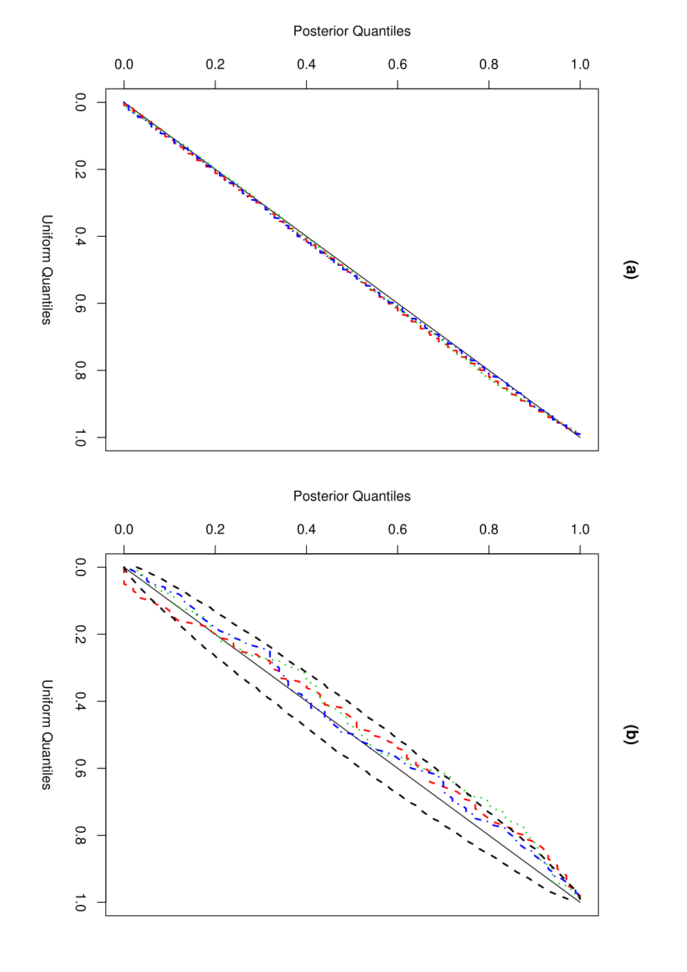
Plots of the posterior quantiles are shown in Figure 1. In both cases they are close to that expected if they were drawn from the true posterior distribution. The extra smoothness in the plot of posterior quantiles of the underlying curve is due to the larger number of quantiles obtained in this case, $100n$ as we obtain one quantile for each data point. For the posterior quantiles of $\sigma$ we are able to construct confidence intervals, as the posterior quantiles are independent. We notice that the observed quantiles generally lie within the plotted $90\%$ confidence interval. Taken together, these results suggest that negligible error is being introduced by the approximations in our method for simulating from the posterior distribution.

We now look at the accuracy of our piecewise quadratic regression model, together with the new simulation method, for curve-fitting. Firstly, in order to implement our method we need to choose the prior parameter values. As above we will use the default uninformative prior for $\sigma$. We will assume no prior knowledge of $\mathbf{D}_{0}$ and $p$, and use an empirical Bayes approach to estimate these hyper-parameters (Fearnhead, 2005, as suggested in), whereby we estimate their values from the data. We did a preliminary analysis of the data (using default choices for $\mathbf{D}_{0}$ and $p$), and then estimated $\mathbf{D}_{0}$ and $p$ from the posterior distribution of the $\beta$s and the number of changepoints. If necessary this could be repeated, with simulation from the posterior given the latest estimates for $\mathbf{D}_{0}$ and $p$, and new estimates of $\mathbf{D}_{0}$ and $p$ obtained.

For our simulation study we chose default value of $p=1/n$ and $\mathbf{D}_{0}=\mbox{diag}(10,100\times 10^{2},1000\times 40^{2})$. These are substantially different from the true values used in the simulation (see above). For simplicity we did not repeat the iterative procedure just described. The effect of these choices are discussed below.

We first quantify the accuracy of our method for analysing the same simulated data sets that were used in Section 4.1. For a given data set let $z_{t}$ denote the value of the underlying curve at time $t$ (so observations are $y_{t}=z_{t}+\sigma\epsilon_{t}$ where $\epsilon_{t}$ is a standard normal random variable). Denote by $\hat{z}_{t}$ an estimate of $z_{t}$, then we estimate the accuracy of an estimate of the curve $z_{1:n}$ by the average mean square error

For our method we use the posterior mean as our estimate of $z_{t}$. We also look at the mean point-wise coverage of $90\%$ credible (or confidence) intervals for $z_{t}$.

For comparison we estimate the underlying curve using wavelets. We implement two wavelet methods, that of Abramovich et al. (1998) implemented using the BAYES.THR function in R, and one using complex wavelets Barber and Nason (2004) implemented using the cthresh function in R. We also constructed wavelet-based confidence intervals Barber et al. (2002) using the wave.band function in R. (See http://www.stats.bris.ac.uk/$\sim$wavethresh/ for details of these functions; we used default settings for the R functions in all cases.)

Results for the simulated data described in Section 4.1 are given in Table 1. We notice that the MSE for estimates of the underlying curve is substantially smaller for our new approach than for either wavelet method. Of the two wavelet methods, the one using complex wavelets gives superior performance. The MSE of our new method halves each time $n$ is doubled, whereas the MSE of the wavelet methods decreases by a smaller proportion each time. Finally, the coverage of our 90% credible intervals are close to 90% in each case. The fact that the coverage of the intervals is less than their putative size is likely to be down to errors in estimating the hyperparameters.

The choice of default starting values for $p$ and $\mathbf{D}_{0}$, used in the iterative empirical Bayes procedure, has a small effect on the results. For example for $n=256$, repeating the analysis with default values of $p=10/n$ and $p=20/n$ increased mean square error by $0.001$ and $0.004$ respectively. Increasing the default value for $\mathbf{D}_{0}$, through scaling by a factor of 10 or 100, increased mean square error by $0.007$ and $0.011$ respectively. In these latter cases, our default value is substantially different from the truth, and we do see a non-negligible increase in mean square error. However we can avoid this by repeating the iterative procedure: for example in the last case repeating the procedure just 3 times leads to the same mean square error as reported in Table 1.

The advantage of our method over a wavelet approach for these data is not suprising as the data was simulated under the model assumed by our method. To test robustness of this method to data being simulated from an alternative model, we repeated our simulation study but with data simulated under a piecewise cubic model. For this model we set $\mathbf{D}_{0}=\mbox{diag}(1,10^{2},40^{2},d^{2})$, and considered the effect that $d$ had. Note that the expected value of the modulus of the cubic co-efficient is $d(2/\pi)^{1/2}$. For simplicity we fixed $n=256$ for all simulations that we carried out.

Results are given in Table 2, again based on 100 simulated data sets for each set of parameters. As expected, as $d$ increases, which corresponds to an increasingly non-quadratic components of the underlying curve, the performance of the new method deteriorates. This is both in terms of the coverage properties of the credible intervals, and the mean square error of estimates of the underlying curve. However for all values of $d$ we considered, the new method still substantially out-performs both wavelet methods in terms of estimating the underlying curve.

As a final comparison, we applied our new method to various test data sets from the literature, and compare our method with the published results of Denison et al. (1998) (henceforth DMS). The test data sets used are shown in Figure 2, and consist of the Heavisine, Blocks, Bumps and Doppler signals of Donoho and Johnstone (1994); and the smooth function (a) and (b) from Denison et al. (1998) (denoted DMS A amd DMS B). The method of Denison et al. (1998) uses a reversible jump MCMC to fit a piecewise cubic function, under continuity and differentiability constraints. The MCMC algorithm samples from an approximation to the posterior, based on approximating the marginal likelihood for each segment. The MCMC procedure takes up to about an order of magnitude longer to analyse the data than our approach.

We compare methods based on MSE as before. Results are given in Table 3. Our method does considerably better at estimating the curves which contain discontinuities, as our model allows for discontinuities in the underlying curve. While we do similarly or better on DMS A and DMS B, our method is substantially worse for the Bumps and Doppler data sets. This is due to errors in estimating the peaks in the Bumps data set, and the initial part of the curve in the Doppler data set. In both cases these are where the underlying curve changes most rapidly. One explanation for this is that using only quadratic polynomials, rather than cubic, makes it harder for our model to fit these parts of the curve.

The results in Denison et al. (1998) suggest that the DMS method is more accurate than using wavelets. We investigated this by calculating mean square errors for estimates obtained using the complex wavelet method implemented in cthresh. Results are given in Table 3 for the four data sets where the number of observations were an integer power of 2 (and thus it is straightforward to apply the wavelet approach). We get different results from Denison et al. (1998), with the wavelet approach out-performing the other two approaches for Bumps and Doppler, and out-performing DMS for Blocks.

Finally we look at the power of our method for detecting discontinuities in the underlying curve. Note that it is only our method that can potentially distinguish between changepoints at which the underlying curve may be either continuous or discontinuous. We focus on this feature of our method due to the application of the method we consider in Section 5.

We used as a basis the continuous curve in DMS B (see Figure 2). We then introduced a discontinuity into the curve. If we denote the underlying DMS B curve by $f(x)$ for $x\in[0,1]$, then we introduce a changepoint of size $c$ at point $x_{c}$ to produce the curve:

References

- Abramovich et al. (1998) Abramovich, F., Sapatinas, T. and Silverman, B. W. (1998). Wavelet thresholding via a Bayesian approach. Journal of the Royal Statistical Society, Series B 60, 725–749.
- Barber and Nason (2004) Barber, S. and Nason, G. P. (2004). Real nonparametric regression using complex wavelets. Journal of the Royal Statistical Society, Series B 66, 927–939.
- Barber et al. (2002) Barber, S., Nason, G. P. and Silverman, B. W. (2002). Posterior probability intervals for wavelet thresholding. Journal of the Royal Statistical Society, Series B 64, 189–205.
- Barry and Hartigan (1992) Barry, D. and Hartigan, J. A. (1992). Product partition models for change point problems. The Annals of Statistics 20, 260–279.
- Blom and Bar-Shalom (1988) Blom, H. A. P. and Bar-Shalom, Y. (1988). The interacting multiple model algorithm for systems with Markovian switching coefficients. IEEE Transactions on Automatic Control 33, 780–783.
- Chib (1996) Chib, S. (1996). Calculating posterior distributions and modal estimates in Markov mixture models. Journal of Econometrics 75, 79–98.
- Chib (1998) Chib, S. (1998). Estimation and comparison of multiple change-point models. Journal of Econometrics 86, 221–241.
- Denison et al. (1998) Denison, D. G. T., Mallick, B. K. and Smith, A. F. M. (1998). Automatic Bayesian curve fitting. Journal of the Royal Statistical Society, series B 60, 333–350.
- DiMatteo et al. (2001) DiMatteo, I., Genovese, C. R. and Kass, R. E. (2001). Bayesian curve-fitting with free-knot splines. Biometrika 88, 1055–1071.
- Dobigeon and Toumeret (2007) Dobigeon, N. and Toumeret, J. Y. (2007). Joint segmentation of wind speed and direction using a hierarchical model. Computational Statistics and Data Analysis 51, 5603–5621.
- Donoho and Johnstone (1994) Donoho, D. L. and Johnstone, I. M. (1994). Ideal spatial adaptation by wavelet shrinkage. Biometrika 81, 425–455.
- Fearnhead (2005) Fearnhead, P. (2005). Exact Bayesian curve fitting and signal segmentation. IEEE Transactions on Signal Processing 53, 2160–2166.
- Fearnhead (2006) Fearnhead, P. (2006). Exact and efficient inference for multiple changepoint problems. Statistics and Computing 16, 203–213.
- Fearnhead (2008) Fearnhead, P. (2008). Computational methods for complex stochastic systems: A review of some alternatives to MCMC. Statistics and Computing 18, 151–171.
- Fearnhead and Clifford (2003) Fearnhead, P. and Clifford, P. (2003). Online inference for hidden Markov models. Journal of the Royal Statistical Society, Series B 65, 887–899.
- Fearnhead and Liu (2007) Fearnhead, P. and Liu, Z. (2007). Online inference for multiple changepoint problems. Journal of the Royal Statistical Society Series B 69, 589–605.
- Fearnhead and Vasileiou (2009) Fearnhead, P. and Vasileiou, D. (2009). Bayesian analysis of isochores. Journal of the American Statistical Association 485, 132–141.
- Kim et al. (1998) Kim, S., Shephard, N. and Chib, S. (1998). Stochastic volatility: Likelihood inference and comparison with arch models. The Review of Economic Studies 65, 361–393.
- Lavielle and Lebarbier (2001) Lavielle, M. and Lebarbier, E. (2001). An application of MCMC methods for the multiple change-points problem. Signal Processing 81, 39–53.
- Liu and Lawrence (1999) Liu, J. S. and Lawrence, C. E. (1999). Bayesian inference on biopolymer models. Bioinformatics 15, 38–52.
- Liu et al. (1998) Liu, J. S., Chen, R. and Wong, W. H. (1998). Rejection control and sequential importance sampling. Journal of the American Statistical Society 93, 1022–1031.
- Liu (2007) Liu, Z. (2007). Direct simulation methods for multiple changepoint problems. Ph.D. thesis, Department of Mathematics and Statistics, Lancaster University.
- McVean et al. (2004) McVean, G. A. T., Myers, S. R., Hunt, S., Deloukas, P., Bentley, D. R. and Donnelly, P. (2004). The fine-scale structure of recombination rate variation in the human genome. Science 304, 581–584.
- Ó Ruanaidh and Fitzgerald (1996) Ó Ruanaidh, J. J. K. and Fitzgerald, W. J. (1996). Numerical Bayesion Methods Applied to Signal Processing. New York: Springer.
- Punskaya et al. (2002) Punskaya, E., Andrieu, C., Doucet, A. and Fitzgerald, W. J. (2002). Bayesian curve fitting using MCMC with applications to signal segmentation. IEEE Transactions on Signal Processing 50, 747–758.
- Rue and Held (2005) Rue, H. and Held, L. (2005). Gaussian Markov Random Fields: Theory and Applications. CRC Press/Chapman and Hall.
- Rue et al. (2009) Rue, H., Martino, S. and Chopin, N. (2009). Approximate Bayesian inference for latent Gaussian models by using integrated nested Laplace approximations (with discussion) . Journal of the Royal Statistical Society, Series B 71, 319–392.
- Seidou and Ouarda (2007) Seidou, O. and Ouarda, T. B. M. J. (2007). Recursion-based multiple changepoint detection in multiple linear regression and application to river streamflows. Water Resources Research 43, W07404.
- Stephens (1994) Stephens, D. A. (1994). Bayesian retrospective multiple-changepoint identification. Applied Statistics 43, 159–178.
- Tugnait (1982) Tugnait, J. K. (1982). Detection and estimation for abruptly changing systems. Automatica 18, 607–615.
- West and Harrison (1989) West, M. and Harrison, J. (1989). Bayesian forecasting and dynamic models. Springer-Verlag, New York.
- Yao (1984) Yao, Y. (1984). Estimation of a noisy discrete-time step function: Bayes and empirical Bayes approaches. The Annals of Statistics 12, 1434–1447.