Finite-size scaling tests for SU(3) lattice gauge theory with color sextet fermions
Abstract
The observed slow running of the gauge coupling in SU(3) lattice gauge theory with two flavors of color sextet fermions naturally suggests it is a theory with one relevant coupling, the fermion mass, and that at zero mass correlation functions decay algebraically. I perform a finite-size scaling study on simulation data at two values of the bare gauge coupling with this assumption and observe a common exponent for the scaling of the correlation length with the fermion mass, . An analysis of the scaling of valence Dirac eigenvalues at one of these bare couplings produces a similar number.
I Introduction and theoretical background
Recently, many researchers [1, 2, 3, 4, 5, 6, 7, 8, 9, 10, 11, 12, 13, 14, 15, 16, 17, 18, 19] have begun to use lattice methods to study field theories which might be candidates for strongly coupled beyond - Standard Model new physics [23]. These models typically involve gauge fields and a large number of fermion degrees of freedom, either many flavors of fundamental representation fermions (where the discussion goes back to Refs. [24, 25]) or a smaller number of flavors of higher-dimensional representation fermions (strongly emphasized by Refs. [26, 27, 28]).
The usual description of renormalization for a gauge theory coupled to massless fermions classifies the possibilities for its behavior according to how the gauge coupling flows under rescaling to the infrared: it could flow to strong coupling in the case of a confining theory, or to zero, for a trivial theory, or to a fixed point at some nonzero value, . The latter case is referred to as an infrared-attractive fixed point (IRFP) theory. This is a phase with no confinement, no chiral symmetry breaking, and algebraic decay of correlation functions. Evidence has been presented that several such theories exist: gauge theory with flavors of fundamental fermions [4, 14], gauge theory with flavors of sextet fermions (the subject of this paper) [5] and gauge theory with flavors of adjoint fermions[15].
While for confining theories the gauge coupling is relevant (the Gaussian fixed point is unstable), that is not the case for IRFP theories. The distance of the bare gauge coupling from its fixed point value is an irrelevant coupling. The critical surface encompasses a wide range of values of bare gauge couplings. The fermion mass is a relevant coupling of an IRFP theory, since it must be fine-tuned at the UV scale to reach the critical surface (i.e. ). The situation is completely equivalent to that of an order-disorder transition in a magnetic system. The only difference is that the relevant direction is parameterized by the quark mass , rather than by the reduced temperature of the magnet. (A closer analogy is to a system which has been fine tuned to its Curie point and then placed in an external magnetic field. The external field breaks the underlying global symmetry just as a quark mass explicitly breaks chiral symmetry.) [29]
The framework to describe the physics of these systems is standard. It involves a set of scaling operators which evolve independently and multiplicatively and whose renormalization group (RG) equations have linear zeroes; the RG equation for the change in the th coupling, under a scale change by a factor , linearized around its fixed-point value , is
| (1) |
The mass is the relevant coupling and its exponent will be labeled . Tuning the mass to zero causes the correlation length to diverge algebraically,
| (2) |
The exponent is related to the evolution of the condensate in beyond-Standard Model phenomenology. Under a change of scale from to , the condensate runs as
| (3) |
where is its scaling dimension. ( where is its anomalous dimension). Because the combination is an RG invariant, .
Thus is an interesting object[30]. The subject of this paper is a calculation of for gauge fields coupled to flavors of fermions in the sextet (color symmetric) representation.
Most recent lattice work on candidate theories is devoted to answering the question of whether or not the gauge coupling runs to a fixed point. The analysis in this paper simply assumes that the gauge coupling runs very slowly. What happens in that case can be seen from an elaboration of Eq. 3. Suppose that we have a correlation function measured on a momentum scale which is large compared to other possible scales in the theory. Then, textbooks tell us that a generic correlation function (with engineering dimension and associated anomalous dimension ) scales as
| (4) |
When the integral is dominated by scales where the coupling is given by its fixed point value, then where . The correlator has power law behavior. (This behavior is modified at short distances by non-scaling terms in the action.)
If we have a real fixed point, then the critical exponents (in this case, ) will not depend on the value of the bare coupling. However, imagine that we do not have a fixed point. Then the integral in Eq. 4 will depend on . But if the change in the coupling over the range of the integral is small, will remain unchanged, and one will again observe a power law behavior for correlators. Of course, the value of the exponent would change as the bare coupling were varied. Whether one is seeing a real exponent (a constant ) or an effective one (that is, one is mapping out ) can be tested by determining for several values of the bare gauge coupling.
This discussion would be redundant if we knew from other sources whether the theory was in the IRFP phase or not. It is necessary to make it because this part of the story is not complete. It is quite clear that, in my system’s weak coupling phase, observables (correlation lengths) depend quite strongly on the quark mass and only weakly on the gauge coupling. The correlation length saturates at a value proportional to the size of the system as the quark mass is tuned to zero.
And in the weak coupling phase, the running coupling does run slowly. Last year Svetitsky, Shamir and I [5] presented evidence that sextet fermions and gauge fields had an IRFP. Those simulations were done with a different bare action than the one used here. We are repeating and extending our calculation of the running coupling using the present bare action. That analysis is at present incomplete [31]. At this point in time, we know that throughout the weak coupling phase the running coupling (defined through the Schrodinger Functional (SF) scheme) runs more slowly than two-loop perturbation theory predicts. This itself is slow running compared to the familiar case of fundamental representation QCD. That this should be so is obvious from the beta function, but the numerical values are worth mentioning. At the two bare couplings where I will claim a measurement of , the SF coupling (measured on volumes) is about at and about 3.4 at . (Parameter sets will be given below.) The change of in a scale factor of 2 from integrating the two-loop perturbative beta function is about -0.2 and -0.3 respectively – about ten per cent. This justifies treating the gauge coupling as if it were not running and looking for deviations. For the more familiar case of gauge group and fundamental fermions, the change would be -0.8 and -2.0 at these couplings. (And in this case the observed coupling runs faster than the perturbative result.[32].)
Looking ahead to my answer, I claim that at the two values of the bare coupling where I measured it.
I will investigate three different ways to measure .The successful ones employ finite size scaling arguments for the response of observables to the simulation volume.
The first way uses the correlation length directly. When it grows to be the size of the simulation volume, Eq. 2 breaks down. Finite size scaling arguments allow us to use the breakdown to determine the exponent. This test is done at two values of the bare coupling.
The two other tests involve working with extensive quantities. As is tuned to zero, the singular part of the free energy scales as
| (5) |
where is the system’s dimensionality (here ), and the prefactor is just (the correlation length provides the appropriate dimensional factor). and are non-universal constants and is the biggest non-leading exponent. This is most likely the exponent of the gauge coupling, , which can be determined from the beta function as measured in (for example) Schrodinger functional simulations at . It is probably small; in Ref. [29], Hasenfratz and I estimated that it was close to zero in this and related theories.
So the condensate, , scales with as
| (6) |
where . This is exactly like the relation of the specific heat exponent to the correlation length exponent at a conventional paramagnetic-ferromagnetic critical point.
Working with the condensate has the problem that the particular lattice fermions used in this simulation, Wilson-type fermions, explicitly break chiral symmetry in the action. This introduces an additive shift to the condensate. So I will use partial quenching: I will take configurations generated with lattice fermions which do not have exact chiral symmetry, and measure the Dirac spectrum using valence quarks which are an implementation of lattice fermions with exact chiral symmetry (overlap fermions). One can question whether the valence fermion sees a faithful realization of what is happening in the equilibrium distribution of real dynamical variables. In usual (low- fundamental QCD) this is believed to be the case. I think that for a first study, what I am going to do is adequate. (It would of course be better to do simulations with chiral dynamical fermions, as was done by the authors of Ref. [9], but they are presently too expensive for simulations at large volume.)
The condensate has UV-sensitive pieces [33], where and . This masks the non-analytic behavior. This is quite similar to the situation in finite temperature QCD, precisely at , where[34]
| (7) |
An IRFP theory is different from QCD in that there are no Goldstone bosons (which contribute their own non-analytic piece to the condensate, below ). It is also different from QCD in that while in QCD, Eq. 7 applies only at , in an IRFP theory Eq. 7 gives the behavior of the condensate throughout the basin of attraction of the IRFP. Unfortunately, for my data set, the UV terms dominate .
A better way to attack through the condensate involves the Banks-Casher relation[35] between the condensate and the density of eigenvalues of the Dirac operator . At nonzero mass it is
| (8) |
If the massless theory is conformal, and the condensate for small mass, then also scales as . A finite-size scaling argument[36] relates the scaling for the density to the scaling of the value of individual eigenvalues. If we consider the average value of the th eigenvalue of the Dirac operator in a box of volume , and if , then we expect
| (9) |
where the exponent is
| (10) |
For the case of an IRFP theory, is equal to , the leading exponent.
(To derive this, note means that eigenvalues are uniformly distributed in an dimensional space of volume ,
| (11) |
so an eigenvalue scales as . Now suppose we are in physical dimensions; in a box of volume , there are modes, from which Eq. 10 is obtained.)
One example of this formula is free field theory: and . Another is the case of chiral symmetry breaking encoded in the usual formulas of its Random Matrix Theory analog: so a constant, and . This is , which is equivalent to the usual statement that the eigenvalue spectrum depends on the dimensionless product .
For the case of a system which exhibits chiral symmetry breaking, there is a tight theoretical description of the behavior of the lowest eigenvalues of the Dirac operator, which allows one to relate delicate features of the spectrum to the low energy constants of the theory (the condensate, the pseudoscalar decay constant, and possibly others). This description is based on Random Matrix Theory (RMT). However, if a system is in a chirally-restored phase, there are no longer RMT predictions to compare results against. Previous work shows that our target theory has a weak-coupling phase which is chirally-restored. The restoration of chiral symmetry is observed through regularities in the spectrum of screening masses as well as the behavior of the pseudoscalar decay constant as a function of quark mass. Therefore, the analysis reported here only uses the simplest property of the eigenvalues, namely their scaling with system size.
The paper proceeds as follows. In Sec. II I describe details of the simulations. In Sec. III I compute the correlation length exponent using finite size scaling. Next, in Sec. IV I examine the mass dependence of the chiral condensate, and finally in Sec. V I perform a scaling test for eigenvalues of the valence Dirac operator. I conclude with a discussion of my results.
In an earlier preprint [38] I tried to do several of the analyses I report on, in this paper. In Ref. [11] we observed that in the deconfined phase of sextet QCD, the Polyakov loop ordered in one of the negative real directions, roughly along one of the complex elements of , (, ). I believed that was the general situation for this theory and all the simulations were done in those vacua. After that paper appeared, detailed studies of the phase structure (at smaller volumes) by Machtey and Svetitsky [37] showed that the true vacuum of the deconfined phase is in fact the one in which the Polyakov loop is real and positive. All the results of Ref. [38] only apply to metastable vacua. Their conclusion renders it too uninteresting to publish.
II Numerical techniques and background
I performed simulations on a system with gauge fields and two flavors of dynamical fermions in the symmetric (sextet) representation of the color gauge group. The lattice action is defined by the single-plaquette gauge action and a Wilson fermion action with added clover term [39]. The fermion action employs the differentiable hypercubic smeared link of Ref. [40], from which the symmetric-representation gauge connection for the fermion operator is constructed. No tadpole-improvement is used and the clover coefficient is set to its tree-level value. The smearing parameters for the links are the same as in Ref. [40], , , . The bare parameters which are inputs to the simulation are the gauge coupling and the fermion hopping parameter . The integration is done with one additional heavy pseudo-fermion field as suggested by Hasenbusch [41], multiple time scales [42], and a second-order Omelyan integrator [43].
The routines for simulating sextet-representation fermions were developed with (and mostly by) B. Svetitsky and Y. Shamir. The dynamical fermion algorithm was adapted from a program written by A. Hasenfratz, R. Hoffmann and S. Schaefer[44] All computer code is based on the publicly available package of the MILC collaboration [45].
Simulation volumes range up to sites, and typical data sets range from a few hundred to a thousand trajectories. I recorded lattices every five trajectories (of unit simulation time trajectory length) and collected 40 lattices per parameter set for the calculation of spectral observables and overlap eigenvalues.
Correlation lengths are taken to be inverses of screening masses, from correlators of operators at different separations measured along one of the spatial directions of the lattice. The trick of combining periodic and anti-periodic boundary conditions for valence quarks [46, 47, 48, 49] is used in these measurements.
Throughout this work, instead of quoting , I will use the the Axial Ward Identity (AWI) quark mass, defined through
| (12) |
where , , and is any source. The derivative is taken to be the naive difference operator (). For I used a Coulomb gauge-fixed Gaussian source.
Machtey and Svetitsky [37] have performed careful studies of the phase structure of this theory and have shown that that the true vacuum (in the deconfined phase) is the one in which the expectation value of the Polyakov loop is real and positive. All simulations reported here were done in this vacuum.
The valence Dirac operator whose eigenvalues are used in Sec. V is the overlap operator [50, 51]. Details of the particular implementation of the action are described in Refs. [52, 53, 54, 55, 56]. The only new ingredient is the application to symmetric-representation fermions, using the same combination of hypercubic link and projection into the fermionic representation as for the dynamical fermions. Eigenvalues of the squared Hermitian Dirac operator are computed using the “Primme” package of McCombs and Stathopoulos[57] and split apart in the usual way. Eigenvalues are quoted after stereographic projection.
There is a potential problem with this analysis involving the index theorem, relating the winding number of the gauge field to the number of Dirac fermion zero modes,
| (13) |
is the Dynkin index of the representation , 1/2 for fundamental representation fermions, for two-index symmetric representation fermions in the color group , and so on. Thus we expect to see multiples of 5 zero modes for sextet overlap fermions in our case.
However, ten years ago Heller, Edwards, and Narayanan discovered[58] that the index theorem applied to adjoint overlap fermions in background gauge configurations failed: while , they saw configurations with zero modes which were not multiples of four. More recently, similar results were reported by Garcia Perez, Gonzalez-Arroyo and Sastre[59]. In simulations where the bare gauge coupling is large, I have seen configurations whose zero mode content was a not a multiple of 5.
Fortunately, the authors of Ref. [60] have studied the index theorem for sextet representation fermions in quenched background gauge field configurations and shown that in the continuum limit only configurations with multiples of five zero modes are found. The “fractional states” are apparently just a particular failure of the overlap action to capture topology when the gauge configuration is rough.
This is not a problem for this project. The gauge configurations at the parameter value used to compute eigenvalues () were smooth enough that all of the lattices I collected had . I performed some trial simulations at a lower of 4.8 and also saw only . However, for these rougher configurations the cost of the overlap operator went up by about a factor of four, and it did not seem like a good use of computer time to continue running there.
A map of the simulation region is shown in Fig. 1. It is qualitatively similar to what we found with another bare action [11]. The line is the location in bare parameter space where the AWI quark mass vanishes, . The crosses show the location of the deconfinement phase transition. To the left of this line, the system is confined and seems to be chirally broken. However, this region is little explored. It is unknown how (or if) the deconfinement line attaches to the line. To the right of the line, the system is deconfined on all observed volumes and spectroscopy shows parity doubling. This plus the smallness of the pseudoscalar decay constant leads me to conclude that the system is in a chirally restored state throughout that phase. All data used in this study comes from the weak coupling phase.
Table 1 lists all simulation points use in this study. Since I will report results in terms of the AWI quark mass, I include it in the table. When there are several volumes, the quoted mass is from the smallest volume. However, generally the volume dependence of the quark mass is small ( a few digits in the least significant figure). In the analysis, data from any particular volume is plotted and used at its measured quark mass in that volume. As falls, the available parameter space in the deconfined phase shrinks to a smaller and smaller range of quark masses.

| volumes | |||
| 4.20 | 0.1370 | 0.110 | |
| 4.40 | 0.1335 | 0.106 | |
| 4.40 | 0.1345 | 0.052 | |
| 4.60 | 0.1300 | 0.165 | , |
| 4.60 | 0.1320 | 0.065 | , |
| 4.60 | 0.1325 | 0.027 | |
| 4.80 | 0.1230 | 0.412 | , , |
| 4.80 | 0.1250 | 0.300 | , , |
| 4.80 | 0.1260 | 0.233 | |
| 4.80 | 0.1270 | 0.209 | , , |
| 4.80 | 0.1285 | 0.146 | , , |
| 4.80 | 0.1290 | 0.104 | , , |
| 4.80 | 0.1300 | 0.086 | , , , |
| 5.20 | 0.1100 | 0.940 | , |
| 5.20 | 0.1150 | 0.630 | , |
| 5.20 | 0.1220 | 0.310 | , |
| 5.20 | 0.1235 | 0.220 | |
| 5.20 | 0.1250 | 0.195 | , , |
| 5.20 | 0.1270 | 0.096 | |
| 5.20 | 0.1285 | 0.066 | , , , , , , |
| 5.20 | 0.1290 | 0.047 | , , |
III Finite-size scaling
I begin this section with several pictures of spectroscopy to set the stage. Fig. 2 are plots of screening masses at on and volumes. These two panels show that in the weak coupling phase the excitation spectrum is parity doubled and that the pseudoscalar decay constant becomes small as the quark mass vanishes.

Throughout the weak coupling phase, masses depend strongly on the quark mass and weakly on the bare gauge coupling. Fig. 3 illustrates this feature for the correlation length, defined as the inverse of the pseudoscalar screening mass, showing volumes on the left and volumes on the right. Different plotting symbols correspond to different values.

Finally, I combine data from many volumes at one gauge coupling, , in Fig. 4. The saturation of the correlation length at a scale proportional to the temporal length of the lattice is apparent. Superficially, this is just the Matsubara cutoff expected from the fermions’ antiperiodic temporal boundary conditions.

The relation between correlation length and quark mass given by Eq. 2 is only expected to hold when the system size is much larger than . When the correlation length measured in a system of size (call it ) becomes comparable to , saturates at even as vanishes. However, if the only large length scales in the problem are and , then overall factors of length can only involve and . For the correlation length itself, this argument says that
| (14) |
where is some unknown function of . A somewhat more useful version of this relation can be written by using Eq. 2 to say
| (15) |
Then one can plot vs for many ’s, vary , and look for the appearance of a smooth curve. The data from different ’s will march across the x axis at different rates.
A good data set to use is the one of Fig. 4, . These are screening masses, so I will take regardless of the value of . A scan of Eq. 15 is shown in Fig. 5. Already one can see that a choice of pulls all the data from Fig. 4 onto a single curve.

To turn this observation into a number with an uncertainty is a bit awkward. We are not doing a fit, because the function of Eq. 15 is unknown. Instead I will do the analysis in two different ways:
First [61] take the full range of values of and slice it into a set of bins. In the th bin, define
| (16) |
and
| (17) |
Then define a goodness-of-fit parameter as
| (18) |
Minimize this function with respect to and fold the whole procedure into a jackknife over all the different mass- combinations to get an uncertainty. The division by mimics the eye’s attempt to minimize the fractional spread of the points about their average. Notice that bins with only a single entry do not contribute to . Binning the data introduces the possibility of a dependency on the number of bins. I assign an error by jackknifing the data set. In practice, if there are too many bins, there are seldom bins with more than one point, and the jackknife error becomes large.
A second approach follows the method of Ref. [62]. The idea is to use each data set (each different value) to estimate and to find the which pulls the other sets onto it. This is done inclusively; all data sets take a turn at being the fiducial. The quantity to minimize is
| (19) |
The interpretation of this long formula is that data set is used to estimate the scaling function . This is done by interpolation, either by polynomials or rational functions, using the recorded values of . The label “over” indicates that the sum only includes data from set whose values, , overlap the range of ’s of set . The overall factor of counts the total number of points and guards against recording a zero value of if there are no overlap. (Bhattacharjee and Seno actually consider powers other than two inside the sum.) is minimized by the optimal . This method has an advantage over the first one that one does not need to bin the data, and a disadvantage that the interpolation algorithm has to be robust. This can be a problem for extreme values of . The number varies as is tuned. This could potentially make discontinuous.
The two methods produce similar results. At there are 23 separate data points (values of and ), with ranging from about 0.08 to 0.16. Asking for 5 bins gives (on average) 4 useful bins and . Asking for 6 bins gives 5 useful bins and . Asking for 8 bins produces on average 5 useful bins and . With the second method, from a single-elimination jackknife over the data set.
Bhattacharjee and Seno advocate taling an error from an approximation to the second derivative of P,
| (20) |
With this produces .
At the situation is similar, but noisier. I again have four ’s, from , , and volumes (, 8, 12, 16 respectively) and a total of 21 mass and size combinations. The data is noisier than the data set. Fig. 6 shows the data before and after collapse to a line. A five-bin single jackknife fit gives while the second method gives 1.41(26). The approximate second derivative gives . A conservative summary of values and uncertainties is at and 1.4(2) at .
In this analysis, I made a particular choice of a geometry and a method of defining a correlation function (screening masses, sensitive to the length of the antiperiodic boundary condition in the temporal direction). I do not believe that it is better than alternative methods one could try (for example, taking volumes and varying ). People interested in finite size scaling tests should try other geometries.
In the statistical mechanics finite size scaling literature it is common to perform finite size scaling analyses on susceptibilities. I have experimented with this, but probably not extensively enough. Mocking up susceptibilities by integrating over correlation functions () has not produced interesting peaks, because the correlators – and their integrals – are dominated by short distance effects. This deserves more study.

IV The condensate directly from the overlap operator
In this section and the next one, I only have data at . I ran at one value, . This corresponds to a small AWI mass. As I remarked, it was quite expensive to evaluate the overlap operator at stronger coupling.
The condensate is measured in the usual way, with a vector of Gaussian random numbers defined on every site of the lattice, , through an average over the random vectors,
| (21) |
and as usual for the overlap operator, is the subtracted, shifted Dirac operator . I accelerated the inversion by deflating with the eight smallest eigenmodes of . This is all quite standard [52]. Even a small data set (twenty lattices, twelve random vectors per lattice) produces a nice signal (Fig. 7a), which is almost completely linear in the quark mass. This demonstrates rather dramatically that the gauge field configurations at one point in the weak coupling phase do not allow chiral valence quarks to form a condensate. The linear behavior is just the UV-dominated (proportional to ) term in the expected expansion. I tried to remove it using a variation on a trick from Ref. [63]: Compute for each random number, for many masses simultaneously by using a multi-mass sparse matrix inversion algorithm. Then pick a mass as a fiducial and compute the difference random number by random number. Finally, form the average over random seeds. The high correlations in the values of the condensate for different masses are removed from the error budget in . I took nine masses ranging from to 0.25 and used . The result is shown in Fig. 7b.
Unfortunately, a fit of to a power, , produces a noisy result that . The exponent is unstable against the set of masses included in the fit. This is most likely (and one could not argue that it is not) just the nonleading UV term (). Thus this attempt fails. Something else is required, which is insensitive to the UV part of the condensate. That follows in the next Section.

V Finite size scaling of Dirac eigenvalues
To test the scaling law of Eq. 9 I generated ensembles of lattices at one set of bare parameters, and , and a number of simulation volumes, and computed the lowest eight eigenvalues of the massless overlap Dirac operator on them. The bare parameter set was chosen to have a light valence quark mass and to be within the weak coupling phase. All of the configurations collected at this parameter value have zero topological charge. To see scaling, it is necessary to preserve the geometry of the simulation volume (to compare, for example lattices at different ’s). My primary data set is lattices with , 10, 12, and 16. The resulting eigenvalue spectrum is shown in Fig. 8. By eye, it seems to show power law behavior.

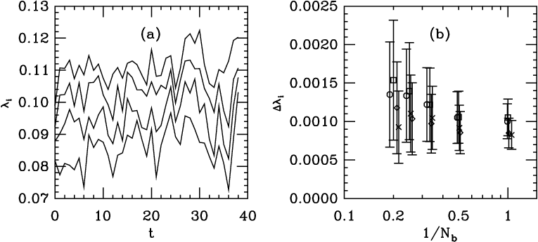
Fig 9 illustrates the quality of the data. The left panel shows simulation time histories of the lowest four eigenvalues of the data set. Each measurement is separated by five HMC trajectories. The right panel shows the error on the average computed by blocking successive measurements together. The lowest eigenvalue is clearly the noisiest, but the autocorrelation time does not seem to be too large: I bin two successive lattices ( or HMC units) together before averaging.
Now I wish to extract an exponent from Fig. 8. For theoretical input, all we have is Eq. 9, the finite-size scaling formula. One does not know a priori if it applies to all the eigenvalues, only to the lowest eigenvalues, or if there is some minimum volume for which it applies. I will just proceed empirically: I will look at fits to individual eigenvalues, then groups of them. I will fit all the data sets or drop the smallest volume and fit only the larger ones.
I begin by fitting individual eigenvalues (lowest, second, and so on) to a power law, . I choose to fit to all four volumes, or the largest three. The individual data points in each fit are uncorrelated, of course. Fits and chi-squareds are shown in Table 2. Examples of fits are shown in Figs. 10 and 11.


I also fit groups of eigenvalues, using for eigenvalues. Now the data are correlated. I look at the quality of fits from uncorrelated fits, and then repeat by taking bootstrap averages of the data. The behavior is quite similar to the fits to individual eigenvalues. Some examples (with bootstrap errors) on the average, chi-squared from uncorrelated fits:
- •
Fit the lowest 4 eigenvalues and biggest 3 volumes: ,
- •
Fit the lowest 4 eigenvalues 4 volumes: ,
- •
Fit all 8 eigenvalues and biggest 3 volumes: ,
- •
Fit all 8 eigenvalues and 4 volumes: ,
Examples of these fits are shown in Fig. 12.
| 3 volumes | 4 volumes | |||
|---|---|---|---|---|
| mode | ||||
| 1 | 1.64(4) | 3.0 | 1.60(3) | 5.2 |
| 2 | 1.64(4) | 4.3 | 1.59(3) | 8.0 |
| 3 | 1.61(3) | 11.4 | 1.56(2) | 16.5 |
| 4 | 1.58(3) | 18.7 | 1.52(2) | 26.2 |
| 5 | 1.53(2) | 13.7 | 1.49(2) | 19.2 |
| 6 | 1.51(3) | 10.0 | 1.47(2) | 17.0 |
| 7 | 1.48(2) | 11.6 | 1.45(2) | 17.0 |
| 8 | 1.45(2) | 8.4 | 1.43(2) | 11.4 |
The numerical value of the eigenvalues depends on the geometry of the lattice, but the scaling exponent does not seem to do so. I have data from and lattices. Fitting them as was done for the other data sets produces a similar exponent (similar results for individual or multiple eigenmodes, from a fit to the lowest four modes, ). See Fig. 13 for an example. With two volumes, of course, one can assume any scaling law that one wants. Nevertheless forcing a power law yields an exponent which is similar to that from volumes.

At the end of this analysis I have many numbers, all rather similar but none really identical. What is missing from this section is some way of estimating the correction to scaling due to cutoff effects. In RMT, the larger eigenmodes are the ones which are most affected by non-infrared physics. Kovacs [64] has pointed out that in distributions like , the lowest eigenvalue has the broadest distribution and is most susceptible to finite statistics. Theoretical guidance is needed. Nevertheless, the observed exponents seem to be in quite good accord with the value of observed in Sec. III, at .
VI Discussion
The lattice-regulated system of flavors of sextet fermions coupled to gauge fields has a weak coupling phase which is chirally restored. Within that phase, hadronic correlation lengths (masses) show a weak dependence on the value of the bare gauge coupling. At one observation point in this phase, I find that the valence quark condensate vanishes as its (valence) mass is taken to zero.
Motivated by the realization that slow running is very similar to no running (recall Eq. 4), I analyzed the correlation length in the weak coupling phase as if its massless limit were critical, with the size of the relevant perturbation given by the AWI quark mass. I observed the collapse of correlation length data from many lattice sizes onto a common scaling curve. I did this at two bare parameter values. The observed exponent was identical within rather large errors. Roughly the same exponent governs the scaling of the values of low lying valence overlap Dirac eigenvalues at one of the couplings. My data cannot show whether the theory truly has only one relevant operator (with coupling proportional to the quark mass) and the gauge coupling is irrelevant, or if the gauge coupling is also running very slowly. This remains an open question.
My analysis assumes that the correlation length would diverge at zero AWI quark mass in the infinite volume limit. The exponent is not unity, the value expected for a free field theory. The system thus has interacting dynamics.
Recall that . The perturbative expectation is . Inserting the Schrodinger functional coupling quoted in the Introduction for these bare coupling values, perturbation theory predicts and -0.41 at the two couplings. This is a bit smaller than what I measure. (Of course, one could argue about the choice of a coupling in a perturbative formula.)
Ryttov and Sannino [65] have a supersymmetric QCD - inspired beta function for gauge theories with higher dimensional representations of fermions. The anomalous dimension is predicted to be
| (22) |
for the case studied here. My result disagrees with their prediction.
This research leaves some obvious open questions. First, I have nothing to say about the strong coupling end of the weak coupling phase.
Next, it is unknown if this theory has an IRFP or merely runs very slowly. Once that is known, results from this paper can be used for physics analyses. Even with the present statistical significance of my result, there are some rather definite conclusions which can be drawn once the answer to this question is known.
If this theory does not have an IRFP, can be used to run the condensate down according to Eq. 3. seems to be a bit larger than perturbation theory would give. Of course, collecting more points will give a nonperturbative determination of as a function (if any) of .
If this theory is in fact an IRFP theory, my result indicates that it might not be a very spectacular IRFP theory, and it may not be phenomenologically interesting. This is because the exponent is small. Unitarity bounds for conformal field theories[66, 67] constrain the scaling dimension of the leading scalar operator (which I am inferring will be the condensate, or at least what the fermions mass couples to) to lie in the range . My is safely in that range. But in “unparticle” extensions of the Standard Model, new physics (NP) at scale influences Standard Model (SM) physics at scale through terms in an effective Lagrangian of the form
| (23) |
where the dimension of the new physics operator is and the ’s are operators in the two sectors. In the literature, is generally desired to be as small as possible to enhance its effective coupling (the prefactor of the operator product). Luty and Okui [68], for example, discuss models with in the range 1-2. There is also an extensive literature relating the lower end of the conformal window to large , with perhaps having a connection with physics which closes the window. (See Refs. [69, 70, 71, 72, 73, 74].) For sextet QCD, is almost certainly close to the top of the conformal window, and is almost certainly confined, so if is conformal with there is not much of a story to be told.
There are two other cases where has been measured. The first is gauge theory with fundamental representation flavors. Here, close to the top of the conformal window for its representation class, Hasenfratz [75] has found . It is not surprising that is greater than 1 for sextet QCD since is expected to increase with increasing distance from the top of the conformal window. The authors of Ref. [22] report a determination of for gauge fields and adjoint fermions. They also find it is small.
Understanding strongly-coupled beyond-Standard Model physics requires studying many theories and computing the anomalous dimensions for enough of them to be able to understand systematic trends. Finite size scaling studies are a useful way to do this.
Acknowledgements.
I thank P. Damgaard, C. DeTar, A. Hasenfratz, A. Jackson, T. G. Kovacs, D. Nógrádi, S. Pigolotti, K. Rummukainen, Y. Shamir, and B. Svetitsky for discussions. I am grateful for the hospitality of the Niels Bohr International Academy during the time I carried out this research. This work was supported in part by the US Department of Energy.References
- [1] P. H. Damgaard, U. M. Heller, A. Krasnitz and P. Olesen, Phys. Lett. B 400, 169 (1997) [arXiv:hep-lat/9701008].
- [2] U. M. Heller, Nucl. Phys. Proc. Suppl. 63, 248 (1998) [arXiv:hep-lat/9709159].
- [3] S. Catterall and F. Sannino, Phys. Rev. D 76, 034504 (2007) [arXiv:0705.1664 [hep-lat]].
- [4] T. Appelquist, G. T. Fleming and E. T. Neil, Phys. Rev. Lett. 100, 171607 (2008) [arXiv:0712.0609 [hep-ph]].
- [5] Y. Shamir, B. Svetitsky and T. DeGrand, Phys. Rev. D 78, 031502 (2008) [arXiv:0803.1707 [hep-lat]].
- [6] A. Deuzeman, M. P. Lombardo and E. Pallante, Phys. Lett. B 670, 41 (2008) [arXiv:0804.2905 [hep-lat]].
- [7] L. Del Debbio, A. Patella and C. Pica, arXiv:0805.2058 [hep-lat].
- [8] S. Catterall, J. Giedt, F. Sannino and J. Schneible, JHEP 0811, 009 (2008) [arXiv:0807.0792 [hep-lat]].
- [9] Z. Fodor, K. Holland, J. Kuti, D. Nogradi and C. Schroeder, arXiv:0809.4888 [hep-lat].
- [10] L. Del Debbio, A. Patella and C. Pica, arXiv:0812.0570 [hep-lat].
- [11] T. DeGrand, Y. Shamir and B. Svetitsky, Phys. Rev. D 79, 034501 (2009) [arXiv:0812.1427 [hep-lat]].
- [12] A. J. Hietanen, J. Rantaharju, K. Rummukainen and K. Tuominen, JHEP 0905, 025 (2009) [arXiv:0812.1467 [hep-lat]].
- [13] G. T. Fleming, PoS LATTICE2008, 021 (2008) [arXiv:0812.2035 [hep-lat]].
- [14] T. Appelquist, G. T. Fleming and E. T. Neil, Phys. Rev. D 79, 076010 (2009) [arXiv:0901.3766 [hep-ph]].
- [15] A. J. Hietanen, K. Rummukainen and K. Tuominen, arXiv:0904.0864 [hep-lat].
- [16] A. Deuzeman, M. P. Lombardo and E. Pallante, arXiv:0904.4662 [hep-ph].
- [17] Z. Fodor, K. Holland, J. Kuti, D. Nogradi and C. Schroeder, arXiv:0907.4562 [hep-lat].
- [18] L. Del Debbio, B. Lucini, A. Patella, C. Pica and A. Rago, arXiv:0907.3896 [hep-lat].
- [19] C. Pica, L. Del Debbio, B. Lucini, A. Patella and A. Rago, arXiv:0909.3178 [hep-lat].
- [20] D. K. Sinclair and J. B. Kogut, arXiv:0909.2019 [hep-lat].
- [21] T. Appelquist et al., arXiv:0910.2224 [hep-ph].
- [22] F. Bursa, L. Del Debbio, L. Keegan, C. Pica and T. Pickup, arXiv:0910.2562 [hep-ph].
- [23] For a review of the phenomenology, see C. T. Hill and E. H. Simmons, Phys. Rept. 381, 235 (2003) [Erratum-ibid. 390, 553 (2004)] [arXiv:hep-ph/0203079].
- [24] W. E. Caswell, Phys. Rev. Lett. 33, 244 (1974).
- [25] T. Banks and A. Zaks, Nucl. Phys. B 196, 189 (1982).
- [26] F. Sannino and K. Tuominen, Phys. Rev. D 71, 051901 (2005) [arXiv:hep-ph/0405209].
- [27] D. D. Dietrich and F. Sannino, Phys. Rev. D 75, 085018 (2007) [arXiv:hep-ph/0611341].
- [28] T. A. Ryttov and F. Sannino, Phys. Rev. D 76, 105004 (2007) [arXiv:0707.3166 [hep-th]].
- [29] For a review, see T. DeGrand and A. Hasenfratz, Phys. Rev. D 80, 034506 (2009) [arXiv:0906.1976 [hep-lat]].
- [30] Compare the earlier discussion by M. A. Luty, JHEP 0904, 050 (2009) [arXiv:0806.1235 [hep-ph]].
- [31] DeGrand, Shamir and Svetitsky, work in progress; B. Svetitsky, lecture given at Universe in a Box: LHC, Cosmology and Lattice Field Theory, Leiden, August 2009 (unpublished).
- [32] M. Della Morte, R. Frezzotti, J. Heitger, J. Rolf, R. Sommer and U. Wolff [ALPHA Collaboration], Nucl. Phys. B 713, 378 (2005) [arXiv:hep-lat/0411025].
- [33] H. Leutwyler and A. V. Smilga, Phys. Rev. D 46, 5607 (1992).
- [34] F. Karsch [RBC-Bielefeld collaboration], Nucl. Phys. A 820, 99C (2009) [arXiv:0810.3078 [hep-lat]].
- [35] T. Banks and A. Casher, Nucl. Phys. B 169, 103 (1980).
- [36] G. Akemann, P. H. Damgaard, U. Magnea and S. M. Nishigaki, Nucl. Phys. B 519, 682 (1998) [arXiv:hep-th/9712006].
- [37] O. Machtey and B. Svetitsky, private communication.
- [38] T. DeGrand, arXiv:0906.4543 [hep-lat].
- [39] B. Sheikholeslami and R. Wohlert, Nucl. Phys. B 259, 572 (1985).
- [40] A. Hasenfratz, R. Hoffmann and S. Schaefer, JHEP 0705, 029 (2007) [arXiv:hep-lat/0702028].
- [41] M. Hasenbusch, Phys. Lett. B 519, 177 (2001) [arXiv:hep-lat/0107019].
- [42] C. Urbach, K. Jansen, A. Shindler and U. Wenger, Comput. Phys. Commun. 174, 87 (2006) [arXiv:hep-lat/0506011].
- [43] T. Takaishi and P. de Forcrand, Phys. Rev. E 73, 036706 (2006) [arXiv:hep-lat/0505020].
- [44] A. Hasenfratz, R. Hoffmann and S. Schaefer, Phys. Rev. D 78, 054511 (2008) [arXiv:0806.4586 [hep-lat]].
- [45] http://www.physics.utah.edu/%7Edetar/milc/
- [46] T. Blum et al. [RBC Collaboration], Phys. Rev. D 68, 114506 (2003) [arXiv:hep-lat/0110075].
- [47] Y. Aoki et al., Phys. Rev. D 73, 094507 (2006) [arXiv:hep-lat/0508011].
- [48] C. Allton et al. [RBC and UKQCD Collaborations], Phys. Rev. D 76, 014504 (2007) [arXiv:hep-lat/0701013].
- [49] C. A. Aubin, J. Laiho, and R. S. Van de Water, arXiv:0710.1121 [hep-lat].
- [50] H. Neuberger, Phys. Lett. B 417, 141 (1998) [arXiv:hep-lat/9707022].
- [51] H. Neuberger, Phys. Rev. Lett. 81, 4060 (1998) [arXiv:hep-lat/9806025].
- [52] T. A. DeGrand [MILC collaboration], Phys. Rev. D 63, 034503 (2000) [arXiv:hep-lat/0007046].
- [53] T. A. DeGrand and S. Schaefer, Phys. Rev. D 71, 034507 (2005) [arXiv:hep-lat/0412005].
- [54] T. DeGrand and S. Schaefer, JHEP 0607, 020 (2006) [arXiv:hep-lat/0604015].
- [55] T. DeGrand and S. Schaefer, Phys. Rev. D 76, 094509 (2007) [arXiv:0708.1731 [hep-lat]].
- [56] T. DeGrand, Z. Liu and S. Schaefer, Phys. Rev. D 74, 094504 (2006) [Erratum-ibid. D 74, 099904 (2006)] [arXiv:hep-lat/0608019].
- [57] A. Stathopoulos, SIAM J. Sci. Comput., Vol. 29, No. 2, (2007), 481–514; A. Stathopoulos and J. R. McCombs, SIAM J. Sci. Comput., Vol. 29, No. 5, (2007), 2162-2188.
- [58] U. M. Heller, R. G. Edwards and R. Narayanan, Nucl. Phys. Proc. Suppl. 73, 497 (1999) [arXiv:hep-lat/9810003].
- [59] M. Garcia Perez, A. Gonzalez-Arroyo and A. Sastre, PoS LAT2007, 328 (2007) [arXiv:0710.0455 [hep-lat]].
- [60] Z. Fodor, K. Holland, J. Kuti, D. Nogradi and C. Schroeder, JHEP 0908, 084 (2009) [arXiv:0905.3586 [hep-lat]]r;. Z. Fodor, K. Holland, J. Kuti, D. Nogradi and C. Schroeder, arXiv:0908.2466 [hep-lat].
- [61] This idea was developed during discussions with B. Svetitsky.
- [62] S. M. Bhattacharjee and F. Seno, J. Phys. A: Math. Gen. 34, 6375 (2001).
- [63] A. Bazavov et al., Phys. Rev. D 80, 014504 (2009) [arXiv:0903.4379 [hep-lat]].
- [64] T. G. Kovacs, arXiv:0906.5373 [hep-lat].
- [65] T. A. Ryttov and F. Sannino, Phys. Rev. D 78, 065001 (2008) [arXiv:0711.3745 [hep-th]].
- [66] G. Mack, Commun. Math. Phys. 53, 155 (1977).
- [67] B. Grinstein, K. A. Intriligator and I. Z. Rothstein, Phys. Lett. B 662, 367 (2008) [arXiv:0801.1140 [hep-ph]].
- [68] M. A. Luty and T. Okui, JHEP 0609, 070 (2006) [arXiv:hep-ph/0409274].
- [69] A. G. Cohen and H. Georgi, Nucl. Phys. B 314, 7 (1989).
- [70] J. Braun and H. Gies, JHEP 0606, 024 (2006) [arXiv:hep-ph/0602226].
- [71] T. Appelquist, J. Terning and L. C. R. Wijewardhana, Phys. Rev. Lett. 77, 1214 (1996) [arXiv:hep-ph/9602385].
- [72] T. Appelquist, A. Ratnaweera, J. Terning and L. C. R. Wijewardhana, Phys. Rev. D 58, 105017 (1998) [arXiv:hep-ph/9806472].
- [73] E. Gardi and G. Grunberg, JHEP 9903, 024 (1999) [arXiv:hep-th/9810192].
- [74] D. B. Kaplan, J. W. Lee, D. T. Son and M. A. Stephanov, arXiv:0905.4752 [hep-th].
- [75] A. Hasenfratz, Phys. Rev. D 80, 034505 (2009) [arXiv:0907.0919 [hep-lat]].