Polarization dependent Brillouin gain in randomly birefringent fibers
Abstract
An extensive study of the alignment between the pump, the signal and the polarization dependent gain (PDG) vectors in stimulated Brillouin amplification in randomly birefringent fibers is realized by numerically integrating the equations governing the propagation. At the fiber output, the signal tends to align to the PDG vector for large pump power because of the nonlinear polarization pulling effect. The PDG vector, for large random birefringence, aligns to a state that has the same linear component of the pump but opposite circular component.
Index Terms:
Birefringence, Brillouin scattering, Optical fibers, PolarizationI Introduction
Over the years, stimulated Brillouin scattering (SBS) in optical fibers has been investigated and different applications have been found. For instance: optical signal amplification [1], distributed sensing [2], microwave signal generation [3], tunable delay lines [4], microwave-photonics filter design [5] and slow-fast light generation [6]. SBS amplification efficiency in polarization-maintaining fibers depends on the pump and signal relative state of polarization (SOP) [7]: SBS gain is maximum (zero) for parallel (orthogonal) pump-signal SOPs. In real fibers the input SOPs are not preserved because of the random birefringence (polarization-mode dispersion - PMD), [8]. The typical way to eliminate such effect is by scrambling the pump polarization; however, this causes a severe reduction of the gain [7]. Anyway, recently, interesting applications of polarized SBS have been pointed out; in particular, the nonlinear polarization pulling (NLPP) effect for the synthesis of arbitrary polarization states has been first mentioned in [9]. In an analysis of SBS gain in randomly birefringent and spun fibers [10], NLPP has been found in the solutions, but not addressed in detail. A more focused analysis on NLLP has been presented in [11], where it was pointed out that NLPP consists in the attraction of the signal SOP towards the direction of maximum gain. In this Letter, the NLPP analysis is improved by showing how the polarized amplification can be elegantly formalized in terms of the Polarization Dependent Gain (PDG) vector. This formulation provides a useful modeling tool to understand the physical limits of the NLPP mechanism for arbitrary SOP synthesis. In particular, by extensive simulations, the importance of the regime of transition from low to large PMD in determining the quality of the signal SOP will be underlined.
II Model
In the undepleted pump approximation and by neglecting all nonlinear effects except SBS, the evolution of the Stokes vectors of a forward-propagating signal and of a counter-propagating pump is given by [10],
| (1) | |||||
| (2) |
The parameters are defined as follows: attenuation coefficient ; SBS gain coefficient ; signal and pump angular frequency (, ) and (, is the Brillouin frequency shift). The matrix accounts for signal and pump counter-propagation [10, 12]. The random birefringence vector is obtained through the random modulus model (RMM) [13]. Let us remark that the RMM describes PMD through two main parameters, the beat length , which depends on the angular frequency, and the birefringence correlation length , that here was fixed to . Both quantities contribute to determine the PMD coefficient [13, 12], hereinafter defined as , where is the fiber mean square differential group delay and is the fiber length.
The PDG vector is defined in Stokes formalism as the vector whose direction is parallel to the direction of the signal experiencing the maximum gain and whose modulus is such that the PDG in decibels (i.e. the difference between the maximum and the minimum achievable gain) reads [14, 15].
The equation governing the evolution of can be obtained from eq. 2, written in Jones formalism [14]:
| (3) |
where is the signal Jones signal vector related to the corresponding Stokes vector by: , where is the vector of Pauli matrices [16]. By following ref. [14], starting from eq. 3, the evolution equation of can be straightforwardly determined, and reads:
| (4) |

III Analysis
Eqs. 1-2 and 4 have been numerically integrated over a statistical ensemble of 4000 fiber birefringence realizations. The condition is used to maintain valid the undepleted pump approximation. The pump and signal input SOPs are fixed to the same polarization at and respectively.
The NLPP effect, as a function of the PMD coefficient and of the input pump power , is demonstrated in Fig. 1, where the mean and the standard deviation (STD) of the angle between the signal SOP and the PDG vector at the fiber output () is shown. Only the linear pump input SOP is presented, the other pump input SOPs showing a similar behavior. Three values of the pump input power are presented: circles, diamonds and squares refer to respectively. Note that, taking the limit in eq. 4, the direction of the maximum gain () tends to coincide with the pump SOP at .
In the low PMD regime (, not represented in the figures), the output signal SOP is aligned to , with negligible fluctuations, because all the SOPs and the direction of are preserved during the propagation; actually, the fiber is isotropic. In the high PMD regime () the SOPs are highly scrambled; if the pump power is low, the relative alignment is lost and the fluctuations are very large (circles). However, if the pump power grows, the output signal is pulled toward the PDG vector, with an increasingly reducing STD (diamonds and squares). These results confirm the analysis of NLPP conducted in [11].

In order to evaluate the quality of the signal SOP exiting a device based on SBS-NLPP, the output signal degree of polarization , where , i=1,2,3 are the output signal mean squared Stokes versor components, has been calculated. In Fig. 2 the is shown as a function of , for a linear pump input SOP, the other pump input SOPs showing a similar behavior. When the PMD influence is negligible . In the high PMD regime, the is much less than 1, when the pump power is low, as previously predicted [8], however it increases by increasing the pump power, owing to the NLPP effect. Remarkably, in the regime of transition from low to high PMD even for large pump powers, i.e. when the NLPP is already very strong (squares in fig. 1), the signal is appreciably less than 1.
To investigate further this limitation in the signal SOP quality, the relation between the PDG vector and the pump is studied. In Fig. 3a, the mean alignment between the pump SOP and the PDG vector at is presented, as a function of , for three different pump input SOPs: linear ( - black markers and dashed curves), elliptical ( - grey markers and dotted curves), righthand circular ( - white markers and continuous curves).

Circles, diamonds and squares refer to respectively. In the regime in which the PMD effect is negligible, the initial alignment is preserved during the propagation. In the high PMD regime, the PDG vector does not tend to align to the pump SOPs but to , which corresponds to a SOP with the same linear component of , but with the opposite circular component. This fact, also shown in [11], is confirmed in Fig. 3b, which presents the mean alignment between and , at , as a function of . However, in between the low and high PMD regimes studied in [11] there exists a transition regime in which the output pump-PDG vector alignment strongly depends on the input SOP, on the pump power, and moreover presents large fluctuations.
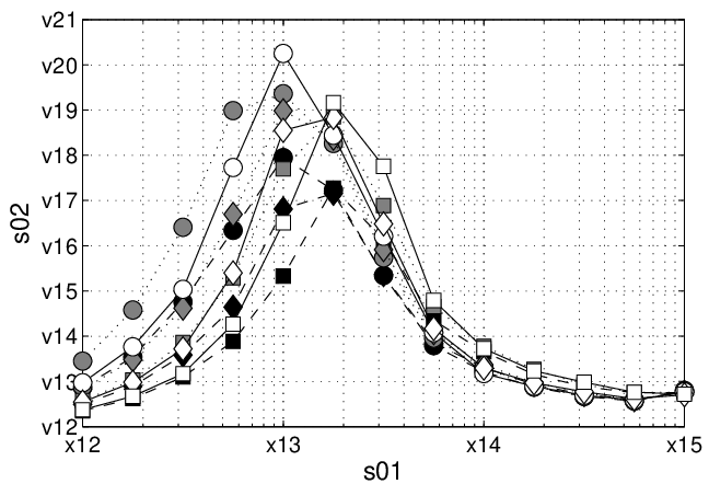
In fact, in the transition regime the STD of the alignment between and , at can be as large as 40 degrees, as shown in Fig. 4. The STD is also strongly dependent on the input SOP and on the pump power. To summarize, in the transition regime, the signal SOP is strongly pulled towards the PDG vector (see fig. 1), however the PDG vector has not yet converged to a stable, predictable configuration. Paradoxically, to improve the control and the quality of the synthesized output SOP, fibers with large randomness are to be used.
IV Conclusions
In conclusion, the polarizing properties of stimulated Brillouin scattering have been studied over a large range of PMD coefficient values in order to assess the quality and reliability of this effect for the synthesis of arbitrary states of polarization. Three regimes have been identified.
For negligible polarization mode dispersion, the polarization dependent gain vector is aligned with pump and the signal; the signal is fully polarized.
For high polarization mode dispersion, the polarization dependent gain vector tends to align to a state of polarization which has the same linear component of the pump but opposite circular component. In this regime the nonlinear polarization pulling effect, i.e. the attraction of the signal to the polarization dependent gain vector, is observed as the pump power increases. The signal is not fully polarized, though the degree of polarization tends to 1 as the pump power increases.
In the transition regime the alignment among the vectors (PDG, signal and pump) is highly stochastic; it also depends on the signal input polarization state and on the pump power; the degree of polarization is less than one.
Paradoxically, large polarization mode dispersion increases the quality and robustness of the polarization control.
References
- [1] N.A. Olsson, J.P van der Ziel, “Cancellation of fiber loss by semiconductor laser pumped Brillouin amplification at 1.55,” Appl. Phys. Lett. vol. 48, 1329, 1986.
- [2] X. Bao, D.J. Webb, D.A. Jackson, “22-km distributed temperature sensor using Brillouin gain in an optical fiber,” Opt. Lett., vol. 18, 552-554, 1993.
- [3] X.S. Yao, L. Maleki, “Optoelectronic microwave oscillator,” JOSA B 13, pp. 1725-1735, 1996.
- [4] K.Y. Song, M. Gonzalez-Herraez, L. Thévenaz, “Observation of pulse delaying and advancement in optical fiber using stimulated Brillouin scattering,” Opt. Expr., 13, 82-88, 2005.
- [5] M. Sagues, A. Loayssa, J. Capmany, “Multitap Complex-Coefficient Incoherent Microwave Photonic Filters Based on Stimulated Brillouin Scattering,” Phot. Tech. Lett., vol. 19, 1194-1196, 2007.
- [6] L. Thévenaz, ”Slow and fast light using stimulated Brillouin scattering: a highly flexible approach”, in Slow Light: Science and Applications, J. B. Khurgin, R.S. Tucker, Eds., CRC Press, 2008, pp. 173-191.
- [7] R. H. Stolen, “Polarization effects in fiber Raman and Brillouin Lasers,” IEEE J. Quant. Electron., Vol. 15, pp. 1157-1160, 1979.
- [8] M. O. van Deventer and A. J. Boot, “Polarization properties of stimulated Brillouin scattering in single-mode fibers,” J. Lightw. Technol., vol. 12, no. 4, pp. 585590, Apr. 1994.
- [9] L. Thévenaz, A. Zadok, A. Eyal, M. Tur, “All-Optical Polarization Control Through Brillouin Amplification,” Proc. OFC 2008, paper OML7, 2008.
- [10] A. Galtarossa, L. Palmieri, M. Santagiustina, L. Ursini, “Polarized Brillouin amplification in randomly birefringent and unidirectionally spun fibers,” IEEE Phot. Tech. Lett., Vol. 20, pp. 1420-1422, 2008.
- [11] A. Zadok, E. Zilka, A. Eyal, L. Thévenaz, M. Tur, “Vector analysis of stimulated Brillouin scattering amplification in standard single-mode fibers,” Opt. Expr., Vol. 16, pp. 21692-21707, 2008.
- [12] A. Galtarossa, L. Palmieri, M. Santagiustina, L. Schenato, L. Ursini, “Polarized backward Raman amplification in randomly birefringent fibers,” J. Lightw. Tech., Vol. 24, 4055-4063, 2006.
- [13] P. K. A. Wai, C. R. Menyuk, “Polarization mode dispersion, decorrelation, and diffusion in optical fibers with randomly varying birefringence,” J. Lightw. Technol., vol. 14, pp. 148-157, 1996.
- [14] B. Huttner, C. Geiser, N. Gisin, “Polarization-Induced Distortions in Optical Fiber Networks with Polarization-Mode Dispersion and Polarization-Dependent Losses,” IEEE. J. of Sel. Top. Quant. Elect., Vol. 6, pp. 317-329, 2000.
- [15] A. Galtarossa, L. Palmieri, “The Exact Statistics of Polarization-Dependent Loss in Fiber-Optic Links,” IEEE Phot. Tech. Lett., Vol. 15, pp. 57-59, 2003.
- [16] J. P. Gordon and H. Kogelnik, “PMD fundamentals: Polarization mode dispersion in optical fibers”, Proc. Natl. Acad. Sci. USA 97, 4541, 2000.