UT-09-23
IPMU09-0125
Flavor Structure in F-theory Compactifications
Hirotaka Hayashi1, Teruhiko Kawano1, Yoichi Tsuchiya1 and Taizan Watari2
1Department of Physics, University of Tokyo, Tokyo 113-0033, Japan
2Institute for the Physics and Mathematics of the Universe, University of Tokyo, Kashiwa-no-ha 5-1-5, 277-8568, Japan
F-theory is one of frameworks in string theory where supersymmetric grand unification is accommodated, and all the Yukawa couplings and Majorana masses of right-handed neutrinos are generated. Yukawa couplings of charged fermions are generated at codimension-3 singularities, and a contribution from a given singularity point is known to be approximately rank 1. Thus, the approximate rank of Yukawa matrices in low-energy effective theory of generic F-theory compactifications are minimum of either the number of generations or the number of singularity points of certain types. If there is a geometry with only one type point and one type point over the entire 7-brane for SU(5) gauge fields, F-theory compactified on such a geometry would reproduce approximately rank-1 Yukawa matrices in the real world. We found, however, that there is no such geometry. Thus, it is a problem how to generate hierarchical Yukawa eigenvalues in F-theory compactifications. A solution in the literature so far is to take an appropriate factorization limit. In this article, we propose an alternative solution to the hierarchical structure problem (which requires to tune some parameters) by studying how zero mode wavefunctions depend on complex structure moduli. In this solution, the CKM matrix is predicted to have only entries of order unity without an extra tuning of parameters, and the lepton flavor anarchy is predicted for the lepton mixing matrix. The hierarchy among the Yukawa eigenvalues of the down-type and charged lepton sector is predicted to be smaller than that of the up-type sector, and the Majorana masses of left-handed neutrinos generated through the see-saw mechanism have small hierarchy. All of these predictions agree with what we observe in the real world. We also obtained a precise description of zero mode wavefunctions near the type singularity points, where the up-type Yukawa couplings are generated.
1 Introduction
Masses and mixing angles of fermions constitute large fraction of parameters of the Standard Model that includes neutrino masses. Such flavor parameters are free coefficients of various operators in a low-energy effective field theory on 3+1 dimensions. Although one could play a game of deriving the observed flavor structure from a flavor model with a symmetry and its small breaking, quantum field theory is such a flexible framework that we can construct many models for the flavor structure of the Standard Model.
Superstring theory achieves unification of all the degrees of freedom including vector bosons and fermions, and has much stronger theoretical constraints than effective field theories. It is thus interesting what kind of insight string theory compactification could provide to understanding of flavor structure.
In unified theories with gauge group, up-type Yukawa couplings come from the interaction of the form
| (1) |
where are indices running from 1 to 5. An observation of [1] was that an underlying symmetry containing not only determines
- •
variety of representations of low-energy particles charged under
through the irreducible decomposition of - under , but also
- •
interactions among them
through the Lie algebra of ;
- •
multiplicities ( number of generations) of particles in a given representation,
however, are not determined from the underlying symmetry and its breaking pattern to . The multiplicities, often regarded as one of the most important clues in search for microscopic descriptions of elementary particles, are determined by topology in geometric compactifications of string theories, not purely from algebra (symmetry breaking). Thus, by ignoring the information of multiplicities and by focusing both on the type of representations and their interactions, one can determine the underlying symmetry and its breaking pattern to . This is a natural generalization of the determination of chiral symmetry behind the physics of pions. In the case of unified theories, at least is necessary as an underlying symmetry. If one tries to generate all other particles in supersymmetric Standard Models and all the Yukawa couplings from a single underlying symmetry,11 1 In generic F-theory compactifications, though, this assumption does not have to be imposed. See [2, 3], or discussion around eq. (24) in this article. is the minimal choice [1]. See also [4, 5] for recent articles.
Although underlying symmetries can be inferred from low-energy data, other inputs, either experimental or theoretical, are necessary to find out how the underlying symmetries are implemented (like QCD!); without a firm theoretical implementation, underlying symmetry alone can not do very much. In super string theory, we can spot three frameworks where and other exceptional type symmetries can be implemented. They are Heterotic string theory, M-theory compactified on holonomy manifolds and F-theory. Moduli space of these frameworks partially overlap with one another, but not entirely. Even in overlapping region of moduli space, analysis of low-energy physics may be easier in one framework than in the other. In F-theory compactifications (to be more precise, in region of moduli space where there is no Heterotic or M-theory dual, or where F-theory provides an easier way of analysis) charged matter fields are known to have wavefunctions localized in internal space, and flavor structure can be studied in a relatively intuitive way. This is why we study flavor structure in F-theory compactifications.
Study of flavor structure begins with understanding how to read out the low-energy degrees of freedom and their properties (wavefunctions in the internal space) from geometric data for F-theory compactifications. There has been a considerable progress in this direction in the last two years [6, 7, 8, 2, 9, 3]. An F-theory compactification with supersymmetry in 3+1 dimensions is described by a Calabi–Yau 4-fold that is an elliptic fibration over a complex 3-fold . It has been known since 90’s that gauge fields are localized on complex surfaces in , and charged matter fields are localized on complex curves in the surfaces, but now we further know that all the massless modes of charged matter fields22 2 By “all” the charged matter fields, we only mean those in , , and representation of , , and representations of , and and representations of . Those fields (and of ) are the minimal matter contents. When , matter fields in appear when the irreducible piece of discriminant locus develops an extra singularity (see e.g. [10]). correspond to smooth wavefunctions on the complex curves; although there are multiple points of enhanced singularity types along the complex curves, none of the charged matter fields are specifically associated with the singularity points [8].33 3 This is a pedagogical expression of a statement that all the charged matter fields are global holomorphic sections of some line bundles, not of a sheaf with torsion components associated with singularity points. It was far from obvious whether this statement was true; see e.g. [11] or [6].,44 4 This result has an immediate application to phenomenology. The absence of torsion components was a crucial input in making predictions on the branching fraction of dimension-6 proton decay ([12] and version 3 of [13]). It is also known how to determine the smooth wavefunctions on the complex curves [8]; we will review the technique with some explicit examples in section 3, and elaborate more on the technique in this article.
Charged matter fields are regarded as M2-branes wrapped on vanishingly small 2-cycles along the complex curves (called matter curves), and Yukawa couplings are re-wrapping process of M2-branes that preserve the sum of topological 2-cycles. Examining the algebra of topological 2-cycles, it turns out that the up-type Yukawa couplings and down-type Yukawa couplings are generated [1], presumably55 5 Discussion in section 4.5 will make it clear why we keep the word “presumably” here. at around singularity points in where the singularity is enhanced to and , respectively [7, 6, 8]. Since F-theory does not have microscopic quantum formulation, it is hard to imagine how Yukawa couplings associated with singularity points can be analyzed quantitatively without microscopic theory describing geometry around the singularity points. References [14, 6, 7], however, developed an effective description of gauge-theory sector using field theory on 7+1 dimensions, and proposed to use it to study Yukawa couplings. Although microscopic formulation of F-theory is not known yet, the idea is that such unknown effects can be incorporated as higher-dimensional operators in the field theory Lagrangian, with unknown coefficients; as long as we are interested in far infra-red physics such as Yukawa couplings below the Kaluza–Klein scale, leading order terms will be the most important. Despite unknown coefficients of the higher-order operators, such effects must be power suppressed, and influence on the low-energy observables (such as masses and mixing angles) should be estimated (by order of magnitude). In this program, geometry of needs to be translated properly into the background field configuration of the effective field theory on 7+1 dimensions. Physics and mathematics involved in this translation was (almost) clarified in [2, 9] and references therein66 6 The process of translation is not trivial. For example, the linear configuration of with quotient, adopted e.g. in [15] turns out not to be correct (see appendix of [3] for more information). We will add a little more material to this translation process in the appendix C in this article.
Now we know how to calculate smooth wavefunctions of massless modes, how to calculate Yukawa couplings from individual regions around singularity points by using field theory models for the local geometry, and how to combine these two techniques [2]. It turns out that contribution to the up-type Yukawa matrix from a region around an -type singularity point is approximately rank-1 [2], and that to the down-type Yukawa matrix from a region around a -type singularity point is also approximately rank-1 (e.g., [7]).
Such studies, however, do not make a clear distinction between (down-type Higgs multiplet) and (left-handed lepton doublets). Any sensible theories of flavor structure in supersymmetric compactifications should have a framework where dimension-4 proton decay operators are brought safely under control. Since the vanishing dimension-4 proton decay operators is about vacuum value of moduli, and since right-handed neutrinos are identified with fluctuations of moduli fields from vacuum, the dimension-4 proton decay problem and how to generate Majorana masses to right-handed neutrinos are deeply related issues. Three frameworks were proposed in [3] (two of which were essentially carried over and generalized from [1]):
- •
matter parity: perhaps the most natural scenario to many people. Geometry of and 4-form flux background should be arranged so that a symmetry remains unbroken. Various matter fields at low-energy should come out with the right assignment of the parity ( transformation law). Majorana masses of right-handed neutrinos are generated automatically in flux compactifications. Flux compactification of F-theory predicts the scale of the Majorana mass somewhat below the GUT scale, which is phenomenologically favorable. (section 4.1 of [3])
- •
factorized spectral surface with an unbroken U(1) symmetry: Complex structure of needs to be tuned so that the spectral surface factorizes [1]. Ultimately the factorization has to be specified in a global geometry, because the factorization only at quadratic order may not be sufficient to get rid of the proton decay operators (c.f. section 4.3.3 of [3]). Reference [16] (implicitly) proposed to tune complex structure parameters further so that an Higgs bundle is defined globally on a complex surface for the unified theories, so that the global factorization of spectral surface can be discussed within the canonical bundle . In the presence of an unbroken U(1) symmetry in the factorization limit, the dimension-4 proton decay operators are forbidden, but at the same time, the Majorana mass of right-handed neutrinos are also prohibited at perturbative level [16], when the symmetry is broken either by a Wilson line [17] or by a flux in the hypercharge [17, 13, 18].77 7 Whether a vector boson associated with this U(1) symmetry remains massless or not depends on global aspects of compactification geometry (including fluxes). If it remains massless down to low-energy, there are other phenomenological problems. i) the U(1) vector boson has to be Higgsed at some scale above the experimental bound, ii) one needs an idea what sets the scale of the “Higgs mechanism” of the U(1) vector field, iii) 1-loop mixing between the extra U(1) and of the Standard Model change the running of gauge coupling constants and ruin the prediction of gauge coupling unification, if the extra U(1) vector field remains massless down to low-energy, and finally, iv) it is Higgsed at high-energy, then the U(1) symmetry is not effectively solving the dimension-4 proton decay problem.
- •
spontaneous -parity violation: factorized spectral surface with non-zero Fayet–Iliopoulos parameter. A safe way to break this unwanted U(1) symmetry while keeping the proton decay operators from being generated is to trigger spontaneous breaking of the U(1) symmetry (and Higgsing of the vector field) by non-zero Fayet–Iliopoulos parameter [1, 19]. Majorana mass of right-handed neutrinos are also generated. (section 4.4 of [3])
Now all the necessary theoretical tools and frameworks are available; time is ripe, and we are ready to study flavor structure in F-theory compactifications.88 8 This article does not study the flavor structure in the third framework, however, because we do not have enough theoretical tools yet. Our goal is to clarify which parameters can be tuned99 9 We tune them by hand, for now; hoping someday that the tuning is justified by flux compactification or phenomenological/cosmological considerations. to reproduce known flavor structure, and which aspects of flavor structure are derived theoretically.
This article is organized as follows. Yukawa matrices of low-energy effective theory are given by summing up contributions from all the codimension-3 singularity points. An idea of [15] is to assume that there is only one codimension-3 singularity point of a given type to reproduce hierarchical structure among Yukawa eigenvalues. But this assumption is not satisfied generically, and furthermore, we found in section 2 that this cannot be satisfied.
Thus, we have to take account of all the contributions from different codimension-3 singularities, and we need to be able to evaluate which contribution is more important relatively to others. For this purpose, we take a moment in section 3 to present a technique of how to calculate wavefunctions of zero modes along the matter curves.
The zero mode “wavefunctions” are not “functions”, but are sections of some bundles. Thus, an extra care has to be taken in describing the “wavefunctions”. In section 4, a clear distinction is introduced among descriptions of the sections in holomorphic frame, unitary frame and diagonalization frame. In order to determine physical Yukawa couplings in the low-energy effective theory, both the kinetic terms and tri-linear (Yukawa) couplings need to be expressed in terms of wavefunctions in a certain frame; clear distinction among different frames is crucial in writing down the expression for the kinetic terms. This conceptual clarification achieved in section 4 enables us to take on a problem of providing a better field-theory description of “branch locus” that appears in local geometry with enhanced , and singularity. Progress beyond [8, 2] is presented in the appendix C.
We will study in section 5 how the “wavefunctions” in unitary frame change when some complex structure parameters are changed. It is only a case study of simple examples, is not meant to be a thorough or extensive one. But, at least, the study shows that zero mode wavefunctions get localized within the matter curves for certain choices of complex structure parameters.
Yukawa matrices of low-energy effective theory of F-theory compactifications are generically predicted not to have hierarchical structure. That is a problem. We show in section 6 that this problem can be solved by the localized wavefunctions found in section 5. Small mixing structure of the CKM matrix partially follows as a consequence of this localized wavefunctions, without an extra tuning of moduli parameters.
Section 7 is devoted to summary and discussion. Two solutions to the hierarchical structure problem of Yukawa eigenvalues are given in this article: one is not written elsewhere in this article and the other is the one in section 6. Their summary and comparison are given in this section. We also briefly comment on another solution to the hierarchical structure problem that is already mentioned in [20, 16].
The appendix A is a side remark. The moduli map between the Heterotic string theory and F-theory is often written down in a form that includes only the visible (or hidden) sector bundle moduli, but not the other. We wrote down a map that includes both, and show that the “stringy corrections” to the locus of -type codimension-3 singularity points vanish for Heterotic–F dual models at any points in the moduli space.
Reading Guide Sections 6, 7 and this Introduction are written in as plain language as possible. We believe that they are accessible to non-experts including phenomenologists. Section 6.1, on the other hand, is intended to be a review of basic things in flavor structure for string theorists.
Section 4 provides conceptual clarification, while sections 3 and 5 solve technical problems, and overall prepare for section 6. Section 6 itself, however, can be understood in an intuitive way, and it is an option to skip these technical sections 3–5.
Basic concepts and ideas covered in section 3 have already appeared in [8, 17, 9, 3, 16, 21]. Section 3 elaborates a little more on them by using explicit examples, and tries to make them more accessible. Geometry associated with matter parity is discussed in section 3.2.4 in much more detail than in [3]. Thus, we hope that some of the contents in section 3 will be useful from the perspective of “geometric engineering” of the Standard Model, although the engineering of the Standard Model is not the primary subject of this article.
2 Topological Invariants of Matter Curves
In an F-theory compactification with the grand unification group , the up-type Yukawa matrix gets contributions from all the -type singularity points with approximately rank-1 [2] from each of the singularities. On the other hand, all the -type singularity points contribute to the down-type Yukawa matrix with approximately rank-1 [17] from each of them. It suggests that in the F-theory compactification with the number of generations , the up-type and down-type Yukawa matrices are of approximately rank and , respectively, where and are the number of -type and -type singularity points, respectively, in the GUT divisor .
The number of points of each type singularity is a topological invariant, and cannot be tuned by hand. The number of -type points is not generically one [8], but the up-type Yukawa matrix in the real world is known to be approximately rank-one, in that the top-quark Yukawa eigenvalue is of order one, and all others are much smaller. A proposal of [15] is that there must be an F-theory compactification where and are both one in . In this section, however, we will raise a question whether such a geometry with such a topology ever exists.
We begin, however, with a brief review on matter curves in an F-theory compactification with the grand unification groups and , while setting up notations. Those familiar with the contents in [22, 10, 23, 1, 8, 9] can proceed to p.2.
An F-theory compactification to 3+1 dimensions is described by specifying a Calabi–Yau 4-fold that is an elliptic fibration on a complex 3-fold :
| (2) |
Let the elliptic fibration be given by a Weierstrass model
| (3) |
where and are holomorphic sections of and , respectively, when an unbroken supersymmetry is required below the Kaluza–Klein scale. To obtain an and unification in the F-theory compactification, the set of the zero loci of the discriminant
| (4) |
needs to contain an irreducible component with multiplicity 5 and 7, respectively, and the singularity of in the transverse direction of is and , respectively, on a generic point of . We call this in as the GUT divisor.
Charged matter chiral multiplets are localized on matter curves. For unified theory models, a 6D hypermultiplet in the representation is localized on a curve in and a 6D hypermultiplet in the representation on a curve in . For unified theory models, a 6D hypermultiplet in the spin and its conjugate representation is localized on a curve , and one in the vector representation on a curve in . It might appear at first sight that these curves may be in any topological classes of , by arranging their “7-brane” configurations in . In fact, there are not much freedom. One can show in a generic F-theory compactification that once a normal bundle on is assumed, then no other freedom is left; this follows by requiring both box anomaly cancellation in any compact 2-cycles and the topological condition of “all the 7-branes” (4) [10, 23, 1, 9].1010 10 In Calabi–Yau orientifold compactifications of Type IIB string theory with only D-branes and orientifold planes, the box anomaly cancellation and the topological condition (4) both correspond to a single condition; the Ramond–Ramond charge cancellation (Bianchi identity) associated with the Ramond–Ramond 0-form field. In F-theory in general, however, these two conditions are not the same. Conventionally a divisor on is defined [24]1111 11 To our knowledge, this was the first reference to try to define only from geometric data around , so that the definition does not depend on the global topological aspects of . from the normal bundle by
| (5) |
Using this divisor , topological classes of the matter curves are given by
| (6) | |||||
| (7) |
An easier way to see this is to take a local patch of , so that there is a normal coordinate of in . In order to obtain a split singularity along , the defining equation of should locally look like [22]
| (8) | |||||
In order to obtain a singularity, should also vanish. Because and are sections of and , respectively, to be glued together over , they behave near as sections of
| (9) |
respectively. Thus, all the terms in (8) should also be sections of . Since the normal coordinate is a section of , one can see that
| (10) |
for . Once the normal bundle (and hence the divisor ) is specified, all the line bundles for ’s, ’s, and so on, are determined.
The discriminant becomes1212 12 technical note: Let us explain how is related to in [8], in version 4 of [8] and in [3]. First, (11) vanish in an F-theory compactification that has a Heterotic dual, and hence and become and , respectively. See also the appendix A for more details. and are modified from and , respectively, by (12) Since it is the location of zero points of or on the curve that is directly relevant to low-energy physics, the modification by above does not make a practical difference. As the “branch locus” of the spectral surface , however, and are the correct expression. When a limit (24) is taken, a result in [9] is obtained from .
| (13) |
| (14) | |||||
| (15) | |||||
The matter curves and correspond to and , respectively, and they are in the topological classes specified in (6), because and are sections of the line bundles specified by the divisors in (6). In unified theory models, the discriminant indicates two matter curves, and , on the divisor . Similarly, one can see that the two curves are in the topological classes in (7), because and are sections of the line bundles and , respectively.
An important point is that all the topological classes of matter curves have already been determined, when the complex surface of generic singularity type and the first Chern class of the normal bundle are specified. Alternatively, one can specify a topological class of for (or for ), instead of the first Chern class of . In Table 1, we showed several examples of topological choice of the GUT divisor of singularity and the matter curve . All the topological invariants in the 3rd–7th column are determined, once the topological classes in the first and second columns are specified.
| # | # | # | Ref. | |||||
|---|---|---|---|---|---|---|---|---|
| I | 0 | 2 | 4 | 104 | 298 | [8] | ||
| II | 0 | 0 | 1 | 89 | 262 | [8] | ||
| III | 0 | 4 | 7 | 119 | 334 | [8] | ||
| IV | 0 | 6 | 10 | 134 | 370 | [9] | ||
| V | 0 | 6 | 10 | 124 | 340 | [20] | ||
| VI | 0 | 4 | 7 | 129 | 364 | |||
| VII | 0 | 10 | 16 | 174 | 472 | |||
| VIII | 1 | 18 | 27 | 226 | 594 | |||
| IX | 3 | 28 | 40 | 285 | 730 | |||
| X |
The 4th and 5th columns give the numbers of codimension-3 singularity points on where the singularity is enhanced to and , respectively. An -type singularity point is given by a common zero of the pair (, ), while a -type singularity point is given by a common zero of the pair (, ), and their numbers are thus given by
| (16) |
The genus of the matter curve for the representation and that of the covering matter curve for the representation are given by
| (17) | |||||
| (18) | |||||
| (19) |
Since an -type singularity point is a common zero of and and is not a -type singularity [8] (and its v4),
| (20) | |||||
| (21) |

All these numbers are topological, and cannot be changed by tuning moduli parameters. In all the examples in Table 1, the number of -type and -type singularities are not 1 in any one of the examples.
In fact, from the expression of and , one can see that
| (22) |
The number of -type singularities is always even; it cannot be 1. The number of codimension-3 singularity points is a crucial element of flavor structure of Yukawa matrices of low-energy effective theory. An idea of Ref. [15] was to assume a geometry with for a compactification, in order to realize an approximately rank-1 up-type Yukawa matrix of the real world. Now we know, however, that this idea does not work.
One might think of taking a limit of the complex structure by hand, so that the matter curve factorizes into irreducible pieces in the GUT divisor .
| (23) |
Only one of the irreducible pieces, say, , may be regarded as the support of fermions of the Standard Model. Similarly, the matter curve may also factorizes into irreducible pieces, , and only one of them, say, is regarded as the support of fermions of the Standard Model. If the factorization limit is chosen properly, then there may be just one -type and one -type intersection points that involve the relevant pieces or/and [20]. The idea of [15] may still be valid in this context [20].1313 13 Some articles (e.g., [25]) derive predictions on flavor structure in the lepton sector under an assumption that there is only one point in the GUT divisor where the matter curve and the Higgs curve intersect. The number of this type of intersection points, however, is also a topological invariant, and is expressed in terms of intersection numbers of divisors on . In the appendix B, we determined the numbers of all sorts of codimension-3 singularities in terms of intersection numbers in the case a 5-fold spectral cover (that we state shortly in the main text) factorizes into a 4-fold cover and a 1-fold cover.
Such a factorization limit of the curves may exist, but a factorization of a matter curve does not always imply that independent massless fields can be classified into irreducible pieces of the reducible matter curve based on their support [3]. In order to make sure that the Standard Model fields e.g. in the representation localizes on only one irreducible piece of the factorized matter curve , not only the curve, but also its spectral surface needs to be factorized. Furthermore, in order to achieve a well-defined factorization (see section 4.3.3 of [3]), one needs to take the limit in
| (24) |
to make sure that an Higgs bundle is well-defined globally on , as implicitly done in [16]. The higher order terms in the -series expansion in (8) surely become irrelevant in this limit,1414 14 Introduce a new set of coordinates () satisfying , and . This is to look into a region near closely. In the new coordinates, the equation (8) becomes (25) which is an equation of a deformed singularity with negligible terms of order . The two-cycles with the intersection form stay within the range of , and , where higher order terms are negligible. and we are sure that there is a set of 2-cycles with the intersection form of fibered globally over . In the presence of an unbroken U(1) symmetry in such a factorization limit, the Majorana mass of right-handed neutrinos is forbidden by this U(1) symmetry, if the up-type Higgs and down-type Higgs multiplets are vector-like in , which is the case if the symmetry is broken either by a hypercharge Wilson line associated with [17], or by a hypercharge line bundle [17, 13, 18], as pointed out in [16]. One also has to make sure that all kinds of physics associated with -charged non-Standard Model matter fields on and do not conflict against low-energy phenomenology.
If we want to maintain the successful prediction of Majorana masses of right-handed neutrinos in the matter parity scenario [3], on the other hand, we cannot rely on a globally defined Higgs bundle or vacuum with an unbroken U(1) symmetry. In this case, the up-type Yukawa matrix of the effective theory may have contributions from more than one -type singularity points. Clearly, the idea of [15] does not work in this case. In order to evaluate the flavor structure of Yukawa matrices that involve contributions from multiple points in the GUT divisor , we need to know how the zero mode wavefunctions behave along the matter curve. This is what we study in the next three sections.
Before moving on to the next section, let us pause for a moment to pose the following question, which we think is interesting at least in the context of model building. In all the examples in Table 1, the matter curve for the representation – has a very large genus.1515 15 It should be fair to mention that this large genus of the matter curve for the representation was already known in [26]; the genus of a matter curve is determined only by the choice of , in F-theory as well as in elliptically fibered compactifications of Heterotic strings, and hence the result in [26] should be regarded as the same phenomenon as in Table 1. The question is if that is a generic feature of F-theory compactifications. If it is generic, we should think of phenomenological consequences of this feature.
To address this question, note that the right-hand side of (19) can be reorganized as
| (26) |
Since the first term is proportional to , it is always zero or positive. The second term is positive when the anti-canonical divisor is ample,1616 16 This is the case when with . is marginal, in that the second term can also be zero. because containing is effective. Finally, in the last term, is 8 for all the Hirzebruch surfaces , and is for the del Pezzo surface . Thus, unless for del Pezzo surfaces, the last term is always positive with the large coefficient 20. All the three terms are positive, with their relatively large coefficients 7, 9 and 20. It is now easy to see why the (covering) matter curve of the representation – tend to have very large genus in the examples of Table 1; the last term alone contributes by for , and for .
We can also learn another lesson. The term becomes small, for example, for with larger . See Table 2.
| # | # | # | |||||
|---|---|---|---|---|---|---|---|
| XI | 0 | 0 | 1 | 19 | 52 | ||
| XII | 0 | 0 | 1 | 9 | 22 | ||
| XIII | 0 | 0 | 1 | 19 | 52 | ||
| XIV | 0 | 2 | 4 | 24 | 58 | ||
| XV | 0 | 2 | 4 | 24 | 58 | ||
| XVI | 1 | 4 | 6 | 31 | 72 | ||
| XVII | “1” | 2 | 3 | 16 | 36 |
By using or , the genus of can be reduced from to at least . The large genus of the matter curve in the representation of , therefore, is not a generic prediction of F-theory compactifications, but it is an artifact of in the Hirzebruch series and the del Pezzo series with small .
On a complex curve with a large genus , a line bundle with a negative degree does not have non-zero . Those with do not have non-zero , either. For bundles in the range , however, both and can be non-zero. Such massless fields in a pair of vector like representations may be identified with the two Higgs doublets of the supersymmetric Standard Models [17] or messenger fields in gauge mediation of supersymmetry breaking. For larger , the window for becomes larger. Too many extra pairs of chiral multiplets in the representation 5 (See [26]) will change the running of the gauge coupling constants too much and are not acceptable to retain a perturbative gauge coupling unification. Thus, a large genus does not seem to be a favorable situation. The observation so far, therefore, might be taken as an indication that with a large is a favorable choice phenomenologically.
The authors are clearly aware, however, that things are more complicated than that, and we have just scratched the surface of possible choices of topology. A choice of topological class of and that of set a constraint on the smallest possible net chirality, and on the choices of fluxes to achieve it. The genus is already determined from the topological data of and . The number of unnecessary pairs is determined not by the genus alone but also by the choice of fluxes that has already been constrained tightly to reproduce the net chirality . This problem is a bit complicated, and we will not point to a particular direction to search for a geometry giving rise to the Standard Model. In this article, therefore, we just note that the genus of the curve depends strongly on , and that the genus becomes smaller for smaller .
| (a) | (b) | (c) |
|---|---|---|
 |
 |
 |
3 Holomorphic Wavefunctions on Matter Curves
We have seen that the number of -type codimension-3 singularity points is more than one, and the up-type Yuakwa matrix of low-energy effective theory receives contributions from more than one local patches on . It is therefore necessary to calculate the zero-mode wavefunctions over the compact matter curve , so that one can argue relative importance of contributions to Yukawa couplings from multiple codimension-3 singularity points on .
A zero mode chiral multiplet is identified with a holomorphic section of a certain line bundle on a matter curve, and a divisor specifying the line bundle is determined from the loci of codimension-3 singularity points [27, 11, 8]. It must be therefore straightforward to calculate the number of independent zero modes, and to determine their wavefunctions as holomorphic sections on the covering matter curve. We think, however, that it is worthwhile to illustrate it with concrete examples, and that is what we will do in this section.
3.1 Global Holomorphic Sections
A zero mode chiral multiplet of a charged matter field correspond to a global holomorphic section of a line bundle on a matter curve. Here, we give a short brief review of relevant mathematical materials, partially as a guide to readers unfamiliar with them, and partially for the purpose of setting up notations.
In order to describe global holomorphic sections of a line bundle on a manifold/variety , one chooses an open covering of ; . A rational function on each is chosen to describe the divisor , so that
| (27) |
It follows that neither nor should have a pole or zero in , so that (27) in is consistent with the one in . is called the Cartier divisor description of the divisor . The open covering plays the role of trivialization patches of the line bundle ; although the cohomology group
| (28) |
is primarily described by a set of rational functions on , one can assign a holomorphic function on for an element of . The holomorphic functions and in the overlapping patch are related by ; thus, plays the role of the transition function from to of the line bundle . The holomorphic function on is the coefficient function in the component description in the individual trivialization patches (there is only one component because we are talking about a rank-1/line bundle). Thus, the zero mode wavefunction can be described by specifying an open covering , transition functions on , and a holomorphic function on each glued together consistently by the transition functions.
The description in terms of and does not change when the divisor is replaced by with a rational function on , one that is linearly equivalent to the original divisor . One can use in a Cartier divisor description of , but . Further, since , .
The wavefunctions , however, do depend on the choice of divisor class (divisor modulo linear equivalence), not just on the first Chern class of the line bundle . (Here, we now consider a case where of is a curve.)
Let us see this in one of the simplest examples. We take an elliptic curve given by1717 17 The coordinates and have nothing to do with and in (8).
| (29) |
and consider a line bundle specified by a point . The divisors and (both ) are not linear equivalent if . Let us see explicitly that a global holomorphic section of depends on the choice of the divisor class .
For a given , the elliptic curve can be covered by three patches
| (30) |
where is the zero element in the Abelian group structure on . is the summation of the group law on , and for denotes the inverse element of of the group law. An arbitrary point can be used in defining above. in the definition of is a point satisfying .
Let us construct a rational function on each to give a Cartier divisor description of the divisor . On the patches , where the point is removed, we can choose as constants, i.e., , . On the other hand, should have a zero of order one at and have no other zeros or poles anywhere on the patch . In order to have a zero at , we can choose . has a zero at and at , and a second order pole at . But a second order pole is irrelevant since the patch does not include the origin . On the other hand, we have to cancel the zero at . To this end, we divide by where . has a zero of order one at , a zero of order two at , and a pole or order three at . The zero of order two at can be understood from the fact that the group-law sum of the zero points of an elliptic function is the same as that of the poles. The zero of order two at and the pole of order three at are also irrelevant on the patch , and the zero at of the denominator cancels the zero at of the numerator . Thus, a rational function has a zero of order one at , and no other zeros or poles in . This function can be used for .
As a whole, the rational functions () for the Cartier divisor description of can be chosen as
| (31) |
with .
Since in the sense of (28) consists of only one rational function (mod ), , the generator of the vector space of zero mode(s) correspond to a holomorphic wavefunction . Clearly the wavefunction depends on the choice of .
3.2 Example VII
Let us choose the example VII in Table 1, first. This is one of the easiest examples, and will be suitable for illustrative purpose.
In the example VII, the GUT divisor is , and the matter curve is in the topological class , where is a hyperplane of . The explicit choice of —a homogeneous function of degree two of the homogeneous coordinates—determines the curve in . When are also chosen from their appropriate line bundles, the curve is also determined by as a subvariety of . Figure 2 illustrates the configurations of the matter curves in Example IV for different complex structures.
3.2.1 Fluxes for Chirality: Set-up for Calculation
We cannot talk about the chiral matter contents in the low-energy effective theory below the Kaluza–Klein scale without introducing 4-form fluxes in the Calabi–Yau 4-fold . The net chirality of a pair of Hermitian conjugate representations of unbroken symmetry is determined by integrating the 4-form flux over the vanishing 2-cycle parametrized by the covering matter curve [8].
An available 4-form flux depends on the choice of Calabi–Yau 4-fold. It cannot be determined only from the geometry of the GUT divisor and its infinitesimal neighborhood in the base 3-fold . For a given 4-fold , one needs to identify the available flux in , and further finds out how individual generators of this cohomology group contribute to the 4-cycle of vanishing 2-cycles over (covering) matter curves of various representations in . That is what one is supposed to do to search for the geometry describing the real world, and that is an area where more technical development is yet to be necessary.
We know, however, that the 4-form flux background on is once encoded as line bundles on spectral surfaces of various representations. Line bundles on matter curves are obtained from restriction of the line bundles on the spectral surfaces. The wavefunctions of zero modes are determined by using the line bundles on the matter curves. Thus, as an intermediate step, it is possible to assume a certain form of a line bundle on a spectral surface, and study the consequences; such approach does not guarantee that a set of a 4-fold and a 4-form exists for the assumed line bundles on the spectral surfaces. In this intermediate step approach, the existence proof—also known as “swampland program”—can be put aside as an open problem, and the remaining half of the problem can be addressed separately. We do not necessarily mean that this is the best strategy, but at least for the purpose of illustrating how to calculate the wavefunctions of the zero modes, we consider that it is wise to start from the intermediate step, instead of doing everything in a top-down approach from the first principle. We will thus consider consequences of a hypothetical 4-form flux on a hypothetical variety by assuming a line bundle on each of all the spectral surfaces.
The GUT divisor is covered by open patches , where field theory local models are defined. When a local geometry of in a neighborhood of is approximately described by an ALE fibration of type where is one of the series, then the physics associated with this ALE fibration is described by a field theory local model on with the gauge group . The choice of the gauge group may, in principle, be different for different patches in [2, 3]. Here, however, for illustrative purposes, we choose a specific choice (limit) of the complex structure, so that the GUT divisor is covered by a single field theory local model, whose gauge group is . That is the case, for example, when the limit (24) is chosen in an F-theory compactification (this includes an F-theory compactification with a Heterotic dual, and the complex structure moduli are in the stable degeneration limit.) In that case, a spectral cover for the representation of the unbroken symmetry is a divisor of , and a 5-fold cover over . We assume a line bundle on in a form
| (32) |
where is the ramification divisor associated with the projection , and the divisor on is given by
| (33) |
is regarded as a divisor within in the first term of (33), while in the second term, it is regarded as a divisor on , and is pulled back to by the projection . In terms of a fiber coordinate of , the former is given by , and the latter by . This divisor is chosen so that in . This line bundle on the spectral surface was developed originally in a description of Heterotic string compactifications [28], but now we know that the spectral surface and a line bundle on it are readily used for F-theory compactifications as well [2, 9].
We are fully aware that this is by no means a generic choice of the complex structure of or of flux on it. Higgs bundles via the extension construction, or Higgs sheaves in that are not represented as a pushforward of a line bundle on the spectral surface in [3]1818 18 An F-theory compactification using such a background may be used for a framework of phenomenologically viable R-parity violation. cannot be covered in this way of incorporating a flux background. But for now, we will content ourselves with working out zero-mode wavefunctions for a limited class of choices of background.
3.2.2 Zero Mode Wavefunctions in the Representation –
Now all the relevant data are set, and we are ready to calculate zero mode wavefunctions. We will first identify independent zero modes in (and possibly in ) of , and then determine their wavefunctions. The vector space of zero modes in the representation is given [27, 11, 8] by
| (34) |
The divisor on is restricted on , and so is the divisor on . stands for the collection of all the codimension-3 singularity points of the -type singularity enhancement (also called type (a) points in [8]). All the information of the divisor class of the line bundle is retained in (34), not just the degree of this line bundle; this expression can be used in calculating the wavefunctions.
In order to study this line-bundle valued cohomology group, we need to know the divisor on the curve very well. There is no problem with the restriction of or , but we have a bit more work with the restriction of .
The divisor in has two irreducible components. One is itself, and the other is a collection of points of that is projected to , but are not on the zero section of . The first component has a coefficient , and the second one . In order to provide a more intuitive understanding of this divisor, let us focus on a region of around a point of -type codimension-3 singularity. Let the local defining equation of the spectral surface be
| (35) |
where , and is a fiber coordinate of . can be chosen as a set of local coordinates of , while it is more appropriate to take as the local coordinates on ([8, 2]). The divisor in is described in this local region in this set of local coordinates as
| (36) | |||||
The first component corresponds to , and the second one to . See Figure 3.
 |
 | |
| (a) | (b) |
The first component div() is right on the matter curve , while the second one intersects transversally with the matter curve at the -type singularity point , and hence at on .
When a divisor of is restricted on , the divisor becomes a collection of intersection points of and (with the multiplicity of an intersection as the coefficient of the intersection point). The collection of these points defines a divisor on the matter curve . This definition of restriction is readily applied to the second component div() of , but not to the first one div(), because the intersection point or the multiplicity of the intersection is not well-defined, when is restricted onto itself. Thus, we replace by another divisor of that is linearly equivalent to , and move the first component of away from the matter curve . Let us take an arbitrary holomorphic section of that is different from . Then is a rational function on . We define a divisor by1919 19 is not a rational function but a holomorphic section, and it is not conventional to use such a notation as . Its meaning will be clear, however. That is the zero locus of the section . We will use this notation in this article.
| (37) |
and use this one instead of . Now
| (38) |
Now all the components of the divisors on the matter curve are understood.
The -type singularity points on are characterized as the zero loci of on . Therefore, they give the divisor on the matter curve for the line bundle
| (39) | |||||
which can be regarded as a divisor on restricted onto the matter curve .
Since the sheaf cohomology group of our interest is of the form
| (40) |
and since is a divisor of a complex surface , we can use the short exact sequence
| (41) |
in calculating the cohomology group of our interest. The long exact sequence of their cohomology groups is
| (42) |
Thus, the cohomology groups on the matter curve can be obtained from the line-bundle valued cohomology groups on .
Let us now take a specific value of . We will use in order to minimize the net chirality, though it does not give the realistic number of the generations ([27])
| (43) |
Models with are certainly not “realistic”, but we will keep carrying out this calculation, because this is only for illustration of the basic techniques, and the generalization or application to other cases will be straightforward.
When ,
| (44) | |||||
| (45) |
Since (for ), and , we find that
| (46) |
that is, there is no massless chiral multiplets in the representation of , and
| (47) |
Since the map on the right hand side of (47) is an injective map from the -dimensional space to the -dimensional space, the cokernel is a -dimensional space, which is the same as we expected from (43).
Our goal here in this section, however, is not just to obtain the number of independent massless fields in representations and separately. As long as we use the form of flux (33) on a spectral surface of an Higgs bundle globally defined on , what we have done so far is not different from the corresponding analysis in Heterotic string compactifications on elliptically fibered Calabi–Yau 3-folds, and the necessary techniques have been well established. We proceed further, in this article, and determine (holomorphic) wavefunctions of the independent massless fields on their matter curves. In F-theory compactifications, a zero-mode wavefunction can be described on a complex curve (or on the complex surface ); we do not have to deal with a wavefunction on the complex 3-fold base like on a Calabi–Yau 3-fold in a Heterotic compactification, and this makes our task easier.
Let us describe and in the way we explained with in section 3.1. For , we choose an open covering of as , where , and and are defined similarly. A Cartier divisor description of is given by
| (48) |
whereas for a Cartier divisor description of , a rational function for it on each patch is given by the rational function for shifted by on the same patch, because is the zero locus of , and thus
| (49) |
Note that is regarded as a homogeneous function of degree five of the homogeneous coordinates of , and as homogeneous functions of degree two. The transition functions for the line bundle are given by on , on , and on . For , they are given by on , on , and on .
A global holomorphic section of a line bundle corresponds to a rational function on for the divisor ; for and , their rational functions are of the forms
| (50) |
respectively, where and are homogeneous functions on of degree 6 and 8, respectively. is regarded naturally as a subset of , because is effective; to be more explicit, can be regarded as a special form of . Since the zero mode matter fields are given by (47), the zero mode wavefunctions are identified with ; this is quite reasonable, because this says that only on – on the locus – is relevant. In the description using the trivialization patches, zero modes in the representation have wavefunctions on given by
| (51) |
Classes of holomorphic functions on , and above correspond to uniquely defined holomorphic functions on , and . These wavefunctions do not depend on the choice of , but on its divisor class. One can arbitrarily choose independent ones among to specify a basis in the dimensional vector space of the zero modes in the representation .
3.2.3 Zero Mode Wavefunctions in the Representation –
Let us now move on to calculate the wavefunctions of zero modes in the representation –. The vector space of chiral multiplets in the representation is [26, 29, 8]
| (52) |
Here, resolves all the double points of at the -type codimension-3 singularities, and pulls back from to the covering matter curve . denotes the divisor consisting of all the -type singularity points on , which is given by the zero locus of except the -type singularity points (which are on the locus ) [8]. Strictly speaking, in the divisor in (52) should be its pull back to the covering matter curve , not on the matter curve . But the only difference between the two curves is only around the -type singularity points, and this should not cause any problems. The last component “’’ of the divisor is meant to be2020 20 This is, by no means, something like “ on restricted on ”. is not a divisor of . The notation should not be taken literally here. the contribution coming from the 4-form flux in the Calabi–Yau 4-fold . It is a 2-form on and should be obtained by integrating the 4-form flux over the vanishing 2-cycle fibered over the [8]. Needless to say, one and the same on should be used for the calculation of wavefunctions both in the representation – and in –, or otherwise, the net chiralities for the both representations are not guaranteed to be the same.2121 21 In perturbative Type IIB string compactifications with D7-branes in a Calabi–Yau 3-fold, one usually begins with specifying vector bundles (with a shift of due to Freed–Witten anomaly) separately on individual holomorphic 4-cycles (where D7-branes are wrapped). In this way, although all of these “vector bundles” are supposed to descend from one and the same 4-form flux in F-theory language, the common origin of these “bundles” is not guaranteed. This is why the Bianchi identities of the Ramond–Ramond fields (especially and ), or equivalently the Ramond–Ramond tadpole cancellation conditions, need to be imposed later on, in order to make sure the common origin of the “bundles”. It seems formidable at this moment to identify possible variety of in 4-fold , and find out how it emerges on and .
When an Higgs bundle is defined globally on the GUT divisor , with a divisor given on a spectral surface for the representation , however, there is a simple prescription [8]:
| (53) |
Here, is a curve in , and . See [26, 29, 8] for more details. For example, when is given in the form (33) as in [28],2222 22 It has been shown explicitly in this case, by using purely the F-theory language (34, 52, 33, 53), that the net chirality in the – sector is confirmed to be the same as the one in the – sector [8] (see also [29]). the divisor on the covering matter curve consists of all the -type and resolved -type singularity points on , because the support of in (33) is only in the fiber of ; each of the -type singularity points contributes to the divisor with the coefficient ,2323 23 Near a -type singularity, and intersect at in Figure 3. The dashed–dotted irreducible piece in comes with the coefficient , and intersects transversally, while the dotted piece in has the coefficient , and also intersects transversally. Thus, is a point at (locally) with the coefficient . and so does each of the resolved -type points with the coefficient .2424 24 The spectral surface is a 5-fold cover on , and at each point of , there are five points on . At a -type singularity point in , the five points are projected down to the -type point by . Among them, one of them, say, is in the zero section of , while the four others satisfy and , where means summation in the fiber vector space of . The curve passes through , but not through . The divisor on intersects at all of , because of the second term of (33). Thus, each of the four points at the intersection of with contributes to the divisor with the coefficient . Since the map , however, sends and to one point and and to another in , each of the two points and in contributes to with the coefficient . Note that the number of the resolved -type points is twice as many as the one of the original -type points.
Now the divisor specifying the line bundle on is completely identified with a linear combination of collection of points on the curve. Let us use this explicit form of to calculate the zero-mode wavefunctions. For the matter curve , the calculation of wavefunctions eventually became finding holomorphic sections of the line bundle on the GUT divisor , because the line bundle on the matter curve can be regarded as , using the divisor on . For the matter curve , however, the situation is a little different. The curve is not a divisor of , but is regarded as a divisor of the surface obtained by blowing up all the -type points of , because the covering matter curve is obtained by resolving the double point singularities at all the -type points on . Thus, if the divisor on the curve in (52) can be regarded as the restriction of a divisor of the ambient space , then the same techniques as for the matter curve can be used in calculating the wavefunctions of independent zero modes on the curve .
Let us see that this is indeed possible. The blow-up gives the exceptional divisors at all the -type points, where labels different -type points in . Since the -type points of are zeros of order one of both and , the divisors and contain in addition to the proper transform of and :
| (54) |
The proper transforms and do not intersect the covering matter curve in for a generic choice of the complex structure. Thus,
| (55) | |||||
Therefore, by using a divisor
| (56) | |||||
on the ambient space , the line bundle on the curve can be regarded as the restriction of the line bundle of onto the covering matter curve.
Just like we did before for the matter curve in the last subsection, we can use the short exact sequence
| (57) |
Its cohomology long exact sequence is
| (58) |
A zero mode in the representation is an element of the third term in (58), which can be expressed by using the cohomology groups of and on .
Let us focus on the specific case once again. We will first determine the number of independent zero modes in the representations and , respectively, before we begin to discuss their wavefunctions. For this purpose, just the topological data
| (59) | |||||
| (60) |
are sufficient, where is the pull back of the hyperplane class of to , to yield
| (61) |
and, with the help of the Serre duality,
| (62) | |||||
| (63) |
where the fact that in Example VII was used,2525 25 A section of is a homogeneous function of degree 12 on and has zeros of order three at the points to be blown up. There are monomials of degree 12 in the homogeneous coordinates. Since a section of has a zero of order three at each point of , constraints are imposed on the 91 coefficients of the monomials for each one of type points. Since the total number of the constraints is greater than the number of coefficients of the monomials for , there is no non-trivial element in . as seen in Table 1. Since the index theorem for a divisor
| (64) | |||||
| (65) |
gives
| (66) |
one finds that the remaining 1st cohomology groups can also be determined as follows:
| (67) |
We therefore conclude in this example (with ) that the chiral multiplets in the representation fits into an exact sequence
| (68) |
while the anti-chiral multiplets in the representation are identified with
| (69) |
There are massless chiral multiplets in the representation , and massless multiplets in the representation ; here is the dimension of the kernel of the map
| (70) |
In this particular example, the net chirality is , the same as in the – sector, and pairs of extra chiral multiplets in the representation – are in the low-energy spectrum.
A part of the chiral multiplets in the representation , are given by the restriction of the independent wavefunctions
| (71) |
of onto the curve , where is one of the 28 homogeneous monomials of degree 6 on for each of the wavefunctions. In fact, since in this case, the rational function can simply be restricted on , without taking a quotient. In order to cast this rational function on into a description in terms of the trivialization patches, we need a Cartier-divisor description of . The rational functions on the patches — with the punctured points—can be chosen as divided by , and , respectively, (and pulled back by ). Thus, the coefficient functions of the line bundle on these patches are simply given by
| (72) |
respectively. In a patch including the exceptional curves , however, must have the exceptional curves as zeros of order two. Thus, the coefficient function in the patch becomes zero at all the points on the exceptional curves , since in (71) has no poles. It is the values of the wavefunctions at these points that are used in the calculation of down-type and charged lepton Yukawa couplings,2626 26 The holomorphic wavefunction in patches (where type points are punctured out) approaches a finite non-zero value toward one of the -type points, but the wavefunction in a patch containing the corresponding exceptional curve becomes zero on the exceptional curves. As we will explain in the next section, physics is better understood in terms of unitary-frame wavefunctions, and a unitary-frame wavefunction vanishes wherever its wavefunction in this section vanishes. Thus, the unitary frame wavefunction also vanishes on the exceptional curves in this example; the behavior of the holomorphic wavefunction in the patch cannot be used to infer the value of unitary frame wavefunction on the exceptional curves, because are not covered by these patches. and in this example, we found that all the 28 independent chiral multiplets in the representation vanish at these points.2727 27 It should be kept in mind, however, that even when on vanishes at a type point, the wavefunctions may be non-zero at points on around the -type point. Reference [30] also pointed out that even wavefunctions that vanish at a -type point contribute to the down-type/charged lepton Yukawa matrices, although the contributions are somewhat suppressed. Given the fact that the bottom-quark and tau-lepton Yukawa couplings are not as large as the top-quark Yukawa couplings (assuming not extremely large in supersymmetric Standard Models), it should be remembered that this may not be a phenomenological problem.
The remaining independent chiral multiplets in the representation are characterized by the kernel of the map
| (73) |
The existence of these elements is reasonable, because not all of the global holomorphic sections on the curve can be extended to global holomorphic sections over the surface . For a global holomorphic sections on the curve, one can always find a local holomorphic section of the line bundle in an open set (abusing notations, ) of so that . In with the transition function of , therefore, can be regarded as a section of line bundle , since vanishes on the curve . From the definition of Čech cohomology, it is clear that a set of ’s defines an element of . It is also evident that the 1-cochain is the image of the coboundary map of a 0-cochain in the Čech cohomology of . Thus, is in the kernel of (73).
Čech cohomology can be calculated by brute-force, as explained in textbooks. One does not have to resort to numerical calculations. We cannot motivate ourselves, however, to carry out explicit calculations of Čech cohomology for this example, for it is far from being “realistic”.
in (69) allows us to determined wavefunctions of zero modes that are somehow associated with anti-chiral multiplets in the representation . It is of more interest, however, to study holomorphic wavefunctions of chiral multiplets in the representation , because that is what we want to use in calculating up-type Yukawa couplings . For this purpose, we define by replacing2828 28 In Heterotic string language, when a vector bundle is constructed as the Fourier–Mukai transform , the dual bundle is given by , using the same spectral surface for [31, 11]. The difference between and is not relevant in and on the matter curve, but the difference of remain in the divisors defining and , and gives rise to the net chirality. in by , which practically corresponds to flipping the sign of ,
| (74) | |||||
| (75) |
where we used in the second line. Using a long exact sequence similar to (42, 58), we obtain
| (76) |
which is precisely the Serre dual of (69).
3.2.4 Matter Parity
Safely removing dimension-4 proton decay operators is the first step toward a theoretical framework for the flavor structure. To identify the right-handed neutrinos among the various fluctuations in an F-theory compactification is an issue closely related to this, because -singlet right-handed neutrinos are some of fluctuations of moduli fields, and the vacuum expectation values of the moduli fields control the tri-linear couplings of massless modes [1, 3]. Imposing a symmetry (often called parity) is the most popular solution to the dimension-4 proton decay problem among phenomenologists. In F-theory compactifications, it requires a pair of vacuum configurations to have a symmetry. The vector space of massless multiplets in a given representation splits into -eigenstates and -eigenstates of the generator of the symmetry. That is, the parity can be assigned to the massless multiplets when a symmetric is given. It has been discussed in section 4.1 of [3] that a successful explanation of Majorana mass scale of right-handed neutrinos in flux compactification [3] does not have a conflict with this solution to the dimension-4 proton decay problem.
The symmetry solution itself is fine, but sometimes, it may not be the most economical way to start everything from a compact elliptic Calabi–Yau 4-fold and a flux on it. One might sometimes be interested in deriving observable consequences by assuming existence of certain class of compactifications; providing a proof of existence of such compactification geometry is another business. One has to deal with a whole global compact Calabi–Yau 4-fold for the latter purpose. But, local geometry of around a GUT divisor may sometimes be the only necessary assumption to get started for the former purpose. Thus, for this purpose, it will be convenient if we can impose such a symmetry and discuss its consequences (including parity assignment) in as bottom-up (local) manner as possible. That is what we present in the following, using the Example VII.
Symmetry on Geometry
Let us assume that , as in Example VII, and consider a transformation acting on as the map
| (77) |
There are two loci of fixed points of the transformation in . One is a point , and the other is . We should emphasize, however, that we will not take a quotient by this transformation, but we just assume a -symmetric background configuration. We would like to consider whether this symmetry transformation can be extended to a local geometry of and there, and if it is possible, how.
A local geometry of and its flux configuration can be captured by a Higgs bundle on . Let us consider a case where the Higgs bundle is given an Abelianized description, or in other words, a spectral data consisting of a spectral surface and a line bundle on it. We will extend the transformation onto the spectral surface first, and then onto the line bundle later.
A spectral surface for a Higgs bundle in a representation is a divisor of the total space of the canonical bundle on . Let us first discuss the transformation on . Using the three open subsets , and of that we have already introduced, is given a local trivialization. We can take as local coordinates of , and let the fiber coordinate of be . Similarly, local coordinates and fiber coordinates are introduced on the other trivialization patches; and on , and and on . The transition function of is given by in and similarly on the other intersections of the patches. We extend the transformation on to so that the two-form is left invariant under the transformation ; more explicitly, in the coordinates,
| (78) | |||||
where is mapped to . The map of in , and are consistent in the overlapping regions such as ; note that the transition functions and are -odd, and even.
This transformation induces an rotation on the three complex coordinates of . Any SU(3) transformations act on spinors exactly the same way, because the in is embedded purely in the block of the fundamental representation of [spinor representation of ]. Thus, the transformation on the complex coordinates also generates a transformation on spinors (not a transformation of order 4), and hence it is a symmetry of the whole theory.
-parity and matter parity in supersymmetric Standard Models are different only by fermion parity, which always exists. Thus, they are equivalent, and we only look for a symmetry that becomes matter parity. This is why we imposed an condition above, to find a symmetry that is essentially non-.
If the transformation on is to be a symmetry of the system, then the (defining equation of the) spectral surfaces should be preserved by . Let us consider a 5-fold2929 29 It is always optional to drop higher order terms in the polynomial in , when one focuses on a local geometry near , as in (35). spectral cover given by
| (79) |
For the time being, we focus on a single trivialization patch, say, , and consider a map of within the patch. Thus, (say ) is the holomorphic coordinate in the fiber direction, and () are holomorphic functions on the base coordinates (say, ). Suppose that in and
| (80) |
Arbitrary points in the spectral surface is mapped by to the spectral surface, if
| (81) |
for some phase in the patch. Both and need to be for to be an element of order in the symmetry group. In the case of our interest, , and in the patch . We still have two options, and in , and we call them case A and case B, respectively.
The spectral surface needs to be invariant under the symmetry transformation on in other patches like and as well. The condition for invariance is (81) in the other patches as well, with in and in . Since the “-invariance” of (81) needs to be consistent between two overlapping regions, the phase cannot be chosen independently in different patches. Suppose that acts on a line bundle, and let the fiber coordinates be in trivialization patches . When induces a map on the total space of the line bundle given by , then the consistency of the map in the common subset of two trivialization patches is
| (82) |
and for on satisfies this relation. Since ’s are sections of , ’s for the trivialization patches is for the bundle . For [or ], in and in case A, and in and in case B. For a given transformation on and an lift of acting on , two different possibilities exist: case A and B. See Table 3.
| case A | ||||||||||
|---|---|---|---|---|---|---|---|---|---|---|
| case B |
In order for the spectral surface to be invariant under the transformation, the holomorphic sections must satisfy the relation (81). Thus, the symmetry solution to the dimension-4 proton decay problem restricts the choices of the complex structure parameters. As in other flux compactifications, fluxes will ultimately decide whether this is an ugly tuning by hand (that may possibly be justified by anthropics), or a prediction of the pure statistics of flux vacua. For now, we will take the phenomenological approach, just assuming that the complex structure moduli are chosen at such a symmetric point for some reasons that we do not know yet, and study all the remaining consequences.
In Case B, there is an interesting consequence. Since all the are odd under the transformation, all of them vanish at the -fixed point in . The singularity of the Calabi–Yau 4-fold is enhanced to at the point. A single branch of the matter curve passes through this point, while three branches of pass through this point, too. This is because all of the ’s in the patch start from terms linear in the local coordinates near the origin , and then becomes cubic in the local coordinates. This point is like one type point and one type point merging into one. The symmetry ensures without any tuning that the two points are at the same place. This is interesting from a phenomenological point of view, because it provides a possible explanation why the pair of heaviest mass-eigenstates () of up-type and down-type quarks is almost3030 30 Decomposing the Cabbibo-Kobayashi-Maskawa matrix of the real world into the block of the first and second generations and the block of the third generation, the components in the off-diagonal blocks, e.g., and , are quite tiny, compared to the other components. in the same left-handed quark doublet. Let us take a basis of independent wavefunctions () of quark doublets on the matter curve , and denote the corresponding low-energy degrees of freedom. It is then the linear combination that dominantly has the up-type Yukawa coupling at this singularity, and exactly the same linear combination has the dominant down-type Yukawa coupling there.3131 31 Here, we assume that there is no torsion component in on at this point of singularity. Only under this assumption, do we have an intuitive picture of wavefunctions that behave smoothly. We further assume that the up-type and down-type Yukawa matrices generated at an singularity are approximately rank-1. If these Yukawa couplings are dominant over the contributions from the other codimension-3 singularity points, this linear combination of left-handed quark doublets would certainly give the pair of a top and bottom quark, and hence the structure of the CKM matrix of the real world follows.
Note that the existence of such an singularity point in the -symmetric configuration is not specific to the case with or with a particular choice of the topological class of . Whenever there is an isolated -fixed point on the GUT divisor, the fiber coordinate of at the fixed point is left invariant under the transformation, because both of the two local coordinates of are flipped under the transformation at the isolated fixed point. The holomorphic sections are then either all -even (like in Case A) or all -odd (like in Case B), because the fiber coordinate does not change its sign. Thus, it is in the latter case that this isolated fixed point always gives the interesting possibility we described above.
Let us take a moment here to see how this transformation is further lifted to a transformation in the local geometry (8) of the Calabi–Yau 4-fold . Now the generator of the symmetry needs to be realized as a symmetry on a geometry defined by (8). The GUT divisor is covered by a set of trivialization patches ’s for and , and a set of coordinates is introduced for each trivialization patch . Those coordinates are identified with one another up to appropriate transition functions in the overlapping regions . In a given patch, , for example, the map needs to satisfy3232 32 Since the GUT divisor is at in , the locus need to be mapped to .
| (83) |
no freedom can be introduced in the process of lifting the map on and ’s to that of local geometry of . The map on the coordinates are consistently glued together in ; to see this, recall that and are phases in the trivialization patches satisfying (82) for line bundles and , respectively. Since ’s form a section of , and ’s [resp. ’s] that of [resp. ], the phase factors above are exactly the ones satisfying (82) for these line bundles.3333 33 can be chosen as the differential in the elliptic fiber direction. At a fixed point of this transformation, holomorphic (2,0)-form in the ALE direction is rotated by . This is the same as the phase rotation of in the fiber direction of . Thus, an rotation in corresponds to an rotation in a local geometry of , regardless of the choice of . One can also see that higher-order coefficients in the -series expansion ’s should satisfy
| (84) |
in patch .
Symmetry on Bundles
A symmetry for a matter parity has to be defined in a system of both a 4-fold and a four-form flux on it, not just in . The transformation must then induce its action also on the line bundles and on the spectral surfaces of and of , respectively, of . The line bundle in (34) on the matter curve is given by the restriction of onto , while in (52) on by the one of onto . Thus, these line bundles on the matter curves must also be left invariant under the transformation.
As we already explained at the beginning of this section 3.2.4, it is often economical to deal only with local geometry for the purpose of deriving phenomenological consequences by using string theory (not for the purpose of providing existence proof for a realistic string vacuum). We can thus use the bundles and instead of as a place to start discussing symmetry (matter parity) in a system including the effects of fluxes. It is even more economical, however, to construct a symmetry transformation at the level of and . Because a zero mode chiral multiplet in the low-energy spectrum is a holomorphic section of these bundles, we only need to introduce a symmetry transformation in these bundles to derive matter-parity assignment on the zero modes; not necessarily at the level of and . We adopt this strategy in this article; this is not only economical, but also most bottom-up and generic way to discuss matter parity assignment. If transformations are introduced independently to and , however, there may be an inconsistency, because the transformation on these line bundles should originate from a transformation on the common 4-form flux . We will come back soon later to discuss the consistency.
The line bundles and are both given by the divisors. A line bundle is invariant under a transformation , if and only if its divisor is invariant; . The divisors for the line bundles and consist of and the flux dependent components. The flux-independent part is given by the divisors , and , and they are invariant under , when the conditions (81, 84) are satisfied. However, one needs to make sure that the flux dependent part and “” are also left invariant under the transformation , although the invariance of these ’s should follow from invariance of four-form flux under the transformation .
A -invariant line bundle is -equivariant (see e.g. the appendix A of [32]). Thus, the action of the transformation on the matter curves and can be promoted to its action on the total spaces of the line bundles and . It does not mean, however, that the bundle isomorphism on is determined uniquely for a given transformation . For a bundle isomorphism , there is another isomorphism that is different from only by a multiplication of in the rank-1 fiber. This ambiguity always exists for any action on a line bundle. Thus, there are two different ways to lift the transformation to the transformation on . There are also two different ways to lift the transformation to a bundle isomorphism of , exactly for the same reason as above.
We have already seen that the transformation on can be lifted to two consistent transformations on and configuration of spectral surfaces: Case A and Case B. Upon the further extension of them to the line bundles on the matter curves, for each of Case A and Case B, there apparently seem different ways to lift the transformation acting on and . This is not true, however. The zero modes on the matter curves are unified to the adjoint representation of the corresponding enhanced gauge group at a codimension-3 singularity point, along with the adjoint representation on the surface and the other. The action of the transformation on induces the action on the zero modes on the curve , while the one on does on the zero modes on . However, the symmetry of the system should become a symmetry of the gauge theory with the gauge group . One should make sure that the symmetry is found not only in the multiplicity and wavefunctions of zero modes of individual irreducible representations of , but also in the whole gauge theory including the interactions.
If we consider a case with an -principal -valued Higgs bundle globally defined on , then we can consider a lift of transformation to that on the principal bundle. Both the rank-5 Higgs bundle and rank-10 Higgs bundle are given their transformation that descend from the transformation of the principal bundle. The transformation on and obtained in this way preserves the commutation relation of . We should not expect generically, however, that a globally defined Higgs bundle exists on .
More bottom-up and generic way to determine the transformation on the line bundles is as follows. The two matter curves and meet at two different types of codimension-3 singularities; one is the type and the other is type. Field theory models at the type points are gauge theories, and those at the type points are gauge theories. The symmetry of a whole system should become a symmetry between the pairs of gauge theories mapped by . Wiht this requirement on the gauge theories, we can uniquely determine the transformation on the sections of . The same condition for a pair of gauge theories uniquely determines the transformation on the bundle .
For concreteness, let us take the case A lift of transformation in Example VII as an example. We will describe the way the transformation is lifted to ones on the bundles and , and how the zero modes are classified into those with even parity and those with odd parity.
As we have already mentioned above, there can be two different ways in lifting a transformation on a (covering) matter curve to one on the line bundle on it. In order to describe explicitly which one we use, it is convenient either to take one -invariant trivialization patch of the line bundle, or to take a pair of patches that are mapped by to each other. In a given -invariant trivialization patch , for example, sections of the line bundle are treated just as functions , and the two different transformations of sections of the line bundles are described as or . In the case A of Example VII, the matter curve is covered by three trivialization patches, , , and that are all -invariant. We find, in the appendix D, that the transformation should turn into , in order to preserve the commutation relations in a pair of field theory local models that are mutually mapped to each other by ; see Figure 11. The transformation on and should be determined in a way consistent with the transformation on , and this is possible. This is sufficient information in uniquely specifying which one we choose out of two possible transformations on . Similarly, the covering matter curve is covered by trivialization patches including , and , and all the three are -invariant. We find in the appendix D that the transformation on should take to , not the other one, this time, in order to preserve the commutation relations in a pair of field theory local models mapped to each other by .
We are now ready to work out the parity assignment for case A for the independent zero modes in the representation in the Example VII. We have already seen that ’s are of the form given in (51). In the case A, we should take, as , a homogeneous function of degree two in the form of
| (85) |
so that has the appropriate property under the case transformation specified in Table 3. Assuming that , we can take
| (86) |
as independent generators of (47). Since the coefficient functions and in this trivialization patch are even and odd under the transformation , the former group of zero modes are odd under the transformation on , and the latter are even. Thus, we find
| (87) |
The independent zero mode chiral multiplets in the representation and independent ones in the representation can also be classified by looking at whether their description as coefficient holomorphic functions ’s in the trivialization patch . Coefficient holomorphic functions even under the transformation on are even under the acting on the bundle , and the coefficient functions that are odd under the on are odd under the transformation acting on the line bundle. Among the 28 zero mode chiral multiplets in the representation in (71, 72), for example, leads to -even coefficient functions in the patch, and to -odd coefficient functions. Thus, we find in this model that
| (88) | |||||
| (89) |
3.3 A Brief Comment on Symmetry Breaking
For practical purpose, one will eventually be interested in vacua with the symmetry broken down to . -representation of Georgi–Glashow symmetry contains both quark doublets and anti-up-type quarks . It is of theoretical interest to what extent the wavefunctions of quark doublets and anti-up-type quarks are mutually related, and to what extent they are different. In this section 3.3, we will use Example XVI in Table 2, and illustrate the calculation of holomorphic wavefunctions in the presence of symmetry breaking. The technique of calculation itself, however, is essentially the same as the one in 3.2
The symmetry can be broken down to the Standard Model gauge group by turning on non-trivial Wilson line in cases with [17], or by turning on a line bundle on with non-zero first Chern class [17, 13, 18]. We will assume the latter cases in the following calculation, although the symmetry breaking by Wilson lines remains a viable solution. The gauge boson remains massless if the first Chern class of the line bundle is in the orthogonal complement of the image of [33, 17, 18], or if there is a strongly coupled U(1) gauge boson coupled to the same 2-form in as the gauge boson does [34, 35, 13]. In the rest of the calculation of wavefunctions, it does not matter in which way the gauge boson remains massless; the following calculation applies to both.
The Example XVI in Table 2 takes a rational elliptic surface (denoted by ) as the GUT divisor , and the matter curve for the -representation fields of in a topological class
| (90) |
Here, rational elliptic surfaces is regarded as with nine points blown up: . is the pullback of a hyperplane divisor of to , and () are the exceptional curve obtained by the blow up centered at . Eight points () can be chosen arbitrarily on , but the last point should be chosen at a special place in ; any cubic curves on passing through the eight points () pass through another point in , and this special point is the last point to be blown up. Rational elliptic surface is also regarded as a subvariety of given by a homogeneous function of bi-degree :
| (91) |
where are the homogeneous coordinates of , and those of , and and are homogeneous functions on of degree 3. The rational elliptic surface is regarded as an elliptic fibration over , where with the coordinates becomes the base, and the fiber geometry is a cubic curve in given by (91). The topological class of the elliptic fiber is
| (92) |
because they are the cubic curves (that is, ) passing through all the blown-up points (). For physicist-friendly reviews on rational elliptic surface, see [36, 8].
Generic elements in the class (90) are irreducible curve of genus 1, and regarded as cubic curves in passing through the seven points –. There are four type- points, and six type- points. In this example, if the complex structure is tuned as in (24), so that an Higgs bundle is defined globally, an intermediate-step description of flux given by (33) with results in a model with three generations.
| (93) |
3.3.1 Introducing a Hypercharge Flux
We have assumed so far that the GUT divisor is a locus of singularity, and we continue to do so. The symmetry associated with this singularity locus can be broken down to the Standard Model symmetry group , by turning on a line bundle on .
Various irreducible representations under the Standard Model gauge group have different charges. Zero mode wavefunctions for an irreducible representation with a hypercharge are sections of a line bundle that contains a factor “” for some “line bundle ”. Since of left-handed quark doublets is the smallest absolute value of hypercharges in the Standard Model, all the ’s would be well-defined line bundles if were. But, this is not strictly necessary [17]. Various fields in the Standard Model are regarded as sections of bundles that are comprized of some representation of a rank-5 Higgs bundle and a line bundle , as shown in Table 4.
| I | II | vector | bundle | III | |
As explained in [17, 21], all the bundles appearing in Table 4 are regarded as tensor products of some representations of and . Thus, we only need and to be well-defined vector bundles; or do not have to be.
Chiral multiplets in the off-diagonal blocks of the matrix of should not remain in the low-energy spectrum. Since the off-diaonal components have hypercharge , it would be a section of , if there were a zero mode. When the GUT divisor is with ,
| (94) |
is known to be a solution without an unnecessary massless modes from the off-diagonal components [17]. Since are not effective, . Since are not effective, it also follows that . Finally, because
| (95) |
.
Now, let us construct a Higgs bundle . Since we want to preserve the gauge coupling unification, we keep the vacuum configuration of to be strictly in ; we do not want to break the symmetry by the Higgs vev, or otherwise the branes for and those for would effectively be wrapped on different cycles, and their volumes are different, so that the gauge coupling unification is lost. The structure group of , however, can be , not , and in fact, it should have non-zero first Chern class. Since we want , we need to have . This is achieved if the traceless condition is replaced by
| (96) |
In this article, we will not try to find the most generic way to find such . We restrict ourselves to the intermediate step approach explained in the previous section, and further assume the limit in the complex structure just for simplicity of the argument. We will be satisfied with only one example of in this section, and use that choice of to discuss holomorphic wavefunctions of zero modes of , and .
Let us take
| (97) |
In order to construct on the 5-fold spectral cover, we introduce an extra assumption. Let us suppose that the global holomorphic section is chosen so that the matter curve ( locus) corresponds to a cubic curve in that happens to pass through and as well, not just through . In this case, the matter curve consists of three irreducible pieces: one is the cubic curve described above, which belongs to the class , and the two others are and . Since is a divisor of the 5-fold spectral cover, and and are irreducible components of , we can choose a divisor of the spectral cover as
| (98) |
It is now obvious that . This is basically along the line of idea in [9]; for non-generic choice of complex structure (of the spectral surface), more choice for is available in
| (99) |
Although it appears that an extra tuning of complex structure is necessary, in fact, the complex structure parameter that had to be tuned should become massive in the presence of fluxes like . Vacua constructed in this way are just isolated from others by moduli potential. It is not that fine tuning is necessary [9].
Once one finds a divisor on the spectral surface that satisfies (96), then with in the form of (33) also satisfy (96) for any value of . If in (which is the case for (98), as we see shortly), then does not contribute to the net chirality, and all the irreducible components within the -representation of have the same net chirality. The common net chirality comes from , which is then the same as (93).
3.3.2 Wavefunctions of , and
Now that we have specified how the hypercharge flux is introduced, let us calculate the wavefunctions of independent matter fields in the presence of symmetry breaking. Zero modes are global holomorphic sections of line bundles on the (reducible) matter curve given by
| (100) |
Note a subtle difference between pull-backs by and . Now the divisors and are used in describing the line bundles. In the last component, , and should be used in for , and .
In the process of finding a candidate for , we have chosen a limit of complex structure so that the matter curve consists of three irreducible components:
| (101) |
the latter two are isomorphic to the base with the coordinates , and the first one belongs to the fiber class (and hence genus one). The ramification locus of the spectral cover on the matter curve (which are also the type points) are also distributed to the three irreducible components. Since these points are characterized as zero locus of on the matter curve, it turns out that the irreducible components , and , respectively, have
| (102) |
of them.
The first three components of the divisor for remain the same as the divisor for in (34). We have seen in section 3.2 that these components define a divisor on the matter curve as a linear combination of points on the curve (mod linear equivalence), and that the divisor is obtained as a restriction of the divisor on restricted on . Nothing has to be changed in this story, even though the matter curve is no longer irreducible, and the four type- points (ramification points) are distributed to the three irreducible components in the way we have seen above.
We still have a little more work to do with regard to the latter two components in (100), just like we did with in section 3.2. Irreducible components of the support of in share in common with the matter curve . The divisor in the spectral surface also share irreducible components of its support with the matter curve. Thus, the divisors and have to be replaced by their linearly equivalent ones in and , respectively, so that the replaced ones— and —have transverse intersection with the matter curve in and , respectively.
Let us take an arbitrary line in passing through , and denote by a homogeneous function of degree one on whose zero locus is the line we have chosen. Similarly, let be a homogeneous function of degree one on whose zero locus passes through . Then,
| (103) |
where and are divisors of the rational elliptic surface and are the proper transforms of the lines of we introduced above. and . Let us introduce
| (104) |
This divisor in is linear equivalent to the original , and intersect transversely with all the irreducible components of the matter curve . Thus, defines a collection of intersection points with integer coefficients, a divisor on the matter curve. The degree of the divisor on the three irreducible components are shown in Table 5.
| 0 | 6 | |||||||
| 3 | 0 | |||||||
| 3 | 0 | |||||||
| total | 0 | 0 | 6 | 6 | 6 |
We are now done with the divisor , and only remains. Let us introduce a divisor on the spectral surface that is linear equivalent to , as follows:
| (105) |
The divisor restricted on contains three intersection points of and in , with all coefficients being , and three intersection points of and in , with all the coefficients being . All these contributions as a whole is the same as . In addition to these contribution, has two more support points; one is the ramification point on with the coefficient , and the other is the ramification point on with the coefficient . All of this information is summarized in Table 5.
Now we have succeeded in describing the “divisor” on the right-hand side of (100) for , and truly as divisors on the matter curve —a collection of points of with integral coefficients. If these divisors were obtained as restrictions of some divisors on the rational elliptic surface , then the same technique as in section 3.2 could be used, so that the calculation of the wavefunctions would be converted into calculation of cohomology of line bundles on . The question is in the part , since all other components are in the form of . So far, it does not seem to the authors that can be obtained as a restriction of some divisor of .
In the example that we have studied so far, however, coordinates of can be used for the irreducible components and , and the other component of the matter curve is described as a cubic curve in with the coordinates . Thus, the wavefunctions can be calculated much like in a way we present in section 5, using the coordinates of and . In other generic examples, one might have to somehow introduce open covering of the matter curve, and do the calculation of Čech cohomology, using the precise data of the divisor we obtained above (where information of complex structure is not lost).
In the example we have been studying explicitly in this section 3.3, the line bundle is a degree line bundle, when it is restricted on the genus one component (see Table 5). Since vanishes on for the anti-up-type quarks with , the Wilson line part of this degree-two line bundle is determined from the part. The line bundle restricted on and are and , respectively. Thus,
| (106) |
Let the independent generators of the three vector spaces as , () and (), respectively. The wavefunction on the matter curve can be an arbitrary linear combination on , on and on , and hence there are arbitrary complex parameters that can be chosen almost independently; the only constraint is that the values of on and on [resp. ] should be the same [3]. This condition introduces two constraints, and six independent degrees of freedom are left. Since there are six massless ’s in this example, and since we know that the net chirality is six, there should be no massless fields in the conjugate representation of in the low-energy spectrum in this example.
Similarly, the same number of -type and -type independent massless chiral multiplets are obtained in this example. The line bundle is degree , and , when restricted upon the irreducible components , and , respectively. Thus, it follows that
| (107) |
and there are linear-combination coefficients of the wavefunctions, but remain free after requiring that on and that on [resp. ] should take the same value at the intersection point.
The line bundle for the -type fields is degree , and , respectively, on the irreducible components , and . Thus, there is no holomorphic section on . Consequently the holomorphic sections on should vanish at the point where and intersect. Thus, there is only one independent choice on . After requiring that on should take the same value at the intersection point as on , only six independent wavefunctions are left.
In this example, six independent holomorphic wavefunctions are obtained for all of , and , and no massless chiral multiplets were predicted in the conjugate representations of , or . The holomorphic wavefunctions are different for , and . To see this, it will be sufficient to point out in this example that all the independent wavefunctions vanish on for the massless ’s, all the independent wavefunctions are constant and (generically) non-zero over the entire for the massless ’s, and finally, all the wavefunctions for massless ’s vary over .
3.4 Recap
Different complex structure of a Calabi–Yau 4-fold results in different complex structure of the matter curve for representation in the GUT divisor , and in different divisor class describing the line bundle . Holomorphic wavefunctions of massless modes are the global holomorphic sections of these line bundles. In order to calculate (or at least evaluate) contributions to Yukawa couplings from multiple points of codimension-3 singularity of type (for up-type Yukawa couplings) and of type (for down-type and charged lepton Yukawa couplings), we need to be able to calculate the zero mode wavefunctions.
Although essence of the prescription of calculation already appear in the literature, but we used explicit examples and carried out the calculation for illustrative purpose in this section. The first step is to fix for charged matter fields in multiple representations of the unbroken symmetry (like , and ), so that all the ’s for multiple representations can descend from a common 4-form flux on . of (33) for representation of and for the representation in section 3.2 [and its variation in section 3.3 that incorporates symmetry breaking using a flux in hypercharge] is one of possible techniques that guarantees the common origin. We should keep in mind, however, that this construction relying on existence of 5-fold spectral cover globally defined on is not available for F-theory compactifications with generic complex structure (without a limit (24)). If one has plenty of technique to calculate contributions of a given flux to 4-cycles given by vanishing 2-cycle fibered over the covering matter curve , then there is no need to start from intermediate step of using ’s on spectral surfaces.
The second step is to express the divisor specifying ( when ) really as a divisor on the curve , a linear combination of points on . Linear equivalence of divisors sometimes need to be exploited.
If the divisor obtained in this way can be regarded as restriction of some divisor of a surface (like or ) where the curve is embedded, then the calculation of global holomorphic sections on the curve can be carried out as calculation of cohomology groups of line bundles on the surface. See (42), (58) and (76). This was the case in the example we studied in section 3.2, and in fact, this is always the case whenever on the spectral surface for the -representation of is given in the form of (33). It is much easier to calculate the wavefunctions as cohomology group elements on the surface than those as cohomology on the curves given as a subvariety of the surface.
The divisors describing the line bundles may not always be regarded as restriction of some divisors in or its blow-up at points, . Even in such cases, brute-force calculation using Čech cohomology may still be possible. As long as full information of divisor class is maintained (not just the degree of the line bundle), all the necessary information for calculation of the zero mode wavefunctions is not lost.
In section 3.3, we presented a possible choice of hypercharge flux for symmetry breaking. It is meant primarily to provide an explicit example, where we can carry out calculations of wavefunctions in the presence of symmetry breaking. It is an example for illustrative purpose, and is not meant to be the “best” or “most generic”. We believe that there will be a wide room for improvement. Many questions associated with the two Higgs doublets of the supersymmetric Standard Model must be closely related to this symmetry breaking (and the doublet–triplet splitting problem). This is an interesting and important subject, but we leave it as a future problem in this article.
The main focus of this article is to discuss flavor structure in F-theory compactifications in general. The notion of flavor structure (masses and mixing angles) is a well-defined problem, as long as there are zero-mode fields (chiral multiplets) in the same representation of for a given compactification. Thus, we consider that it is not strictly necessary for the purpose of discussing flavor structure, to find a specific geometry with , and just two Higgs doublet.3434 34 Needless to say, it is important for the purpose of providing an existence proof. It is an assumption in this article that compactification geometries with just two Higgs doublet and net chirality does not have very specific (and unexpected) natures that have any consequences in the flavor pattern.
4 -term and -term
4.1 Kinetic Terms from Dimensional Reduction
Masses and mixing angles of quarks and leptons are determined by their kinetic terms as well as Yukawa couplings in low-energy effective theory.
| (108) | |||||
Physical Yukawa eigenvalues of the up-type quarks are square roots of the eigenvalues of , for example. Observed flavor structure such as hierarchy among Yukawa eigenvalues may be due to some structure in the Yukawa matrices and , but the kinetic mixing matrices , and may also play some role. Even if Yukawa matrices [or kinetic mixing matrices] have some structure, it is (in principle) possible that the structure is not reflected in physical observables because of cancellation against some structure in the kinetic mixing matrices [or Yukawa matrices]. Zero modes in a given representation of the Standard Model gauge group form a vector space, and one can freely choose a basis of the vector space in writing down the effective Lagrangian of the Standard Model. Yukawa matrices and kinetic mixing matrices depend on the choice of the basis. It is the physical observables that do not depend on the choice of basis, and we need to know both to derive physical observables.
In supersymmetric compactifications, the Yukawa couplings are in the superpotential, and is protected from radiative corrections. On the other hand, the bilinear kinetic terms are in the Kähler potential, and in general, are subject to various corrections in the absence of unbroken extended supersymmetry. We do not try to provide a perfect formula for the kinetic terms here, but provide a trial expression (corrections to which still remain out of control).
Suppose in an F-theory compactification on a Calabi–Yau 4-fold , where is an elliptic fibration on a 3-fold , that the discriminant locus has multiple irreducible components, and a non-Abelian gauge theory is supported on one of them. The component of the non-Abelian gauge theory (like GUT sector) is denoted by . Physics of charged matter fields on (-charged fields) is captured by an effective field theory on 7+1 dimensional spacetime [14, 6, 7]; the leading order terms of the action is given by
| (109) | |||||
and
| (110) | |||||
Here, and are (1,0) and (0,1) parts of the covariant derivative , respectively, and corresponds to of the Type IIB string theory. All the physical bosonic component fields , , , and have mass-dimension , and all the fermionic component fields , , , , and mass-dimension . The mass dimension is for all the auxiliary component fields , , , and . See [2] for all other the details of the convention. The bosonic and fermion-bilinear terms above are meant only to be the leading order terms in the -expansion. One will generally expect that these terms are followed by higher order terms such as , with coefficients that are not known. When these higher order terms are ignored, the conditions for supersymmetric background become
| (111) | |||||
| (112) | |||||
| (113) |
Let us consider a local geometry of containing a patch of that is approximately an ALE fibration over , and the ALE fiber is deformation of singularity of one of ADE types. Let this type be , and the undeformed part of the singularity be . The commutant of in is denoted by . Then low-energy physics coming out of this local geometry of is described by3535 35 This sentence itself is not logical; with a non-compact patch of , one cannot carry out Kaluza–Klein reduction/decomposition on to obtain a low-energy effective theory on . The GUT divisor needs to be covered by patches ’s, and field theory local models on need to be “glued together” to obtain a low-energy effective theory on . See [2, 3] for more on this discussion. a local field theory on whose action is given as above, with the gauge group . All the field contents, and , are in the representation of . Under the subgroup , this representation is decomposed into irreducible pieces.
| (114) |
Background field configuration should be chosen within the first component in (114).
Zero mode wavefunctions are characterized, in the field theory language above, as infinitesimal deformation to the background field configuration that still preserves the supersymmetric conditions (111–113). For infinitesimal deformation in , the zero mode equations are
| (115) | |||||
| (116) | |||||
| (117) |
Zero modes, degrees of freedom that appear in the effective theory below the Kaluza–Klein scale, are characterized by global information on , not by conditions on wavefunctions in a local patch of . Zero modes in a representation of the unbroken symmetry are identified with a vector space of holomorphic sections of a line bundle on a complex curve , as in (34) and (52); both are of the form [27, 11, 6, 7, 8].
| (118) |
Let us take a basis of the vector space of global holomorphic sections, where is the multiplicity of the fields ( number of generations) in a representation . is covered by local patches , and each one of basis elements is assigned a set of zero-mode wavefunction in the field theory local model on . The relation between and has already been outlined in [2], but we will elaborate more on it later in section 4.2 and the appendix C.
Super Yang–Mills fields on 7+1 dimensions in the field theory local models are decomposed into infinite degrees of freedom on 3+1 dimensions, and the decomposition of-course contains the massless degrees of freedom:
| (119) | |||||
| (120) | |||||
| (121) | |||||
| (122) |
where ellipses correspond to Kaluza–Klein massive modes. Apart from the component in (114) (that is, for moduli multiplets ), the vev part vanish in (119, 120). Although and are used for two different meanings, there should be no confusion.3636 36 and used in the left hand sides are fields on 7+1 dimensions, and depend both on . and on the right-hand sides are zero mode wavefunctions, corresponding to a finite number of degrees of freedom in 3+1 dimensions. The wavefunctions depend only on the coordinates of the internal space. Complex scalar fields and Weyl fermions on 3+1 dimensions form chiral multiplets
| (123) |
in representation of the unbroken symmetry group . The zero-mode wavefunctions in a field theory local model on are in representation of the structure group in . We assign mass dimension [resp. ] to the effective scalar [resp. fermionic] fields [resp. ] in 3+1 dimensions, as usual. Thus, the mass dimension of the zero-mode wavefunctions is zero.
Yukawa couplings in the superpotential (in compactifications preserving supersymmetry) are calculated from the last term of (110), if the Yukawa couplings involve at least one charged matter field (that is, one from a non- component in (114)). Substituting the mode decomposition (114, 119–122) and using (123),
| (124) | |||||
becomes a tri-linear interaction in the effective superpotential,
| (125) |
with the coupling given by
| (126) | |||||
Here, [resp. ] label different weights of [resp. ] representations of [resp. ]. is the structure function of the Lie algebra of : . The expression (126) for the Yukawa couplings is dimensionless, as it should be. One can also see that it is symmetric under the exchange of ; both the structure constant and the overlap integration of the wavefunctions are anti-symmetric under the exchange of . Yukawa matrices and of supersymmetric Standard Models are calculated in this way.3737 37 To be more precise, the mode decompositions in (119–122) contain Kaluza–Klein excited states, the their tri-linear couplings (and mass terms) also descend from the last line of (110). When the Kaluza–Klein states are integrated out, higher-order terms may be generated in the effective superpotential, but not the tri-linear terms (apart from the redefinition of the chiral multiplets). Possible corrections to this leading-order term may come from higher order terms that are already omitted in (109, 110), but this issue has not been discussed in the literature so far.
How can one determine the kinetic mixing matrix (e.g. () in (108)) in low-energy effective theories from geometric data of F-theory compactifications? We need the kinetic mixing matrices as well as the superpotential Yukawa couplings in order to understand physical flavor structure. The most naive try is to substitute the same mode decomposition (114, 119–122) into the action (109, 110) on 7+1 dimensions. Now, the (leading order terms of the) effective action3838 38 By “effective” action, we mean that any effects associated with “stringy” excitations have already been integrated out, and are included in coefficients of the (possibly higher order) terms of the field theory Lagrangian, whatever the “stringy excitations” may be in F-theory. on 7+1 dimensions is described in terms of infinite degrees of freedom in 3+1 dimensions. At energy scale way below the Kaluza–Klein scale, however, only finite degrees of freedom can be on-shell initial/final states. An effective field-theory description on 3+1 dimensions should be written only with the finite degrees of freedom, with all other heavy degrees of freedom integrated out. A practical way to make a first try (cheating) in this situation, however, is just to truncate heavy modes (ignore the effects from the heavy modes), instead of integrating them out to obtain a low-energy effective theory. We will stick to this prescription in the rest of this article.
4.2 Unitary Frame and Holomorphic Frame
Let us take a moment here to clarify a subtle yet important issue. We begin with reminding ourselves of known facts in mathematics.
In Heterotic string compactification on a Calabi–Yau 3-fold , supersymmetric conditions for the gauge field configuration on are
| (127) | |||
| (128) |
The condition (128) means that the (0, 1)-form part of the background gauge field configuration is integrable with respect to the anti-holomorphic derivative , and that can be regarded as a holomorphic vector bundle.
Let us set up notations for the following discussion. The background configuration of gauge field
| (129) |
takes its value in the structure group , but it does not have to be a well-defined valued 1-form over the entire . One needs to have a well-defined -valued 1-form on a open patch in , and ’s cover the entire . on and on should be related by
| (130) |
in , where the transition functions take their values in the structure group , and satisfy , and . The background gauge field configuration defines a vector bundle , and ’s are trivialization patches. is isomorphic to . By taking a trivialization patches, we have implicitly fixed a frame on , a basis () in the -dimensional fiber vector space for each point . A section of is described in as , using functions on . In ,
| (131) |
so that is a well-defined section over the entire manifold .
When (128) is satisfied, one can find a -valued function on , and take a new frame () satisfying
| (132) |
so that the -part of the background gauge field vanishes. is the complexification of , like SL() for . To be more explicit, the and parts of covariant derivative are denoted by and , respectively, and the covariant derivative in the frame using and the covariant derivative in the frame are related by
| (133) |
Since the vanishing part of the connection in the frame means , the -valued matrix should be chosen so that
| (134) |
The condition (128) guarantees that such can be found.
In the original frame using , the background configuration [fluctuations] of the connection takes its value in [in ], and is represented as a Hermitian matrix (in unitary representations). This frame is called unitary frame. On the contrary, in the frame using , the connection is no longer Hermitian. , by definition, whereas
| (135) | |||||
| (136) |
This frame is called holomorphic frame, because the transition functions in their matrix representation are holomorphic in the holomorphic coordinates of . Sections are also expressed in the holomorphic frame as
| (137) |
and now means that all are holomorphic.
When a unitary frame description is provided for a vector bundle , a natural metric is introduced in the space of sections of . Namely, we have a metric, when a -valued gauge-field background (in a unitary representation) is given to a vector bundle , and all the transition functions take their values in (the unitary representation of) the compact group , not in its complexification . The Hermitian inner product of and is given by
| (138) |
Here, is the volume form of . The integrand is well-defined, that is, remain the same, regardless of which one of trivializations is used when a point is in ; this is because the transition functions are unitary. If this Hermitian inner product is written in terms of component description in a holomorphic frame, that is
| (139) |
using the Hermitian matrix given in (136). Once again, the integrand does not depend on the choice of trivialization patch, and this Hermitian inner product is well-defined. A norm can also be defined from this Hermitian inner product for a section of . Note also that the covariant derivative is already given, when a holomorphic vector bundle is endowed with a Hermitian inner product (or ’s). This is because by definition, and is determined from by (135).
That is all for a brief review of necessary mathematics, and let us get back to physics. In F-theory compactifications, Higgs bundles on the GUT divisor -fold is used instead of vector bundles on -fold , in describing gauge-theory degrees of freedom. A -valued gauge field background and a -valued -form field on a local patch of defines a canonical bundle valued Higgs bundle , when the supersymmetric conditions (111–113) are satisfied. The gauge field background satisfying (112) defines a holomorphic vector bundle on , just as discussed above. Thus, in trivialization patches ’s in , both unitary frame and holomorphic frame description are possible. To be more precise, because of the decomposition (114), holomorphic vector bundles have both unitary frame and holomorphic frame descriptions. The unitary frame and holomorphic frame are denoted by (), and (), respectively. They are related by a complexified gauge transformation :
| (140) |
All the fields appearing in the effective-theory Lagrangian (109, 110) take their values in the representation of . This means that we have already chosen a set of trivialization patches ’s in . Furthermore, it is a description in a unitary frame. The gauge field and with its value in -adj is Hermitian. The Hermitian conjugate of is , and similarly, is the Hermitian conjugate of . “” appearing in (109, 110) is the Killing metric of the Lie algebra , which is a -invariant metric of the fiber vector space -adj.. This corresponds to “” in (138), which was used in defining a norm in a unitary frame description in space of sections.
We have already seen how the gauge field (connection) background in a holomorphic frame description is related to that in a unitary frame description. The field background in the two descriptions are related by
| (141) |
or , for short. The condition (113) means that are holomorphic functions on . The component of field in the holomorphic frame, , is related to the one in the unitary frame through . Thus,
| (142) |
in the holomorphic frame is not a simple Hermitian conjugate of . All other fluctuations of the fields, simply denoted by , also have component descriptions in both frames, and , and they are related by .
The zero-mode equations (115–117) in a unitary frame description can be rewritten in a holomorphic frame.
| (143) | |||||
| (144) | |||||
| (145) |
Thus, the condition (144) implies that the -component (0,1)-form in the holomorphic frame are expressed locally as
| (146) |
where is a -component function. The condition (145) further implies that
| (147) |
where is a -valued holomorphic (2,0)-form. and cannot be chosen independently, because the condition (143) is imposed on them. But, one will notice that when a pair satisfies (143), so does for arbitrary holomorphic sections of . The zero mode wavefunction , however, are not affected by this shifting by ; this is not physical. Thus, zero modes in representation of the unbroken symmetry correspond to holomorphic sections modulo :
| (148) |
A spectral surface is defined as a subspace of , the total space of the canonical bundle on , as the zero-locus of a characteristic equation3939 39 The definition of the spectral surface does not depend on whether the component description in unitary frame is used, or the one in holomorphic frame is used.
| (149) |
where or are (2,0)-forms with stripped off, and is the coordinate of the fiber rank-1 vector space of , when is chosen as the local frame of If the holomorphic vector bundle (considered as a sheaf on ) is expressed as a pushforward of a sheaf on the spectral surface ,
| (150) |
where , then and can be regarded as holomorphic sections of and on the spectral surface, respectively. The covering matter curve can be regarded as locus in the spectral surface . Since only the cokernel really matters to charged matters in (148), only the holomorphic sections of restricted on the subspace () is relevant to the charged matter wavefunctions. We calculated holomorphic wavefunctions of massless charged matter fields in section 3. They are characterized as holomorphic sections of a line bundle
| (151) |
on a curve . The holomorphic wavefunctions in the previous section and zero mode wavefunctions (or ) are related in the way we have described so far. This argument has already appeared in [2], but we clarified a bit in this article, by making a clear distinction between the descriptions in unitary and holomorphic frames. See the appendix C for more about the distinction between the two frames.
4.3 Kinetic Mixing Matrices as Inner Products
Having clarified all these things above, we can now describe how the kinetic mixing matrix are determined from geometric data of compactifications (where we allow ourselves to employ Kaluza–Klein truncation as a first try). Only the kinetic mixing of charged matter fields are discussed here; apart from right-handed neutrinos, all the charged matter fields in the Standard Model originate from off-diagonal components .
Charged matter chiral multiplets in supersymmetric compactifications in - representation are identified with
| (152) |
the line bundle is decomposed as , where is as in (118), and is the ramification divisor on associated with the projection . It was shown in [27, 8, 2] that
| (153) |
Let us take a basis in the vector space (118, 152) (or equivalently, in (34, 52)). Each one of basis elements defines an element in (152), which is a holomorphic section of a line bundle on a curve within a single field-theory local model. In a trivialization patch of a Higgs bundle on , becomes a holomorphic function on the curve. A zero mode wavefunction on is assigned for through the relation (146, 147, 148). The component description of the zero mode wavefunction in holomorphic frame obtained so far is related to that in unitary frame through
| (154) |
where . It is this zero-mode wavefunction in unitary frame description that should be used in the mode decomposition (119–122) and be substituted to the action (109, 110).
Through a straightforward calculation starting from (109, 110), one can see that
| (155) | |||||
| (156) |
becomes the -term of supersymmetric compactifications, with the kinetic mixing matrix given by
| (157) | |||||
where is a constant that may depend on the irreducible component in (114). In the last line, we define the zero-mode wavefunctions and their complex conjugates by using the Kähler metric through , and . The expression for the kinetic mixing matrix above is dimensionless (as expected), since we have set all the component fields and of zero mode wavefunctions to be dimensionless. One will also notice that is obviously positive definite (as it should be); this kinetic term descends from the positive definite kinetic term in (109, 110), and hence that is not surprising at all.
To be more precise, we have obtained the expression above for only for a contribution from a single trivialization patch . The wavefunctions in patch , however, are related to those in an adjacent patch by a transition function that takes its value in the representation of a compact group , and the metric is invariant under this transformation. Thus, the inner product (157) is well-defined over the entire region where a single field-theory local model is defined.
When a field theory local model on is glued to another field-theory local model on (by definition, ), the structure group and the rank of representation may differ in and in general. For example, a field-theory model with gauge group on is glued to a model with gauge group on , the structure group on and on . -representation fields of originates from the component in the model, but it is from in the model. See [2] for various other examples. Field-theory local models with different structure groups can be glued together, if size of some topological 2-cycles varies over , and becomes small or large in different places in . The wavefunctions in a doublet representation of in can be identified with single component wavefunctions in , if the doublet wavefunctions in one component are much smaller than in the other component in . At the level of this approximation in this identification (gluing process in ), the expression in the form of inner product (157) in the patch is approximately the same as the one in the other patch , and hence the integrand of (157) is well-defined (approximately) over the entire -singularity surface .
The wavefunctions and can be regarded certainly as -valued (0,1)-form and (2,0)-form, respectively, but they can be regarded also as sections of and , respectively. In component description, they are
| (158) |
The expression for the kinetic mixing matrix (157) is written in terms of this component description, and it is regarded as a sum of inner product of sections of holomorphic vector bundles (the first term) and (the second term). The metric in this inner product is constant and a canonical one for the part; the basis provides a unitary frame description of , and the metric descends from the Killing metric of ). On the other hand, and are used for the metric of the inner product in the first and second terms of (157), respectively, for the and part. This is because and are the holomorphic frames of the bundle and . We will call this component description as unitary–holomorphic frame.
| unitary–unitary | unitary–holomorphic | holomorphic–holomorphic | |
|---|---|---|---|
| frame | |||
| coeff. | |||
| fib. metric | |||
| frame | |||
| coeff. | |||
| fib. metric |
It is possible to express all the zero-mode wavefunctions by using the basis and . We will call this holomorphic–holomorphic frame. The kinetic mixing function (157) can be written as a sum of inner products of the two holomorphic vector bundles and , where and are used as the metric of the inner product.
Alternatively, one can think of expressing wavefunctions in a unitary–unitary frame. There is no rule that one always has to take as the basis of the rank-1 fiber vector space of , for example. We define a vierbein for the Kähler metric in a field-theory local model by
| (159) |
A new frame can be chosen for the bundle , and for the bundle . Component fields and in this frame are not rescaled upon rescaling of the local coordinates . Strictly speaking, the notion of (absolute value of) wavefunctions being large or small makes sense only in the component fields in this unitary–unitary frame; the transition functions of and are strictly unitary, and the norm of these component fields at a point does not depend on the choice of trivialization patches or in evaluating the norm. The fiber metric in the inner product in (157) simply becomes in this frame, and the inner product in the fiber vector space is simply integrated over after being multiplied by a volume form of .
The kinetic mixing matrix is now written simply by using the inner product of sections of :
| (160) |
The inner product itself, however, does not depend on the choice of frame. Reference [37] already introduced this Kähler metric to the moduli space of Higgs bundle. In applications to physics, this Kähler metric of the vector space of zero modes is the one obtained by dimensional reduction of the action (109, 110) while simply truncating Kaluza–Klein modes.
4.4 Kinetic Mixing Matrices Localized on Matter Curves
Although the kinetic mixing matrices and Yukawa matrices are calculated by using the zero mode wavefunctions on , all the information of zero mode wavefunctions should be contained in the original holomorphic sections on the (covering) matter curves . Thus, it would be nice if it is possible to calculate Yukawa couplings and kinetic mixing matrices directly from the holomorphic sections, without solving (perhaps) numerically.4040 40 For a certain type of singlet-- Yukawa couplings, a guess of such an expression has been proposed [3].
Along a stretch of matter curve away from codimension-3 singularity points, the zero-mode equations (115–117) becomes
| (161) | |||||
| (162) | |||||
| (163) | |||||
| (164) |
Here, we have chosen a field theory local model whose structure group is , and a charged matter field of interest is in one-dimensional representation under the structure group. Local coordinates are chosen so that is the local defining equation of the matter curve; subscripts and stand for tangential and normal directions of the curve, respectively. We assumed that the field background varies as
| (165) |
is a coefficient of mass-dimension , and is expected to be of order . We ignored the gauge field background in the covariant derivatives, because they are of order of , whereas becomes of order and is larger than , even at a distance of order from the matter curve. An approximate solution to these equations is
| (166) | |||||
| (167) |
and . Just like we have already ignored the gauge field background, we have ignored possible variation of , and along the coordinate on the matter curve. ’s are the unitary frame version of the holomorphic wavefunctions on the matter curve.
Along the matter curve, looks like a section of , while is regarded as a section of . These two bundles are not the same in general. are regarded as sections of a line bundle on the matter curve that includes a factor . Because of the adjunction formula, it is an “average” of the two:
| (168) |
The difference between the two bundles is
| (169) |
and hence all of , and are regarded as sections of the same line bundle [7], if and only if the ramification divisor vanishes on the matter curve.
Put differently, there is no difference among the three bundles , and along the stretches of matter curves away from the ramification points; in F-theory compactifications with singularity along the GUT divisor , the spectral surfaces is ramified at the -type points on the curve , and at the -type points on the curve , but nowhere else. Thus, along the segments of matter curves away from these codimension-3 singularity points, , and are virtually sections of the same bundle. Using the approximate solution (166, 167), contributions to the kinetic mixing matrices (157) from regions along the segments of matter curves are rewritten as follows:
| (170) | |||||
| (171) |
Integration in the normal direction was carried out between the first and second lines; the physical width of the Gaussian profile in the normal direction is . Interestingly, appears in the last expression. This factor perfectly agrees with the Hermitian metric of the inner product of sections of a line bundle containing in the unitary–holomorphic frame.
Given the result above, it is tempting to claim that the kinetic mixing matrices are given by the inner product of sections on the covering matter curves.4141 41 In fact, [17] has already made this claim. Certainly we have discussed the contributions to (157) only from regions of along segments of the matter curve away from or points; contributions from these points have not been evaluated or taken into account. However, at least in a limit where , the contributions that we have already evaluated should dominate over those around ramification points; the former contributions effectively integrate over a region whose volume is of order , while the volume around ramification points4242 42 The former contribution integrates over a volume along the curve and a volume in the normal directions of the curve. The width of the Gaussian wavefunction is of order . The zero mode wavefunctions do not fall off in a Gaussian profile in the normal direction near the ramification points, but they still fall off as . See [2], an appendix of [3], and the appendix C of this article. is of order . The integrand is not expected to be singular at/around the ramification points, since zero modes are holomorphic sections of a line bundle [8], and their component descriptions in trivialization patches should always be smooth. Smooth configuration of on the matter curve is very likely to correspond to smooth configuration of on , as we study in detail in the appendix C. Thus, the kinetic mixing matrices are calculated effectively by looking at contributions from segments away from the ramification points, and hence (171) is fine.
Furthermore, there is an extra piece of evidence that supports a case for writing the kinetic mixing matrices in terms of the inner products on the covering matter curves. Certainly we have been unable to determined the zero mode (hypermultiplet) wavefunctions in a region of complex surface around a or type point. But, at least we have succeeded in the appendix C in determining the wavefunction profile in a cross section of the matter curves that passes right through the or type point. Using the wavefunction profile instead of (166, 167) and integrating (157) in the normal directions of the matter curve, we obtained in the appendix C.3.3 an expression (408) reduced to the matter curve at the or type points. This expression is also given by a inner product of holomorphic sections on the matter curve even at the ramification points, and the Hermitian metric there turns out to be , the right one for .
It still remains unclear what to think of in (171). Although we ignored the -dependence of in the approximate solution (166, 167), it does depend on . Thus, at the next-to-leading order in expansion, we can neither pull out of the integration over the matter curve, nor trust the form of the solution (166, 167), which eventually led to (171). The value of goes to infinity near the points (for and representation fields) and points (for and representation fields). The factor in (171) will presumably be replaced by in (408), but we have not figured out how this happens.
To conclude, we have so far found that the kinetic mixing matrix can be given in the form of fiber-wise inner product of a pair of holomorphic sections on the covering matter curve, , integrated (with some weight) over the matter curve: (171, 408). There is not much we can say about the weight at this moment. We should also keep in mind that all the discussion above is based on simply truncation of Kaluza–Klein excited states.
4.5 F-term Yukawa Couplings in Terms of Unitary Frame
An expression (126) for F-term Yukawa couplings is descried in terms of unitary–holomorphic frame wavefunctions and . The overlap integral of zero-mode wavefunctions in (126), however, can also be written in terms of unitary–unitary frame wavefunctions.
| (172) |
The values of component fields and in the unitary–holomorphic frame are different for different choices of holomorphic coordinates, and the values are not physical. The values of the unitary–unitary frame wavefunctions, and , are not affected by the coordinate choice, and hence their values are better suited for the purpose of discussing whether Yukawa couplings from a given codimension-3 singularity is large or small.
If the expression (172) is rewritten in terms of wavefunctions on the matter curves, that would be more practically useful in obtaining estimate of low-energy Yukawa couplings. Although we do not dream to rewrite it rigorously in terms of the wavefunctions on the curves, approximate expressions are obtained in the following.
Let us begin with the down-type and charged lepton Yukawa couplings. These Yukawa couplings are generated in all the regions around -type points. The matter curve for and two branches of the covering matter curve for and pass through any one of -type points. For all the three pieces of curves in a region around a -type point, their spectral surfaces vary linearly in the normal coordinates of these pieces of the curves. Thus, the unitary–holomorphic frame wavefunctions are approximated by (166, 167). The unitary–unitary frame wavefunctions are
| (173) |
on the matter curve; here, we do not pay much attention to complex phases. is a coefficient function of a section for a frame of . Thus, the down-type Yukawa coupling from a given region around a type point is roughly
| (174) |
where above is the physical volume (measured by using metric ) where the Gaussian wavefunctions are not exponentially suppressed.
This expression is a little ugly, in that it contains explicit dependence on the choice of local coordinates. When the unitary frame wavefunction on the matter curve is introduced as in
| (175) |
however, does not depend on the choice of local coordinates any more. Here, the subscripts of reminds us of how changes under the coordinate re-parametrization in . The right-hand side has covariant indices in the tangential direction, and covariant indices in the normal direction. Using this definition of the unitary frame wavefunction the down-type Yukawa matrix generated at a given type point (174) is rewritten approximately as
| (176) |
None of unitary frame wavefunctions or the physical volume depends on the choice of coordinates, and the remaining factor does not, either, as the factor within the parenthesis has covariant indices in the numerator and in the denominator. Thus, in the expression (176), the Yukawa coupling from a region around a type- point is given approximately by a product of physical (coordinate independent) quantities, unitary frame wavefunctions on the matter curves, physical volume where the wavefunctions are not exponentially suppressed and a factor that is expected not be different so much from order one.
The F-term Yukawa couplings should be independent of choice of Kähler metric, , but it is not easy to see this in the expression (176). However, one only needs to remember that the Gaussian wavefunction (166, 167) leave a physical volume in the normal directions. Thus, the physical volume of the region of unsuppressed wavefunctions is approximately
| (177) |
Thus, one can see that the explicit metric dependence in the F-term Yukawa coupling (174) is canceled by the metric dependence of the physical volume.
The up-type quark Yukawa couplings in the superpotential are given by the following overlap integral
| (178) | |||||
| (179) |
Here, label two weights of the doublet representation of the structure group in field theory local models of symmetry breaking. The structure constant of the Lie algebra is of the form , with the totally anti-symmetric contraction of indices. The part becomes contraction of and of in the Standard Model, which we omitted from the expression above. The term is omitted from the expression above. That is because it almost vanishes, since both and have their values primarily in the normal direction of the matter curve . Furthermore, we have shown in the appendix C that the – hypermultiplet wavefunction is non-zero in and , not in the components or . Hence we arrived at the expression above.
At the intuitive level, we think that the Yukawa couplings are localized at/around the -type codimension-3 singularity points. Charged matter fields are M2-branes wrapped on 2-cycles whose volume vanishes on the matter curve and . All the relevant 2-cycles have vanishing volume at the -type codimension-3 singularity points, and hence the M2-branes can reconnect there without blowing themselves to be large. In the field theory language, however, we have not managed to show that this is indeed the case. Let us take a set of local coordinates , so that is the matter curve , and the matter curve . It is known that the wavefunction is in the Gaussian profile in the direction, and is localized along (). The wavefunctions of for the fields in representation of have not been determined in regions around -type points. An approximate solution on the slice is found in the appendix C, and found to be localized around (almost the same result was already obtained in [2]). The wavefunction along slice, however, is not known yet. Thus, strictly speaking, it has not been shown yet that the overlap integral (179) is localized also in the direction.
It is still hard to doubt, however, that the overlap integral (179) is localized around -type points. We have seen in [2] that zero-mode equation for the component around the deformation is the same as that for the component around deformation. Thus, the - hypermultiplet must have the same wavefunction profile as the - hypermultiplet. The local geometry of the deformation with generic complex structure has a Type IIB D7-brane interpretation. D7-branes are at in Figure 3 (b), and the spectral surface in the figure is interpreted as another D7-brane intersecting with the D7-branes. Since this is a simple intersecting D7–D7 system, bifundamental open strings are believed to be localized around the intersection curve. Thus, even in the field theory language, the hypermultiplet wavefunctions of and those of are also believed to be localized along the matter curve.4343 43 Reference [30] derived hierarchical pattern of Yukawa eigenvalues contributed by individual / type points, assuming Gaussian profile of hypermultiplet wavefunctions and triple intersection of matter curves. The hierarchical pattern per se, however, does not strongly depend on the precise form of the hypermultiplet wavefunctions. Under an assumption that the hypermultiplet wavefunctions and of the component fall off very quickly (say, exponentially), a discussion similar to the one in [30] leads to a prediction that the up-type Yukawa eigenvalues from a given type point is in the hierarchy . (The up-type Yukawa matrix of the low-energy effective theory, however, is obtained by summing up such contributions from all the type points.) The overlap integration (179), then, is also localized in both and directions, and hence is localized in local regions around -type points.
Let us accept the assumption that the overlap integral (179) is localized around type points, and move on. Then the Yukawa couplings from a given type point is approximately products of three unitary–unitary frame wavefunctions multiplied by ; is the volume where none of the wavefunctions are exponentially suppressed. Let us rewrite the overlap integral (179) into a form that is more useful in reading out the leading order contribution from a given type point. To do this, note first that the unitary–holomorphic frame and are given by the holomorphic–holomorphic frame wavefunctions as
| (180) |
See the appendix C for the definition of and its profile. Thus, and cancel in (179), and and in (179) can be replaced by their holomorphic--holomorphic frame counterpart.4444 44 This is a reflection of the fact that superpotential has symmetry, not just . Using (173) for , and analogous relation for the -representation fields based on (404) instead of (166, 167), we obtain
| (181) |
The unitary frame wavefunction on the representation matter curve is defined by (175), while the unitary frame wavefunctions and on the representation matter curve are given by
| (182) |
The unitary frame wavefunctions in this definition do not depend on reparametrization of local coordinates. See the appendix C for the definition of , , and all other necessary details. The expression (181) is given by a product of physical unitary frame wavefunctions on the matter curves and the physical volume of unsuppressed wavefunctions and a dimensionless factor that is expected to be of order unity.
Let us suppose that the unitary frame wavefunctions on the matter curve do not have a particular structure and take values of order one. Then the F-term Yukawa couplings at type points and type points are of order unity, as the physical volume with unsuppressed wavefunctions are expected to be of order . On the other hand, the kinetic mixing matrix in the D-term (160) is of order . Therefore, the overall normalization4545 45 We did not count the power of ’s. of physical Yukawa couplings in 3+1 dimensions scales as .
If the volume of representation curve is larger than that of representation curve, then the physical down-type and charged lepton Yukawa couplings tend to have smaller overall normalization than the physical up-type Yukawa couplings. Since the matter curve tends to have a higher “degree” than the matter curve , the assumption is likely to be true. The phenomenological outcome is in nice agreement with smaller mass-eigenvalues of bottom and tau than top in the real world.
5 Unitary Frame Wavefunctions on Matter Curves
5.1 Genus 0 Matter Curve
Line bundles on a genus 0 curve are characterized by their degree, . Let the metric on be , where are coordinates on ( and ). Unitary connection appearing in covariant derivative are given by
| (183) | |||||
| (184) |
The transition function is between the two patches and (). A section of a line bundle specified by an integer is described by a basis vector of the rank-1 fiber and its coefficient function in each one of the trivialization patches and ; they define the same section in the overlapping region , if , and satisfy the relations
| (185) |
Holomorphic coordinates on are introduced through the stereographic projection:
| (186) |
with the relation in the intersection . The transition function is . Using these coordinates, the connection is written as
| (187) | |||||
| (188) |
Let us choose complexified gauge transformations and taking their values in as
| (189) |
The basis vectors in the fiber vector space in the trivialization patches are related to by
| (190) |
Then, the connection in the new frame are
| (191) | |||||
| (192) |
Now the (0,1) part of the connection has been “gauged-away”, at the cost of allowing to be non-Hermitian. The transition function is given by
| (193) |
which depends holomorphically on the local coordinate in .
For line bundles with non-negative degree , there are independent holomorphic sections. They form an -dimensional vector space, and a basis of the vector space can be chosen arbitrarily. We can take a basis, for example, as
| (194) |
These are the descriptions of the holomorphic sections in the trivialization patches in the holomorphic frame. In the unitary frame, these holomorphic sections become
| (195) |
Note that , and in the unitary frame description.
If the kinetic mixing matrix is to be calculated by the inner product of the sections in the unitary frame description on the curve, then the independent zero modes of the bundle on has a kinetic mixing matrix
| (196) |
where the change of the variables was done, and the volume measure of is proportional to . The basis of the vector space of holomorphic sections (194, 195) form an orthogonal basis.
Figure 4 shows the behavior of wavefunctions of the independent zero modes on a genus 0 curve.
 |
 | |
| (a) | (b) |
For line bundles with any degree , independent canonically normalized zero modes (i.e., forming an orthonormal frame with respect to the inner product) are localized in different places in the axis. Their wavefunctions do not have nodes, but they are all orthogonal because of their different dependence. For large , the wavefunctions behave as
| (197) |
The width of the localization band in the axis decreases as .
5.2 Genus 1 Matter Curve
Let us assume a flat metric on a genus 1 curve with the local coordinates being dimensionless. Two independent periods of are given by
| (198) |
Let us consider the wavefunctions of the zero modes for the hermitian connection
| (199) |
in the unitary frame description, where correspond to two independent degrees of freedom of Wilson line on . This connection defines a degree line bundle on , because . The zero mode solutions for this connection should satisfy the twisted periodicity conditions
| (200) |
A holomorphic coordinate is introduced on with the complex structure on it. The zero mode solutions for the connection (199) are the sections of the line bundle satisfying
| (201) |
with the periodicity conditions (200). There are independent modes () satisfying those conditions:
| (202) | |||||
| (203) |
with
| (204) |
where the theta function is defined by
| (205) |
The kinetic mixing matrix of these zero modes are given by
| (206) |
Thus, the independent zero modes do not have mixing, and share the same normalization. That is, the Kähler potential does not yield any flavor structure at all in this case. Therefore, our focus will move to the profiles and the overlapping of the zero mode solutions to give rise to any flavor structure in the Yukawa couplings.
Let suppose that the complex structure parameter of the genus 1 matter curve is such that satisfies . This is the case when
| (207) |
Under the condition , modular transformation of the theta function
| (208) |
enables us to find the behavior of the wavefunction easily. The series-expansion expression of the theta function (205) receives the dominant contribution only from term, when the imaginary part of (that is, ) is much larger than 1. The wavefunctions behave as
| (209) |
where are phases that varies only mildly over , even when . They are approximately in Gaussian profile along the one of the two real directions within the matter curve , with the peak located at equal distance at
| (210) |
and the width of the Gaussians are all the same, and it is indeed given by
| (211) |

See Figure 5. The Gaussian width can be smaller than the periodicity of , , or even smaller than the distance between the adjacent Gaussian wavefunctions , if the complex structure parameter is much larger than 1. Contrary to the genus 0 curve , the genus 1 curve has the complex structure parameter which qualitatively changes the profile of zero mode wavefunctions. By tuning this parameter, the zero mode wavefunctions cam be made localized within the matter curve, and the wavefunctions have exponentially small tail outside the localization centers [38]. This is important in generating small Yukawa couplings.
Note that the zero modes with the Gaussian wavefunctions are localized at the coordinate (210), where the value of the second term in (199) vanishes mod Kaluza–Klein momentum in the direction.

See Figure 6 Here, as we take the limit (207), the torus becomes much shorter in the direction than in the direction, and we can study zero modes in a picture that is dimensionally reduced in the direction. The second term of (199) then appears as a mass parameter or a Higgs field varying over the coordinate . It would be more obvious if you change the coordinates to as
| (212) |
Then, the connection (199) may be rewritten as
| (213) |
and the dimensional reduction along the direction gives the scalar field background in the lower dimensions. Fermion zero modes (and their bosonic partners, too, in compactifications preserving supersymmetry) are localized at the place the mass parameter or the VEV of the Higgs field vanishes; this is the domain wall fermion, which has long been used in the phenomenology community for various models of flavor structure (e.g. [39]). The gauge field background (199) generates the net chirality of generations of “the domain wall fermions”. The zero mode wavefunctions become Gaussian if one makes only on assumption (207) in the complex structure of the matter curve. We also know how the relative peak positions of the Gaussian wavefunctions are determined. At least within the case we studied, where the metric is assumed implicitly to be flat and the gauge field strength is constant over , that the peak positions of the independent zero modes are equally separated in the direction of that remains long in the limit of (207).
A qualitatively similar result follows also when . To see this, it is better to take a new basis () of the vector space of holomorphic sections as
| (214) |
When , each term in summation has a Gaussian profile coming from the last factor, with the peak of the Gaussian profile located at
| (215) |
The width for is given by , and is much smaller than the periodicity of (that is, 1), if . Only one term in the summation effectively contribute to the wavefunction in the fundamental domain of (), and that is a Gaussian profile with the peak position given by (215) with the part chosen appropriately. The independent Gaussian zero modes are placed at a equal distance in the axis, with the distance given by of the periodicity.
The origin of exponential behavior of the zero mode wavefunctions may be understood as follows.4646 46 Closely related discussion is found in [17] in an attempt to generate hierarchically small trilinear couplings involving singlet fields. It is not that the authors perfectly understood the argument of [17], but we are certainly benefited from it. The zero modes are defined by the condition . Thus, roughly speaking, is like
| (216) |
Of course, this argument is too naive, and in particular, there is clearly the freedom to add any holomorphic functions to the exponent locally.4747 47 Globally though, such a freedom will not exist. This problem will essentially be to find global holomorphic sections. But the bottom line is that already contains linear dependence on the coordinate, and it is further integrated to be the exponent. Thus, the zero mode wavefunction contains a quadratic dependence on the coordinate in the exponent. Unless the exponent is purely imaginary, so that the zero mode only varies in its complex phase, it exhibits the Gaussian behavior somewhere on the matter curve.4848 48 The peak positions of such localized zero mode wavefunctions also depend on the linear term in the exponent. The gauge field background (199) becomes
| (217) |
when it is expressed in terms of complex coordinate. Since there are so many parameters with complex phases already involved, it is impossible to keep the exponent pure imaginary, and that is why we obtain the Gaussian behavior in the zero mode wavefunctions.
This argument also allows us to make an estimate of the degree of exponential hierarchy appearing in the zero mode wavefunctions. In the expression (216), let us naively treat as . Then, the expression (216) becomes
| (218) |
where we ignored linear terms in the exponent and any overall phase or sign of the exponent. Thus, the value of the real part of the exponent may be approximately described on the matter curve by
| (219) |
where is the degree of the line bundle with the gauge field background. The square of the distance between two points in a complex curve (in the above numerator) ranges from zero to some finite value. The maximum value of the numerator is of the same order as the volume of the curve (in the denominator) for generic complex structure (c.f., [40]). The ratio, however, roughly becomes when4949 49 Note that the maximum distance between two points in is not but . ( when ) in the case of genus 1 curve. This intuitive argument already captures the essence of the Gaussian profile obtained by our rigorous calculations for the genus 1 curves.
The degree of a line bundle on a genus curve cannot be chosen arbitrarily for practical applications. For curves with small genus, . Thus, not much exponential hierarchy can be expected for generic complex structure. Quantitatively,
| (220) |
Even for generic choice of complex structure parameter , some combinations of small numbers like from the left-/right-handed quarks/leptons could be sufficient in generating the eigenvalues of quarks and leptons much smaller than unity. However, the electron Yukawa coupling and up-quark Yukawa coupling in the Standard Model are of order and , respectively. It looks a little too difficult to obtain such small numbers from overlap of wavefunctions that are not smaller than . A boost in the exponential profile by the complex structure parameters such as of the genus 1 curve, however, makes it easier to obtain the hierarchical arrangement of the Yukawa eigenvalues, as we discuss in section 6.
Before ending this section 5.2, let us briefly comment on how the wavefunctions (203, 214) are related to holomorphic wavefunctions like those obtained in section 3. To this end, we need to work out the relation between the holomorphic frame wavefunctions and unitary frame wavefunctions explicitly in the case of genus 1 curve, because the wavefunctions (203, 214) describe coefficient functions in the unitary frame. In fact, the transition function appearing in (200) is U(1) valued.
Holomorphic frame wavefunctions—holomorphic sections of a line bundle—are described by an open covering of , transition functions on , and the holomorphic functions on glued together by the transition functions on . To specify the open covering, note that the zero of the theta functions are at
| (221) |
Therefore, on , each of the wavefunctions in (203) has zero points
| (222) |
So, let us define an open subset of as without the zero points of . Since the zero points of ’s are different for different , two of the open sets, say, and are sufficient to cover the entire . See Figure7.

To the zero mode wavefunction in (203), let us assign a holomorphic function on as
| (223) |
This is holomorphic on , because the zero points of have been removed from , and all the non-holomorphic factors in (203) cancel out. Thus, this should be the holomorphic frame description of the unitary frame wavefunction . The transition function on is given by , which is also holomorphic in on . The ratio of the theta functions like (223) and the transition functions are expressed by rational functions of and its derivative on the genus 1 curve. Thus, the holomorphic frame wavefunctions are expressed in terms of holomorphic coordinates of the genus 1 curve, too.
5.3 Higher Genus Matter Curves
Let us also take a look at zero mode wavefunctions on higher genus () curves for certain line bundles. We do not try to be exhaustive, but a limited case study still may still illustrate how the wavefunction profiles depend on complex structure of the curves.
Before entering into detailed discussion, however, it is useful to recap some aspects of the theta function. The theta function (205) has the periodicity conditions
| (224) |
along -cycle and -cycle , respectively, on a genus 1 curve identified with . Since this is not perfectly periodic on , it is regarded as a holomorphic section of a certain line bundle, rather than a holomorphic function on . The transition function, however, takes its value in , not in . From the theta function, a unitary frame description of the same section of the line bundle is obtained easily:
| (225) |
It obeys the periodicity conditions
| (226) |
The transition function takes its value strictly in .
This is the essence of what we have done in section 5.2 to obtain holomorphic sections of a line bundle and to relate them to their unitary frame descriptions, although is not yet introduced here. The expression (203) might appear more complicated than what it is, but the essential point is to consider instead of so that it satisfies the periodicity condition
| (227) |
Thus, is periodic along the -cycle , but is not periodic along the -cycle , as opposed to . It is just a holomorphic change in the basis of rank-1 fiber, and is one of the gauge transformations, and is regarded as a holomorphic section of the same line bundle on as . A unitary frame description of is given by
| (228) |
and satisfies the periodicity conditions
| (229) |
with the transition function taking its value in . Thus, the first factor of the right hand side of (228) is to convert into its unitary frame description, and the second factor is the gauge transformation that switch the direction of non-periodicity. The formulation in section 5.2 was based on the description (228), along with a shift due to the Wilson lines and the change in multiplicity , but it could have used an appropriate modification of (225). We chose to use a description along the line of (228) and the gauge choice (199) so that the connection with the domain wall fermion is seen easily. Because of the simplicity of the expression of (225), we will use the description like (225) for higher genus matter curves in the rest of this section.
A Jacobian , a complex -dimensional manifold, is defined for a genus curve as follows. An integral basis of can be chosen so that , and . A normalized basis of a complex vector space , are such that . Depending on the complex structure of the curve , a period matrix is defined by
| (230) |
The Riemann bilinear relations in [41] pp. 231–232 mean that . The Jacobian is given by
| (231) |
The periods correspond in complex coordinates () of to and . The Jacobian can be identified with the original curve when , but otherwise, due to the Abel theorem in [41], p. 232, a genus complex curve can be embedded into its complex dimensional Jacobian.
The theta function on is defined by
| (232) |
It satisfies
| (233) |
Since it is not perfectly periodic in the translation by , it is not a function on the Jacobian, but it is regarded as a holomorphic section of a line bundle on the Jacobian.
Just like we considered for the genus 1 case in section 5.2, we would also like to introduce something analogous to of the genus one case into the higher genus case. Let us consider another complex torus , whose periods correspond to , and (). The integers () are non-zero, but for our practical purpose, we will take for , and . The relation between and is specified shortly. On the complex torus , we introduce the following “functions” for :
| (234) |
These functions satisfy
| (235) |
Thus, they are sections of a line bundle on . When we take for all but , there are global sections.
It is not difficult to obtain a unitary frame description of these holomorphic sections. Let us introduce real coordinates , () on , so that . We also rewrite in terms of real-valued and as . With these notations, we find
| (236) |
obeying the periodicity conditions
| (237) |
Thus, is a global section of a U(1) bundle on .
Let us suppose that . Then, only one in the series expansion of (234) contributes dominantly, because depends strongly on . Let giving the largest contribution be . Then,
| (238) |
The global sections () in the unitary frame are in Gaussian profile in the direction, with the width parameter possibly much smaller than the periodicity in this direction. They are localized, and the center positions of localization are all different from one another, when .
We are interested in line bundles and their global sections on a genus curve , not in those on nor on . However, once a map from to and another from to are given, then the line bundle and its global sections on can be pulled back to the genus curve .
The first step, from to its Jacobian, is sometimes called the Abel map in the literature. A point is arbitrarily chosen from and is called a base point. For any point ,
| (239) |
determines a point in modulo by using a normalized basis of holomorphic one-forms () on . Thus, the image in is well-defined. In the case of curve, this map is trivial. In the cases, this map gives a holomorphic embedding of into .
In the case, the period of the complex torus is chosen to be , and the map from to was given by . With this map, it will not be difficult to see that a linear combination of in (234) becomes that appears in (203). Without taking any linear combinations, just above does correspond to ’s in (214).
For cases, let us take a limit for , and take for and . The map from to is given by . Combining this map with the Abel map, the curves can also be embedded into the complex torus . Thus, the holomorphic line bundles and their global sections ’s can be pulled back also to the curve .
The line bundle on pulled backed to determines a line bundle on . The line bundle on can be characterized by its degree. It is calculated by following the discussion [41], pp.334–335, and by modifying it a little bit. It turns out that the degree is
| (240) |
Pulling back the global holomorphic sections to , we obtain independent elements of of the line bundle on . On the other hand, the Riemann–Roch theorem tells us that . Thus, if , obtained by pulling back the theta functions on to are all the independent elements of of a degree line bundle on a genus curve .
We have already seen that the global section have their localized profiles in with the center of localized positions at different places for different values of , if
| (241) |
When these wavefunctions are pulled back to the matter curve , the independent modes must be localized in different places on along the direction of the gradient of on . We have so far explicitly shown that independent zero mode wavefunctions have localized profiles on a higher genus curve, at least when complex structure parameters for are set to zero and one more is tuned as above. It remains unclear to us to what extent this condition on tuning of complex structure parameters can be relaxed while maintaining the localized profile of zero mode wavefunctions. If none of the complex structure parameters are tuned, on the other hand, then there is not many reasons to believe that the independent zero modes are particularly localized in . Therefore, even in the case of higher genus curves, independent zero mode wavefunctions may or may not be localized within the matter curve, depending on the complex structure parameters of the curve .
6 Realistic Flavor Structure from Localized Wavefunctions
Field theory local models for all the type [resp. type] codimension-3 singularity points have their own contributions to the Yukawa matrices for the up-type quarks [resp. down-type quarks and charged leptons]. Since the contributions from a single field theory local model is approximately rank-1 for both up-type [2] and down-type [17] Yukawa matrices, it is a natural expectation that the up-type [resp. down-type] Yukawa matrices of the effective theory has a rank given by [resp. ]. This is not consistent with the reality (where only one quark in the each sector is much heavier than the others in the same sector), unless there is only one -type and one -type codimension-3 singularity points in the entire GUT divisor . We have seen in section 2, however, that such assumption is never satisfied in F-theory compactifications.
Two possible solutions to this problem have already been mentioned. One is to assume a globally defined Higgs bundle on the GUT divisor, and take a factorization limit of the spectral surface [16]. This is partially motivated as a solution to the dimension-4 proton decay problem [1, 3], but factorization for this purpose does not always predict that in the “relevant” irreducible pieces of the matter curves. Thus, this is to introduce an extra condition to obtain approximately rank-1 up-type and down-type Yukawa matrices. The other, as we discussed in section 4.5, is to assume in a -symmetry solution to the dimension-4 proton decay problem that there are precisely two type points and two type points on the GUT divisor , and they form pairs under the symmetry transformation.
In this section, we propose another scenario that leads to realistic pattern of flavor observables. The alternative scenario does not need to assume on the GUT divisor; it works for any cases, unless or . We will exploit the fact that zero mode wavefunctions can be localized (as we have seen in the previous section) for a moderate tuning of complex structure parameter. None of complex structure parameters has to be tuned exactly to zero in this scenario.
6.1 A Short Review
It will be useful to provide a brief summary of observed flavor pattern in the real world, before we begin to discuss how to reproduce it in F-theory compactifications. One might think that it is a known old thing. A whole new understanding is required, however, after the discovery of neutrino oscillations with large mixing angles, and furthermore, conventional understanding on the “flavor structure of the real world” is often tainted too much by model building in 3+1 dimensions based on flavor symmetries. For these reasons, we insert a short review here in section 6.1.
Measured values of flavor observables keep the most detailed information of moduli values of compactifications. The precise values or detailed information, however, is not always the same as what we understand as an essence. One extracts phenomenological features from the measured values under an intention to make it easier to pin down the essence of underlying (and presumably microscopic) theory of flavor. The “features” to be extracted are therefore influenced inevitably by what one imagines as a framework of the microscopic theory. The “features” summarized below largely follows the observation in [38]; this is because it shares much the same picture for the microscopic theory of flavor as in this article.
- •
Hierarchical Structure: This is about the mass eigenvalues in a given sector. Mass terms of fermions in the Standard Model are classified into four sectors, based on the representations (and charges) of QCD and QED: up-type quarks (, , ), down-type quarks (, , ), charged leptons (, , ), and neutrinos(). Each sector has three mass eigenvalues. The three mass eigenvalues in a given sector are all different by orders of magnitude (see the comment below for the neutrino sector, however), and this is called the hierarchical structure of the mass eigenvalues. Since the hierarchy among the mass eigenvalues is the same as the hierarchy among the Yukawa eigenvalues for the up-type, down-type quark and charged lepton sectors, we can also call it the hierarchical structure of the Yukawa eigenvalues.
- –
The hierarchy among the Yukawa eigenvalues of the up-type quarks seem to be larger than those among the eigenvalues of the down-type quark and charged lepton sectors.
- –
As for the neutrino mass eigenvalues, only the difference between mass-squared, , have been measured experimentally. Since we do not know the values of the mass-eigenvalues themselves, it is not possible to argue for sure at this moment what kind of hierarchical pattern neutrino mass eigenvalues show. If we assume the simplest scenario called “normal hierarchy”, then the largest eigenvalue is inferred from of atmospheric neutrino oscillation, , and the second largest eigenvalue from the one of solar neutrino oscillation, . There is not enough experimental data to infer the value of , except that from assumption of the normal hierarchy itself. In this scenario, the hierarchy between and ,
(242) is not more than the typical hierarchy among the adjacent Yukawa eigenvalues in the down-type / charged lepton sector.
- –
- •
Pairing Structure and Generation Structure: This is about the CKM mixing angles among the left-handed quarks. Left-handed quark doublets of the Standard Model form a -dimensional vector space. The up-type Yukawa couplings are “diagonalized” by using unitary matrices and that make diagonal. The mass-eigenbasis () of the left-handed up-type quarks are related to the left-haded up-type quarks in the original basis by . Similarly, the down-type Yukawa matrix is “diagonalized”, and the mass eigenbasis of the left-handed down-type quarks are related to the left-handed down-type quarks in the original basis by . The CKM mixing matrix is , describing the coefficient of in the W-boson current. The CKM matrix is the difference between and , and it has nothing to do with other unitary matrices or . Thus, any features appearing in the CKM matrix tell us about the left-handed quark doublets (and possibly about the Higgs boson(s)), but no so much about other fields of the Standard Model.
The measured value of the CKM matrix has a distinct feature called the pairing structure, which means that there are only three entries of order unity in the unitary CKM matrix. Top quarks decay dominantly to bottom quarks, and charm quarks decay to strange quarks. The left-handed up-type quarks in the mass-eigenbasis are all paired up with their own partner left-handed down-type quarks in the mass-eigenbasis in the electroweak current. That is the pairing structure. Furthermore, the CKM matrix in the real world has a special pairing, called generation structure (or perfectly ordered pairing structure). The heaviest up-type quark () is paired with the heaviest down-type quark () in the W-boson current, the middle up-type quark () is the partner of the middle down-type quark (), and the lightest among the up-type and down-type quarks ( and ) form the last pair. This is not a random pairing, but is a perfectly ordered pairing. The generation structure is one of special cases of the pairing structure. The generation structure may appear in the real world just accidentally, by one chance in , but one may take this perfectly ordered pairing as an indication of an essence of microscopic theory of flavor.
The pairing structure and generation structure strongly suggests that there is a well-motivated basis in the dimensional vector space in microscopic theory of flavor, so that and almost serve as the mass-eigenbasis’. - •
Anarchy [42]: This is about the mixing angles among the left-handed leptons. A unitary matrix called lepton flavor mixing matrix (also known as PMNS matrix) is defined similarly to the CKM matrix. It describes the mismatch between the mass-eigenbasis of the left-handed charged leptons and that of the left-handed neutrinos. Any features of the lepton flavor mixing matrix tell us about the lepton doublets (and possibly the Higgs boson(s)), but not so much about other fields.
It turns out after neutrino oscillation experiments that at least two out of three mixing angles in the lepton flavor mixing matrix are large. Thus, there is no pairing structure in the lepton flavor mixing matrix, and it is not even possible to argue whether there is a generation structure (perfectly ordered pairing structure) or not.
It is important to note that all the phenomenological features above have implications different and independent from one anther. In particular, one should clearly keep in mind that the hierarchical structure of mass eigenvalues and the pairing/generation structure of the CKM mixing angles are totally independent. It is true that the both features are strongly correlated in models based on a U(1) flavor symmetry on 3+1 dimensions, but not necessarily in other theoretical frameworks of flavor structure.5050 50 This is why we intentionally avoid referring to the Wolfenstein parametrization of the CKM mixing matrix in this review. See e.g. [38, 43] for frameworks where the CKM mixing angles are predicted somewhat differently from the conventional Froggatt–Nielsen framework.
6.2 Hierarchical Structure, Pairing Structure and Anarchy
All the field-theory local models around and type points have their own contributions to the up-type and down-type Yuakwa matrices in low-energy effective theory. In order to study the flavor structure in the effective theory, we need to be able to evaluate how important contributions individual field-theory local models make relatively. The relative importance is controlled by the value at a given codimension-3 singularity of the unitary–unitary frame zero mode wavefunctions on the (covering) matter curves, as we saw in section 4.5. Behavior of the unitary–unitary frame wavefunctions was studied in section 5. Thus, we are now ready to take on the problem of flavor structure in the low-energy effective theory.
Hierarchical Structure
The up-type Yukawa matrix of the effective theory is given approximately by5151 51 We are careless about the overall factor that is irrelevant to the flavor structure here.
| (243) |
where labels all the (-symmetric pair of) type singularity points in the GUT divisor . Contribution from a given point is certainly approximately rank-1 [2], but generically there are more than one (-symmetric pair of) type points. The up-type Yukawa matrix would have a rank , if none of the zero mode wavefunctions , or has some structure.
Suppose that a complex structure parameter of the matter curve is tuned so that the unitary–unitary frame zero mode wavefunctions in are localized within the curve . We saw in section 5 that this is possible, unless the genus of the curve is zero. independent wavefunctions have exponentially localized profile with their center positions separated from one another for such a choice of one complex structure parameter of the matter curve. The zero mode wavefunctions are sections of a line bundle different from that of ; a brief and explicit discussion was presented in section 3.3 Thus, ’s are expected to be different from ’s. But the independent wavefunctions are also expected to have exponentially localized profiles, similarly to ’s, because the two group of fields ’s and ’s share the same matter curve . See Figure 8.
 |
 | |
| (a): up-type Yukawa | (b): down-type Yukawa |
For a given point , the contribution from the local model to the up-type Yukawa matrix is approximately rank-1, with the largest eigenvalue proportional approximately to
| (244) |
Furthermore, the contribution around is an whose entry is almost the same as the largest eigenvalue, and all other entries are generically exponentially suppressed relatively to the entry. The “eigenvalues” of the up-type Yukawa matrix (243) are approximately the largest of (244) among the possible , if . It thus follows that there is exponentially hierarchy among the eigenvalues of the low-energy up-type Yukawa matrix. When , higher-order contributions in the matrix form of (244) and in the derivative expansion in [30] should also be taken into account in order to determine the smallest eigenvalue of the up-type Yukawa matrix. By tuning the complex structure parameter of the matter curve , the unitary–unitary frame zero mode wavefunctions of ’s and ’s can have exponential profile, which eventually introduces exponential hierarchy among the contributions to the low-energy up-type Yukawa matrix. This is how the hierarchical structure of the up-type Yukawa eigenvalues can be reproduced.
Reference [38] or discussion in section 5.2 may be useful in getting the feeling of how much the complex structure parameter should be tuned to obtain the right ammount of hierarchical structure in the up-sector eigenvalues. To what extent the -representation matter curve (or a type point) looks like a point on the matter curve is an important parameter in determining the required ammount of tuning.
Once the complex structure parameter of the matter curve is tuned to obtain exponential profiles in the zero mode wavefunctions of , the hierarchical structure of the Yukawa eigenvalues in the down-type / charged lepton sector is derived. To see this, note that the corresponding Yukawa matrices of the effective theory are given by the sum of local contributions:
| (245) |
where labels the type singularities and local models around them. Since the quark doublet wavefunctions now have exponential profile on the matter curve , there is an exponential hierarchy among the values of
| (246) |
for . The largest among them roughly becomes the eigenvalues of the down-type / charged lepton Yukawa matrices in the effective theory. When , higher order corrections are also important.
We have assumed a tuning of only one parameter (or maybe more than one for higher genus case), the complex structure parameter of the curve . This assumption was introduced to obtain the hierarchical structure in the up-type Yukawa matrix. The hierarchical structure in the down sector and the charged lepton sector follows from this assumption. Furthermore, the hierarchical structure tends to be stronger in the up-type sector the in the other two, because i) the hierarchy in the up sector comes from exponential profile of both ’s and ’s, while the hierarchy in the down / charged lepton sector comes purely from that of / ’s, and also because ii) there tends to be more type points than type points, as we see in all the examples in Table 1 and 2. This observation originates from [42], and is along the line of generalization in [38, 43], but now adapted here with some new ingredients in a form suited to F-theory compactifications. Analysis in [38] provides a sense of feeling of predicted pattern of the hierarchical Yukawa eigenvalues in the up and down/charged-lepton sectors in F-theory compactifications (with one tuning of the complex parameter), but the set-up there is not exactly the same. Thus, the prediction there should not be taken literally in this context.
Neutrino Yukawa couplings are generated all along the curve in the matter parity solution to the dimension-4 proton decay problem, and the Majorana masses of right-handed neutrinos from the entire bulk of a compact Calabi–Yau 4-fold for an F-theory compactification [3]. Without introducing extra assumptions, both the neutrino Yukawa matrix and Majorana mass terms in the effective theory are not expected to have any particular structure, except that there may still be some weak hierarchy originating from overlap integrals. Such hierarchical structures in the neutrino Yukawa couplings and Majorana mass terms tend to add up in the small mass terms generated by the see-saw mechanism in such framework [38], in contrast against the cancellation of hierarchical structure in the neutrino Yukawa matrix and the Majorana mass terms in flavor models based on a U(1) flavor symmetry. As observed in [43], however, mass eigenvalues generated through the see-saw mechanism are not expected to have a very large hierarchy, when there are many right-handed neutrinos. Since all the complex structure moduli qualifies to be the right-handed neutrinos with Majorana masses in F-theory compactifications, there are indeed many right-handed neutrinos. Thus, it is a prediction that there is not a large hierarchy in the see-saw generated neutrino masses. This is in nice agreement with the measured value of in the atmospheric and solar neutrino oscillation experiments.
Pairing Structure
When the complex structure parameter of is tuned so that the zero mode wavefunctions have localized profile within the matter curve , there is a well-motivated choice of basis in the -dimensional vector space of quark doublets. Individual basis elements have localized wavefunctions as shown schematically as solid curves in Figure 8 (a) and (b). Because of the way we obtain hierarchical Yukawa eigenvalues in the down-type quark Yukawa matrix, the elements of the mass-eigenbasis of left-handed down-type quarks are almost in one-to-one correspondence with the down-type components of the original basis for some . Suppose that the -the largest value of (246) for is the one at for . This is how a permutation is determined. See Figure 8 (b).
Similarly, the elements of the mass-eigenbasis of left-handed up-type quarks are generically almost in one to one correspondence with the up-type components of the original basis for some . The permutation element is determined by finding the largest values of (244). The permutation will be determined by the largest values of the quark-doublet wavefunctions alone for most cases (statistically in landscape of F-theory vacua), although there is a chance that exponentially small at some is compensated by non-exponentially suppressed .
It thus follows that the up-type and down-type quark components of the original basis elements () are approximately the elements of some mass-eigenbasis of up-type and down-type quarks, in such a way as
| (247) |
Therefore, the pairing structure is predicted, once the complex structure parameter is tuned to reproduce the hierarchical structure of the up-type Yukawa eigenvalues.
The CKM matrix approximately becomes a representation of . Only entries are of order unity, and all others are small in the unitary matrix. That is the manifestation of the pairing structure. On the other hand, one can also see that the generation structure (perfectly ordered pairing structure) does not follow immediately.5252 52 In the situation schematically shown in Figure 8, for example, the CKM matrix is approximately (248)
We can deny a possibility that the perfectly ordered pairing in the CKM matrix in our vacuum may be realized just by one chance in ; landscape of F-theory vacua containing ours may have only the pairing structure, but not the generation structure. It is still possible that the matter parity may play some role, as we have already seen a hint in section 3.2.4. We have so far simply assumed that the type points and type points are scattered randomly on the matter curve . Within the class of vacua with a matter parity, however, some points and points are forced to come on top of each other, to form singularity points. In such cases, both and are determined by largest ones among at such points.
Anarchy
We have tuned the complex structure parameter of the matter curve to fit the observed hierarchical structure in the up-type Yukawa couplings, and we have seen so far that it is the minimal tuning. There is no extra need to tune complex structure parameters of the other matter curve , so nature will not. None of the zero mode wavefunctions of or lepton doublets is expected to have a localized profile on . Complex structure moduli of a Calabi–Yau 4-fold are identified with the right-handed neutrinos in the matter parity scenario [3]; their wavefunctions are not localized at all. Without a localized wavefunction profile, no structure is generated in the lepton flavor mixing matrix in the effective theory; that is the anarchy.
The sharp contrast between the small mixing in the quark sector and large mixing in the lepton sector has remained a big theoretical puzzle for the last decade. A new word “anarchy” was coined in [42], along with a new picture; there is a hierarchy among elements of a well-motivated basis of ’s, whereas there is just anarchy among the elements of a basis of ’s (equivalently, there is not even a microscopically motivated choice of basis). The hierarchical structure (and anarchy), however, was still phrased in the conventional language of charge assignment of a U(1) flavor symmetry. A question remained who imposed this flavor symmetry, and how the U(1) charge assignment was determined. The key idea of [38, 43] was that the U(1) flavor symmetry can be replaced by wavefunctions with localized profiles while keeping successful phenomenology. There is no need to impose U(1) flavor symmetry, or to assign the U(1) charges to basis elements in order to reproduce the data successfully. The only necessary assumptions in [38, 43] were i) that the 10 fields (quark doublets) have localized wavefunctions in some internal directions, ii) that the Higgs boson also have wavefunctions localized in the same directions, and iii) that the matter fields (lepton doublets) do not have localized wavefunctions.
In F-theory compactifications, a complex structure parameter of the matter curve can be tuned (if ) in order to achieve the assumption i) above. Without an extra assumption, iii) is automatically satisfied. Since the Higgs wavefunction is localized along the curve , and since this curve intersects transversely, the assumption ii) follows automatically in F-theory. Thus, we found that F-theory compactifications do have one parameter whose tuning realize the phenomenological contrast between the small mixing in the quark sector and the large mixing in the lepton sector. The tuning of the parameter now remains the only necessary assumption to be made phenomenologically.5353 53 If one allows oneself to resort to anthropic arguments, then this tuning may be justified, because the tuning makes the lightest quarks and charged lepton light enough.
Remark
We have a few more remarks on predictability before closing this section. There are two kinds of predictions; one is to tell the value of an observable that is expected to be measured in future experiments, and the other is to use some known facts in a new theoretical framework to derive some other known facts. The second kind of prediction is still better than just a hindsight explanation of a known fact, in that relations between seemingly independent facts are clarified. As we have already seen, the F-theory compactifications with a tuned complex structure parameter is a theoretical framework that has some predictions of the second kind in flavor physics.
All the predictions of the second kind we obtained so far, however, are all qualitative, not quantitative. It is thus natural to think if there is any chance to make a quantitative prediction. It is easy to imagine that a plenty of complex structure moduli parameters are relevant in the process starting from calculating holomorphic wavefunctions. Physical observables also depend on Kähler moduli parameters. Since it is very unlikely that only one choice of flux configuration on a Calabi–Yau 4-fold is singled out as a consistent solution, we should expect that there are many choices in the value of moduli parameters. Thus, at least very naively, we do not expect that a precise quantitative relation between multiple flavor observables can be derived as a prediction of a reasonably broad class of F-theory compactifications. Qualitative predictions we have already discussed can still be extracted for generic vacua in F-theory compactifications with a tuned complex structure parameter of the matter curve . This attitude is similar to the one in [38, 43] in spirit.
We have not made all possible efforts to derive quantitative predictions, however. Let us list up a couple of possible directions that might be pursued further in the following.
- •
The wavefunctions of anti up-type quarks are not the same as those of left-handed quark doublets, because of the symmetry breaking from to . At this moment, it is not clear whether the wavefunctions of ’s can be totally independent from those of , although we did not assume any kinds of precise relations between them in the discussion in this section. In the case study of section 5.2, for example, the line bundles for and should have the same degree on a genus 1 matter curve . The only difference between the two line bundles should thus be in the Wilson line (Jacobian). The width of the Gaussian-profile wavefunctions is completely common to all the independent zero modes of ’s and ’s. The center positions of the localized wavefunctions are determined only by for and that of . It is not that the zero modes are localized at random places in the matter curve (c.f. [38]). Thus, the real question will be to what extent such constraints among the zero mode wavefunctions can be generalized.
- •
We did not use any particular properties of wavefunctions of the Higgs doublet(s). If it turns out that the wavefunctions of the (two) Higgs doublet(s) of the (supersymmetric) Standard Models have wavefunctions localized in the matter curve , for example, there will be more chance to say something more quantitative. We have not fully exploited consequences coming from a symmetry introduced as a solution to the dimension-4 proton decay problem, although a hint is shown in section 3.2.4.
7 Summary and Discussion
F-theory compactification is one of three large classes of string vacua that are able to generated the up-type Yukawa couplings (172) of unified theories. -charged matter fields in low-energy effective theory have wavefunctions localized in internal space in F-theory compactification. This enables us to estimate flavor structure of low-energy effective theory in an intuitive way, for a large number of vacua all at once. In this article, we discussed flavor structure in F-theory compactifications in general.
One could think of picking up one vacuum of string theory after another, studying flavor structure for each individual vacuum. Given the enormous number of semi-realistic vacua expected in string theory, however, such an approach may no longer be an effective strategy to use string theory to learn something more about phenomenology. Thus, we try to identify elements of geometric data of compactifications that directly control the flavor structure of low-energy effective theory. It is known that algebra of topological 2-cycles controls whether or not Yukawa couplings and dimension-4 proton decay operators are generated [1] (see also [3]). We know ask what controls hierarchy among mass eigenvalues of quarks and leptons, and how the mixing angles depend on geometric data. With this approach, we try to cover as many semi-realistic vacua as possible from F-theory compactifications.
This article therefore does not talk about specific choice of topology of a complex three fold and of a complex surface (called GUT divisor) in where gauge fields are localized. It is true that the topology of and is crucial information in determining multiplicities of massless fields in various representations. We do not have a reason to believe, however, that the number of generations being three is a crucial element5454 54 Origin of Higgs boson, however, may play an important role in the flavor structure of quarks and leptons. in the hierarchical structure of Yukawa eigenvalues and small mixing angles in the quark sector in the real world. We thus leave it as a separate issue to identify topological data of , and fluxes that lead precisely to .
………………………………………………………………..
Yukawa couplings among three charged matter fields are generated in areas in the complex surface around isolated singularity points in F-theory compactifications. The up-type Yukawa couplings are generated at type points, while the Yukawa couplings of down-type quarks and charged leptons at type points. See Figure 1 and 2. Zero mode wavefunctions of fields in a given representation are obtained by working out holomorphic sections of a line bundle on a complex curve [8] (called (covering) matter curves); explicit examples in section 3 in this article will give a rough picture of how to do this in practice.5555 55 Sections 3.2.4 and 3.3 present explicit examples of how to implement matter parity and fluxes for symmetry breaking. That will be of interest for those who try to geometrically engineer supersymmetric Standard Models. The zero mode wavefunctions determined on matter curves are fed into field-theory local models around the or points, and contributions to the low-energy Yukawa matrix from individual local models are calculated by overlap integration using the field theory introduced in [7, 6].
Let us begin with a summary of technical developments achieved in this article. It has been known to some extent in the literature [7, 8] how to feed the wavefunctions on the matter curve into the field-theory local models. There has still remained, however, a couple of theoretical issues to be clarified; i) clear and explicit enough distinction has not been made between descriptions of wavefunctions in holomorphic frame and unitary frame in the existing literature; ii) there has been a room to improve description of background field configuration and wavefunctions of fluctuations in field-theory local models around type points and type points, where spectral surface shows more complicated behavior than those considered in [14]. One cannot talk about physical flavor observables without facing these two issues. We addressed them both in section 4 and the appendix C in this article.
We showed in the appendix C that branch loci in field-theory local models associated with Weyl group twists [2] have an alternative description, where the branch locus is replaced by a smooth soliton solution. Thus, no singularity needs to be introduced in the field-theory description; no assumption5656 56 e.g., whether something like a “twisted sector” needs to be introduced or not. has to be made about how to deal with singularity. Pure field theory can provide a self-consistent description at the level of effective theory in 7+1 dimensions. We further used this reliable framework to study behavior of zero mode wavefunctions around the type points. Precise relation between the wavefunctions on matter curves and those in the field-theory local models is also clarified. Our results go beyond the contents of [2], and lay foundation for detailed study of up-type Yukawa matrix arising from a given point of type.
Clear distinction between holomorphic frame and unitary frame is introduced in section 4. One cannot avoid this in establishing a precise relation between geometry for compactifications and both the kinetic terms (-term) and Yukawa couplings in the -term in the effective theory on 3+1 dimensions. One could be careless about this distinction, if one is concerned only about the F-term Yukawa couplings. Observable masses and mixing angles, however, depend also on the -term. Discussion even of qualitative pattern on flavor observables is made possible only after the clear distinction is made and everything is sorted out in section 4.
Kinetic mixing matrices---coefficients in the effective Kähler potential---have not been discussed in the literature so far.5757 57 An exception is [17], which has an expression for the kinetic mixing matrix (without justification) for complex structure without ramification of spectral surfaces. We found that they are determined by (157, 160, 171, 408). It should be noted, however, that we made assumptions—simply truncating Kaluza–Klein modes, and ignoring higher-order corrections—in deriving (157, 160). An alternative expression for the kinetic mixing matrices is suggested by (171, 408), where only zero mode wavefunctions on the matter curves are necessary. This alternative expression will be useful and convenient, but we should keep in mind that this suggestion is not firmly justified yet, as we discussed toward the end of section 4.4.
………………………………………………………………..
Let us now move on to our results on the flavor structure in generic F-theory compactifications. The up-type and down-type Yukawa matrices in the low-energy effective theory consists of contributions from various points of type and type. Contribution from a given type- point is known to be approximately rank-1 [2]. Local geometry around a type has a Type IIB (D7 and O7) interpretation, and contribution from a given type point is also approximately rank-1. Therefore, the up-type and down-type Yukawa matrices in the effective theory are expected generically to have rank and , respectively, and are the number of type points and that of type points on the complex surface of gauge fields . and are topological invariants of individual F-theory compactifications.5858 58 References [7, 17] emphasized that three matter curves pass through type points generically in F-theory compactifications, but that is clearly against a known fact in Heterotic string compactifications (see e.g., [26]; is smooth and does not have a double point generically.) and duality between Heterotic string and F-theory. As explained in [8, 2], only two matter curves pass through a type point generically. See the schematic figure 1. On the other hand, three matter curves always pass through type points, as explained in [8, 2]. This is because a Type IIB interpretation with D7-branes and an O7-plane is available for the local geometry around a type point; a D7-brane always has its mirror image on the other side of an O7-plane, and this fact explains why three curves can meet at a point in a surface without fine-tuning. See Figure 6 of [2]. We thus disagree with a logic in [44]. These topological invariants are calculated for some examples in Table 2 of [8].5959 59 The type points are called type (a) points in [8]. The type points correspond to type (d) points there, and type points to type (c) points. More examples are found in Table 1 and 2 of this article. Generically one cannot expect that or . Thus, the up-type and down-type Yukawa matrices in the effective theory are not predicted to be approximately rank-1 generically in F-theory compactifications. We call it hierarchical structure problem.
Reference [15] proposed to focus on F-theory compactifications where and , so that the up-type and down-type Yukawa matrices are approximately rank-1, just like in the real world. According to [15], this is a “minimal and generic” choice. But it is clear from Table 1 and 2 that is not generic; none of the examples in the Table satisfies these conditions. Matter curves intersect one another not as a consequence of tuning of parameters, but the intersection number is determined by topology. Thus, there is no such notion as a “minimal” number of intersection. Focusing on models with should be regarded as discrete tuning (choice of specific topology) to reproduce hierarchical Yukawa eigenvalues observed in the reality.
We found in section 2, however, that this discrete tuning is not even possible. In a simple calculation (21) we showed that is always even in F-theory compactifications for unification. If , the up-type Yukawa couplings are not generated. If or larger, then we cannot expect that the charm quark Yukawa eigenvalue is much smaller than that of top quark.
Therefore, an extra assumption or tuning is necessary in order to obtain the hierarchical structure among Yukawa eigenvalues in effective theory of F-theory compactifications. We proposed two solutions this problem in this article, whose summary is given in the following.
Small mixing structure in the CKM matrix is in principle independent from the hierarchical structure of Yukawa eigenvalues. It is true that small mixing angles automatically follow (that is, predicted) from hierarchical Yukawa eigenvalues in flavor models in field theory on 3+1 dimensions based on a U(1) (Froggatt–Nielsen) flavor symmetry. But there are many other frameworks of flavor models where the structure of the CKM matrix does not follow immediately from hierarchical structure of the up-type and down-type Yukawa matrices. In flavor models discussed in [38, 43], for example, the hierarchical eigenvalues originate from overlap of localized wavefunctions just as in F-theory compactifications, and the mechanism of generating the hierarchical eigenvalues allows a Froggatt–Nielsen interpretation. Structure in the mixing angles in the flavor models of [38, 43], however, is different from the prediction of Froggatt–Nielsen U(1) symmetry. The framework proposed in [15] (assuming that a geometry with and exists) is also one of such cases, as noted already in various literature (e.g., [44, 16]).
We thus make it clear for the two solutions whether the structure of the CKM matrix is automatically predicted properly, or an extra tuning is necessary. Since another solution to the hierarchical structure problem was already pointed out in the literature [16], we will compare the solution of [16] with the two in this article.
Before we begin to describe the solutions to the hierarchical structure problem, we should have one remark. It is utterly pointless to talk about flavor structure of supersymmetric effective theory while ignoring the dimension-4 proton decay problem; the problem is closely associated with the question of what are the Higgs fields, and what are the right-handed neutrinos. Questions of practical interest in the present context will be to discuss the flavor structure in vacua where one of solutions to the problem is already implemented. It is a separate theoretical challenge to try to derive in a more top-down manner why one of solutions to the dimension-4 proton decay problem is implemented. For now, we allow ourselves to take a phenomenological approach; we just assume that one of the solutions is realized for some reason we do not know, focus on vacua where the solution is implemented, and move on to work out the rest of the phenomenological consequences such as flavor structure. Reference [3] explains a couple of different ways to solve the dimension-4 proton decay problem. All of these solutions require tuning of continuous parameters, but we accept these tuning as a phenomenological approach. We will discuss in the following whether an extra tuning is required to reproduce the flavor structure of real world.
……………………..
Our first solution to the hierarchical structure problem relies on a matter parity solution to the dimension-4 proton decay problem. F-theory compactifications with a matter parity [3] will be arguably the most natural first try for those familiar with SUSY model building. There is no top-down reason for now (to our knowledge) to believe that a pair of Calabi–Yau 4-fold and a 4-form flux on it for F-theory compactification has a symmetry, although one could speculate that symmetry enhanced points may be somehow special in landscape of F-theory flux vacua. Section 3.2.4 of this article conveys rough feeling of what it really takes to impose a symmetry that corresponds to matter parity. That is a combination of tuning some of continuous moduli parameters to zero, and discrete tuning of topological aspects of line bundles on the matter curve. We just accept this set of tuning without asking a reason, following the philosophy above.
Under the symmetry, type points on the GUT divisor are either invariant, or form pairs. The baryon-number violating trilinear couplings vanish at the invariant type points, and have contributions opposite in sign from a -pair of points; this is how the dimension-4 proton decay problem is solved. The type points on the GUT divisor are similarly classified into orbits of the symmetry action.
If the type points form a single -orbit, then the two points forming a pair give rise to exactly the same contribution (including sign) to the up-type Yukawa matrix of the effective theory, because of the symmetry. Although we know that or larger, if and the two points form a -symmetric pair, then there is effectively only one field-theory local model. The up-type Yukawa matrix of the low-energy effective theory becomes approximately rank-1, for a reason just like in [2]. Smaller eigenvalues in the up-type Yukawa couplings are derived in a discussion similar to those in [15]; see also section 4.5 of this article for a minor modification to the argument in [15]. In order to reproduce hierarchical structure in the down-type Yukawa eigenvalues, we also need to assume that the type points form a single -orbit. Predictions on the hierarchy of the down-type and charged lepton sector are the same as in [30].
The topological conditions on and set a very tight constraint on the choice of topology of the GUT divisor and its normal bundle within the base 3-fold . We have not found an existence proof or proof of non-existence, but there is a room to make further effort to find out whether there is an example.
Small mixing structure of the CKM matrix does not follow in this solution to the hierarchical structure problem. The situation is just like in [15]. The mixing angles become small, when the -orbit of points is placed close to the orbit of points. This is nothing but a continuous tuning of moduli parameters.
To summarize, we need to introduce extra topological conditions on the -orbits of points and points (in addition to assumptions for the existence of the symmetry itself) in order to avoid the rank- Yukawa matrices in the effective theory. An extra continuous tuning of moduli parameters is required to avoid fully generic CKM matrix. Bonus of this package of solutions to various problems (we will use a word “framework”) is the prediction of the detailed hierarchy pattern of up-type, down-type and charged lepton Yukawa eigenvalues presented in [15] (augmented by the discussion in section 4.5 of this article). We will discuss later on in this section whether this bonus prediction fits well with the reality. We will come back to flavor structure in the neutrino masses and lepton mixing in this framework later on.
……………………..
The second solution to the hierarchical structure problem was discussed in section 6. It is based on an observation in section 5, which essentially dates back to [38], that zero mode wavefunctions in unitary frame have localized profile on matter curves with exponentially suppressed tails, if some complex structure parameters of the curve are tuned to be large. See Figure 5 and 8. There are such parameters to be tuned, as long as the genus of a matter curve is not zero. We find that we need to tune some complex structure parameters controlling the matter curve for -10 representation, in order to avoid the approximately rank- up-type Yukawa matrix in the effective theory. independent zero modes of quark doublets (and anti up-type quarks) have isolated and localized wavefunctions (see Figure 8). When the genus of is 1, we know that just one parameter is fine. Although individual field-theory local models give rise to approximately rank-1 contributions to the up-type Yukawa matrix in the effective theory, even the largest entry of the matrix from a given local model is often exponentially suppressed because of the exponential profile of the wavefunctions. Although the up-type Yukawa matrix in the effective theory consists of contributions from the local models, hierarchy is generated among them, and hence the hierarchical structure is obtained in the eigenvalues of the effective up-type Yukawa matrix.
Some continuous parameter can be tuned to fit the overall hierarchy in the up-type Yukawa eigenvalues. More detailed hierarchy pattern of the eigenvalues within the up-type sector will be predicted by an analysis similar to (but refined from) the one in [38]. Although we did not present such an analysis in this article, the result will not be qualitatively different from the one in [38], and eigenvalues will be scattered in logarithmic axis, just like in the real world. It is important that the zero mode wavefunctions can have exponential profile, not just localized, in generating the hierarchy.
The exponential profile of the wavefunctions of the quark doublets (and anti-charged-leptons ) in the representation of also introduces exponential hierarchy among the contributions to the down-type (charged lepton) Yukawa matrix of the low-energy effective theory. As a result, the Yukawa eigenvalues in the down-type quark (charged lepton) sector also have a hierarchical structure. The hierarchy in these sectors is predicted to be weaker than that in the up-type sector, which is in good agreement with the real world.6060 60 The tuning of complex structure parameter of the matter curve for the representation fields of creates the contrast between the hierarchy and anarchy.
To be more precise, there are two different kinds of contributions for smaller Yukawa eigenvalues. The first kind of contribution is the mechanism discussed in [30], where derivative expansion (see also [38]) and flux distortion of wavefunctions give rise to non-rank-1 contribution in a given local model. The smaller Yukawa eigenvalues in this mechanism are suppressed in powers6161 61 The value of unified gauge coupling constant is directly related to the ratio of the fundamental energy scale and the Kaluza–Klein (GUT) scale ; . This is why the parameter is relevant to the profile of zero mode wavefunctions, and eventually sets the scale of hierarchical structure. Although simple power of introduces a scale in the wavefunction profile in the direction along the matter curves, wavefunctions have exponential profile in the transverse direction, and hence the parameter also enters into Yukawa couplings in the form of for some power of (e.g., ). See [2, 3]. We assume implicitly in the main text that this exponentially suppressed contributions are smaller than the power suppressed ones. of . A refined theoretical analysis in [3] suggests that should be the one. If this observation is taken at face value, then the predicted hierarchy in this mechanism tends to be too strong compared with the one in the real world [44]. The prediction of [15] was that the up-type sector has hierarchy among the eigenvalues with , which results in ( would make the hierarchy even more stronger).6262 62 The value of the unified coupling assumes that there are no -charged particles far below the GUT scale. In the presence of messenger sector fields in the gauge mediated supersymmetry breaking, this assumption is not satisfied any more. Larger value of would also imply that the Kaluza–Klein radius would not be much different from the “string length”.,6363 63 This comment is applied also to the first solution to the hierarchical structure problem, and also to the solution relying upon factorization limit of spectral surfaces that we describe later. This may be regarded as a hint that an extra contribution is needed. The other kind of contribution comes from multiple (and ) points with exponentially suppressed wavefunctions of the fields in the representation of . The two different contributions compete in the smaller eigenvalues of Yukawa matrices. When the complex structure parameter of the -representation curve is tuned very much, and the zero mode wavefunctions show extremely localized profiles on the matter curve, then the first type of contributions will eventually determine the hierarchical pattern, and the order of magnitude of the overall hierarchy. If the complex structure parameter is tuned only minimally, the second contribution is at least just as important as the first one, and may even be more important.6464 64 It is an important observation that the value of sets the largest possible hierarchical structure in the Yukawa eigenvalues. Regardless of whether the second contribution dominates or not, there always exists contribution of the first kind. Except in the unusual case of accidental cancellation between the first and second kind of contributions, smaller eigenvalues cannot be smaller than those predicted from the first type of contributions alone. This is one of very robust prediction on flavor physics in generic F-theory compactifications.
In this solution to the hierarchical structure problem, we find in section 6 that the structure of the CKM matrix is predicted “partially”. The CKM matrix in the real world is a unitary matrix with entries of order one and all other entries are small (called paring structure), and furthermore, the entries of order unity are aligned in the diagonal part (generation structure) [38] (see also a review in section 6.1). The pairing structure is automatically predicted, though the generation structure is not. The generation structure is obtained by one chance in from the pairing structure.
This second solution is available for the first two different solutions to the dimension-4 proton decay problem outlined in Introduction: matter parity, and factorization of spectral surfaces.
In the matter parity solution to the dimension-4 proton decay problem, there may be a chance to derive even the generation structure, not just the pairing structure. The symmetry for matter parity acts on the locus . If the transformation has a fixed point on , and if the transformation is the case B type of Table 3 rather than case A, then the singularity in the transverse direction of is enhanced from to . This point is like a point and point merged into one. The up-type and down-type Yukawa matrices generated in the local model around this point are approximately rank-1 with the up-type and down-type component of one and the same linear combination of the massless left-handed quark doublets. Thus, the generation structure may at least be reduced to a discrete tuning problem from discrete tuning problem, when there is one such fixed point.
In the matter parity solution to the dimension-4 proton decay problem, Majorana masses are generated for right-handed neutrinos in flux compactifications of F-theory. The energy scale of the Majorana mass is predicted from flux compactifications, and is compatible with the upper bound of the Majorana mass inferred from the measured value of of atmospheric neutrino oscillation [3]. The see-saw mechanism generates very small masses of left-handed neutrinos. Since right-handed neutrinos are identified with complex structure moduli of Calabi–Yau 4-fold , there are generically enormous number of them [3]. Thus, three eigenvalues of left-handed neutrinos are predicted not to have a large hierarchy, because of the same reason as in [43]. This is in nice agreement with the fact that the ratio is not smaller than typical hierarchy among charged fermions. The anarchy (large mixing angles) is predicted6565 65 One might be interested in considering a limit where the matter curve (to be more precise, the spectral surface) for the representation of is factorized, in the context of doublet–triplet splitting problem (massless – and massless –), or dimension-5 proton decay problem. Although we do not find factorization for these purposes strictly necessary, even in such a factorization limit, the anarchy remains the prediction. When the matter curve for the representation is factorized into two pieces, the intersection number of the two pieces is usually much larger than one. for the lepton mixing matrix without an extra tuning of parameters, which is also what we see in the real world.
……………………..
It must be fair to mention that one solution to the hierarchical structure problem has been proposed in the literature [16]. It relies on the factorized spectral surface solution [1, 3, 16] to the dimension-4 proton decay problem. First, a limit of complex structure (24) is taken (for existence of globally defined bundle), and then the coefficients of (79) are tuned so that the left-hand side of (79) is factorized. We have so far no idea how this limit could follow from top-down principle, though one could argue that this limit may be special in landscape of F-theory flux vacua, because a U(1) symmetry is enhanced at this limit. We will take a phenomenological approach and accept this tuning, because it is pointless to consider flavor physics in vacua with fast dimension-4 proton decay.
The dimension-4 proton decay operators are absent because of an unbroken U(1) symmetry in this solution. This U(1) symmetry also forbids the Majorana masses of right-handed neutrinos, at least when the symmetry is broken by a Wilson line in , or by a hypercharge flux on while keeping the vector field massless in the mechanism of [33, 17]. Once this U(1) symmetry is broken spontaneously carelessly, then this is not a solution to the proton decay problem any more. Taking a quotient of this set-up also ruins this solution, because the spectral surface is no longer factorized in the quotient theory. We have thus nothing more to comment on with respect to neutrino masses and mixing angles in the lepton sector in this context.
The heart of the idea of the solution to the hierarchical structure problem in [16] is to consider a factorization limit of spectra surface that has a following property. When the spectral surface is factorized, the matter curve for representation fields and for fields are also factorized into , and . Only one of ’s is identified with the matter curve of “our 10’s”. Similarly, the matter curves for the Higgs fields and the matter are identified with one of ’s separately. The topological intersection number and of “our components” of the matter curves need to be both one. That is the heart of the idea of [16], as we understand it. At least a discrete tuning is necessary beyond the factorization limit that is necessary purely for the solution to the dimension-4 proton decay problem.
Consequences in the hierarchical pattern and mixing angles are the same as in the first solution we discussed above.
……………………..
It is true that the factorized spectral surface solution to the dimension-4 proton decay problem is totally screwed up when the U(1) symmetry is broken carelessly. There is a way to break it safely, however, so that the Majorana mass of right-handed neutrinos, while the dimension-4 proton decay operators are completely absent. That is the spontaneous R-parity violation solution in [1, 19] and section 4.4 of [3]. Flavor structure in vacua with this solution is also worth investigation separately. For that purpose, however, totally different approach is necessary, and we have nothing to comment on in this article.
Acknowledgements
We would like to thank Alexey Bondal, Kentaro Hori, Kyoji Saito, and Martijn Wijnholt for useful comments and communications. TK would like to thank the organizers of Summer Institute 2009 at Fuji-Yoshida for hospitality, and TW thanks Aspen Center for Physics for hospitality, where TK and TW stayed during the last stage of this project. This work was supported in part by JSPS Research Fellowships for Young Scientists (HH), by a Grant-in-Aid #19540268 from the MEXT of Japan (TK), by Global COE Program “the Physical Sciences Frontier”, MEXT, Japan (YT), and by WPI Initiative, MEXT, Japan (TW).
Appendix A A Brief Note on Heterotic–F Duality Map
Duality map of moduli parameters of Heterotic and F-theory compactifications has often been described only in a specific limit. When the volume of the elliptic fiber is large compared with on the Heterotic side, the elliptic fibered K3 manifold in the dual F-theory description is in the stable degeneration limit. In this limit, the geometry of “half of the K3 manifold” can be described by an elliptic rational surface . Moduli of Wilson lines in the elliptic fiber in one of the two ’s of Heterotic compactifications are mapped to moduli of complex structures of the rational elliptic surface in F-theory compactifications. In this appendix, we write down a moduli map without taking a stable degeneration limit, so that both visible and hidden sector moduli (in the Heterotic language) are mapped into complex structure moduli of an elliptic fibered K3 manifold.
Wilson lines in compactifications of Heterotic string are described by a spectral cover. One should note, however, that this picture relies on the supergravity approximation, where the volume of is larger than . It is only when an effective field theory picture holds below the string scale that the notion of “Wilson lines” of the gauge theory is well-defined. More generally, in the stringy regime of Heterotic string compactifications on , the classical distinctions among the “Wilson lines” moduli, the complex structure and Kähler moduli of cease to be clear in the whole moduli space . It is also possible, however, to extend the notion of “Wilson lines” into stringy regime of the moduli space of the Heterotic string compactifications, by mapping the spectral surface moduli once into F-theory moduli, and extending its definition into a region that is not in the stable degeneration limit. That is what we do in the following.
Suppose that the spectral cover for the visible and hidden are given, respectively, by
| (249) | |||||
| (250) |
where we assume that the respective structure groups of the visible and hidden sector vector bundles are at most , for simplicity. The spectral surfaces (249,250) are divisors on a Calabi–Yau 3-fold , and is an elliptic fibration on a complex surface with its fibration given by a Weierstrass model
| (251) |
All of , and are sections of line bundles on :
| (252) | |||||
| (253) |
In order to satisfy a consistency condition for Heterotic string compactifications, the divisors and on need to satisfy6666 66 This constraint comes from the Bianchi identity of the -field in Heterotic string compactifications. When M5-branes are wrapped on curves in (the zero section of the elliptic fibration is identified with the base space ), there is an extra contribution to this constraint equation. We do not try to generalize the moduli map in such cases in this article. .
The dual Calabi–Yau 4-fold on the F-theory side is given by
| (254) | |||||
By using the same sections (, and ) on , moduli parameters of the Heterotic string compactification are mapped to those of the F-theory compactification. is a K3 fibration over , and the K3 fiber itself is an elliptic fibration over . are the coordinates of the elliptic fiber, and an inhomogeneous coordinate of the base .
The way that the data of the spectral cover (250) in the hidden sector are used in (254) on the F-theory side can be justified as follows. The base of the elliptic fibered K3 is covered by two open patches, one using the coordinate above, and the other using . The coordinates of the elliptic fiber are sections of line bundles and . in (254) are the coefficient functions in the trivialization patch of with the -coordinate. Let us denote the corresponding coordinate in the -patch as ). Then
| (255) |
Since the defining equation (254) is a section of , the defining equation in the patch becomes
| (256) | |||||
One can see that the description in the -patch and in the -patch on the F-theory side treat the visible and hidden sectors of the Heterotic string on the same footing.
The defining equation (254) can be regarded as a special case of (8). The defining equation (8) is meant to describe a local area around , and can be used for any F-theory compactifications. is a normal coordinate of in , and the coefficients of the monomials in and in (8) are expressed in the -series expansion. In an F-theory compactification with its Heterotic dual, however, there is a well-motivated choice of the normal coordinate , all the series expansions of the coefficients stop at the next-to-next-to-leading order of , and the geometry of the entire except the locus is given by the equation (254).
Comparing (254) and (8), we further notice that in an F-theory compactification with its Heterotic dual. When , all the correction terms of —those in the second line of (15)—vanish in such F-theory compactifications. It is not that those corrections vanish only in the stable degeneration limit, but they vanish everywhere in the intersection of the moduli spaces of an F-theory compactification and of its Heterotic dual.
Let us rewrite the defining equation (254) as the Weierstrass form
| (257) |
where
| (258) | |||||
| (259) |
The polynomials ’s and ’s are given as follows:
| (260) | |||||
| (261) | |||||
| (262) | |||||
| (263) |
and
| (264) | |||||
| (265) | |||||
| (266) | |||||
| (267) | |||||
| (268) | |||||
| (269) | |||||
and
| (270) | |||||
| (271) | |||||
The polynomials () and () are also expressed in the same way as () and (), respectively, by exchanging and for each .
These expressions are almost the same as (240–251) in [8], but now the hidden sector moduli parameters are included. When the defining equation of a Calabi–Yau 4-fold is written in a Weierstrass form, our traditional understanding was that and on the F-theory side correspond to on the Heterotic side, and with to the vector bundle moduli of the visible sector, and and with to those of the hidden sector. This statement largely remains true, but more precisely, more complicated mixings between the three sectors ’s, ’s, and ’s is observed above.
Despite all these mixings, however, the location of an -type codimension-3 singularity points in the visible sector does not receive corrections in any range of the complex structure moduli, even in a region not in the stable degeneration limit, as we have already mentioned above. On the Heterotic string side, the notion of a spectral surface is based purely on the supergravity approximation. It is only in the region of the moduli space where the volume of the elliptic fiber of is parametrically larger than that the gauge theory can be studied separately from supergravity in 10-dimensions, or from stringy corrections. Thus, by writing down the defining equation of the dual geometry in the F-theory compactification, which can be applied for any region of the complex structure moduli space, we have effectively extended the definition of and on the Heterotic side into a region where the supergravity approximation in Heterotic string theory is not valid. When the definition of “Wilson lines” is extended in that way, the locus of an singularity is expressed in terms of these “Wilson lines” without corrections.
Appendix B Topological Invariants in Case of Factorized Spectral Surface
Suppose that the limit (24) is taken, and there is a 5-fold cover defined globally on the GUT divisor .
| (272) |
’s are global holomorphic sections of line bundles for some divisor on . This 5-fold cover spectral surface splits into two irreducible pieces for certain limit of ’s.
The 4+1 factorization in its most generic form [16] is the limit where
| (273) | |||
| (274) |
Here, , and , with divisors on satisfying . In this limit, the defining equation of the spectral surface factorizes as
| (275) |
Because the spectral surface is a divisor of a non-compact space in F-theory, not of a compact elliptic fibered space in Heterotic string compactification, the defining equation does not have to be written in terms of the coordinate of the elliptic fiber . This is why the term is allowed.6767 67 The 4+1 factorization in [1, 19, 3] corresponds to . The spectral surface, and hence the corresponding Higgs field vev can take its value in S[]; the rank-4 part and rank-1 part do not have to be traceless separately.
In this most generic 4+1 factorization limit, the matter curve splits into two irreducible pieces, ,
| (276) |
In case , for example, the curve is void, and .
The matter curve for the representation fields , given by , also becomes reducible.
| (277) |
Thus, the matter curve consists of two pieces, ,
| (278) | |||||
| (279) |
There are multiple kinds of codimension-3 singularity points in this 4+1 factorization limit. There are five types of such points on the matter curves :
- type 1
. Three curves , and pass through this type 1 points. . The singularity is enhanced to .
- type 2
. The curves and pass through the type 2 points, while forms a double point there. . The singularity is enhanced to .
- type 3
. The curve pass through the type 3 points, while form a double point at each type 3 point. This is because the defining equation of is quadratic in and . . The singularity is enhanced to .
- type 4
. Type 4 points are zero of order one of , and . . The singularity is enhanced to .
- type 5
. The two curves and intersect transversely at the type 5 points. . The singularity is enhanced to .
What used to be “type points” for generic choice of are now distributed as
| (280) | |||||
and what use to be “type points” are now distributed as
| (281) | |||||
It will not be difficult to understand the multiplicity for each type of points from local behavior of around the codimension-3 singularity points of type 1–5.
There are three other type of codimension-3 singularity points that are not on the matter curve in the 4+1 factorization limit. They are all on the matter curve, . To see the nature of these singularity points, note that the defining equation of the 10-fold spectral surface of the representation factorizes into
| (282) | |||||
| (283) | |||||
where
| (284) | |||||
| (285) |
All the terms in (282) are sections of , and those in (283) are sections of . and indicates where the spectral surfaces and are ramified over . One can see through explicit computation that
| (286) |
Both sides of this equation are sections of . After preparing the language above, the three different types of codimension-3 singularities off the -representation matter curve are characterized as follows:
- type 6
points where and intersect transversely, but not the type 2 points or type 4 points on .
- type
zero points of on that are not any one of type 1–6 points.
- type
zero points of on that are not any one of type 1–6 points.
The number of these type 6, and points are worked out as follows. To begin with let us remind ourselves that there is a relation
| (287) |
for generic complex structure . This identity is easily verified because
| (288) | |||||
| (289) |
At the 4+1 factorization limit, the matter curve becomes reducible, and becomes
| (290) |
which is easily seen by splitting the topological class of , , into and . All the three contributions in the right-hand side are given by intersection numbers:
| (291) | |||||
| (292) | |||||
| (293) |
In the meanwhile, we can study local behavior of and around various types of codimension-3 singularities, and find that
| (294) | |||||
| (295) |
One can also see from geometric intuition that
| (296) |
Thus, the number of all of type 6, and points are determined by the intersection numbers of various divisors. It serves as a consistency check of all the derivation above to note, by examining local behavior of around various types of codimension-3 singularities, that
| (297) |
at the 4+1 factorization limit. One can see that (287, 297) for in (290) and (294–296) in (290) are perfectly consistent.
Let us finally present the number of all the different types of codimension-3 singularities in the 4+1 factorization.
| (298) | |||||
| (299) | |||||
| (300) | |||||
| (301) | |||||
| (302) | |||||
| (303) | |||||
| (304) | |||||
| (305) |
Now, we are done with all the necessary mathematical preparation. As a physics application, we can assume this 4+1 factorization. Suppose that the Standard Model -representation fields originate from , the Standard Model matter fields from and the Higgs fields and from . Then an unbroken U(1) symmetry remains unbroken, and dimension-4 proton decay operators are forbidden by the symmetry.
We have seen in section 2 that is even in any F-theory compactifications and cannot be 1. If one further wants to realize the approximately rank-1 Yukawa matrices of the real world through this 4+1 factorization, then one has to arrange the divisors and so that (instead of ) and (instead of ). For this purpose, cannot be void.
The Higgs curve and the matter curve intersect at type 6 points, and they are where neutrino Yukawa couplings are generated in this class of models. The number of type 6 points in the GUT divisor is given by (303). Since there is no specific reason to believe that the number (303) is one, generically neutrino Yukawa matrix of low-energy effective theory receives contributions from multiple type 6 points. Without an extra symmetry, there is no reason to believe that they are aligned. Thus, a contribution from a given type 6 point may have some structure, but it will be lost in the neutrino Yukawa matrix in the effective theory.
Appendix C Hitchin Equation at Branch Locus
Deformations of an -- type singularity are parametrized by , where is a Cartan subalgebra of a Lie algebra corresponding to one of the -- type singularity, and is its Weyl group [45]. Thus, the field-theory description of the gauge-theory sector of F-theory compactifications must be in terms of a super Yang–Mills theory with a gauge group of the Lie algebra . The field theory description may have branch loci, around which fields in the representation are twisted by .
In F-theory compactifications down to 3+1 dimensions, matter curves and branch loci are both codimension-1 in the discriminant locus (which is a complex surface) , and hence they intersect as many times as the intersection number of their divisors in . Therefore, the branch locus inevitably comes into a description of charged matter fields in F-theory compactifications down to 3+1 dimensions [2].
In this appendix, we show that “the branch locus” can be described as a soliton in the super Yang–Mills theory on , with no singularity in the soliton configuration. In [2], we discussed that we need three ingredients to give some of Yukawa couplings; a super Yang–Mills theory on with branch cuts, the Weyl-group twists along the branch cuts and a singular field configuration along the branch loci. This statement is not wrong, but an alternative description is given in this appendix. The new description is the super Yang–Mills theory on in a soliton background; neither branch cuts, branch loci nor singular behavior of background field configuration are necessary. This new description (the new soliton, in particular) may be compared to the ’t Hooft–Polyakov monopole in its relation to the Dirac monopole. The singularity in the previous description is replaced by the smooth soliton configuration in the field theory as a UV completion. Since a microscopic formulation of F-theory is still missing, it is good news that an UV safe description is given to the “branch loci”.
In studying the soliton solution, we found that various techniques in studying vortex solutions of an Abelian Higgs model are very useful. Thus, this appendix begins with a warming up, which may help ourselves to recall those useful techniques.
C.1 BPS Vortex in Abelian Higgs Model
In an Abelian Higgs model in dimensions, vortices are time-independent solutions that extend in spatial dimensions. It carries its energy density whose mass dimension is .
The energy of the Abelian Higgs model in dimensions is given by
| (306) |
where the Higgs field and the gauge field () have mass dimensions 1/2 and 1, respectively, and the parameters , and have all mass dimension 1. When , a vortex solution satisfying the Bogomol’nyi equation
| (307) |
becomes a BPS soliton, with the energy , where the covariant derivative is the anti-holomorphic derivative with respect to the local holomorphic coordinate , along with the part of the gauge field. We will restrict ourselves to the cases with .6868 68 The BPS equation becomes and in the cases with .
Let us find the BPS vortex solution more explicitly for the case. Without loss of generality, we assume that the vortex is placed at . In order to see the behavior of the solution near the center of the vortex, we use a trial form
| (308) | |||||
| (309) |
Because the gauge field is Hermitian, its part is given by . The equation gives the recursion relations
| (310) |
and hence for , is given by a homogeneous function of () of weight , where the weight of is given by .
The other equation
| (311) |
further requires that
| (312) |
Here, we assumed on the left-hand side of each of the equations (312) that all the are real. In other words, the gauge field only has its angular component in the circular coordinates of . Using (310) we can determine in terms of ’s with , and further all the are also determined in terms of , and , by systematically using (312). The remaining step is to determine the value of by requiring that approaches at large . Numerically, we found that the appropriate value is for , for and for , for example. Figure 9 (a) shows how approaches at large for these values of .
 |
 | |
| (a) | (b) |
The field can be regarded as a section of a line bundle determined by the U(1) gauge field . The gauge field is Hermitian, and the simple form appearing in the BPS condition or the kinetic term can be regarded as the Hermitian inner product of or with an obvious choice of metric in the unitary frame description. Its holomorphic frame description is related to the unitary one by , where
| (313) |
In order to find out the asymptotic behavior of the BPS vortex solution at large , however, the series expansions (308, 309) are not useful. To study the asymptotic behavior, it is more useful to introduce a function of . The function approaches zero at infinity, and as . The configuration
| (314) |
is smooth at , and the asymptotic forms of the fields at large are and . One can further see that the condition is satisfied. The remaining BPS condition (311) can be regarded as an equation that satisfies. Substituting (314) into (311) and taking the derivative of both sides of the resulting equation with respect to , one obtains
| (315) |
where ′ denotes a derivative with respect to . is supposed to be small at large , and the last term can be ignored because it is the square of . Then the equation (315) is satisfied at large by
| (316) |
The field strength and are both exponentially small for large , just like is. Figure 9 (b) shows the profile of obtained by solving the differential equation numerically for .
The dimensionless parameter controls the behavior of the BPS vortex configuration. On closer examination, one finds that the vortex solution is described in terms of by
| (317) |
where the pair (, ) is a solution to the BPS conditions (307) with . The characteristic radius is given by , which perfectly agrees with the form (316) of . When the field configuration is expressed in the series expansion as in (308), the leading order coefficient should scale as ; we have already found the appropriate value of numerically for three different values of , and indeed the results satisfy .
C.2 Ramified Spectral Cover in Hitchin Equation
It is of theoretical as well as phenomenological interest to deepen our understanding of the field theory description of the codimension-3 singularities. -type codimension-3 singularities in models are not particularly difficult. The field-theory local models have structure groups, not non-Abelian, and all the fluctuations are in single component representations of the Higgs bundle. The field theory descriptions of an enhanced singularity and an enhanced singularity, however, still need to be developed.
The structure group is a non-Abelian group for both, and the irreducible decompositions of the adjoint representation of and are as follows.
| (318) | |||||
| (319) | |||||
The component in the decomposition of and the component in the decomposition of are both the doublets of the background Higgs bundle with the structure group , and furthermore, the local behaviors of the spectral surfaces of these two components turned out to be exactly the same around each of the codimension-3 singularities [2]. Thus, it is sufficient to work on a codimension-3 singularity for the enhancement of an singularity to .
Reference [2] already worked out in great detail the field theory configuration around these types of codimension-3 singularities. There is still a room for improvement, however, because the analysis in [2] had two shortcomings. The first one is that the distinction between the unitary frame and the holomorphic frame was not clearly made there. The other one is the treatment of the branch locus itself. The codimension-3 singularity of the enhancement of to is at the point where a matter curve and a branch locus meet. Thus, there is no freedom to get around this problem. This section will provide a prescription to deal with these issues.
Before we get started, a bit more explanation may be necessary on what the issue is in the treatment of the branch locus. In order to specify a field-theory local model, a (BPS) background in the field theory has to be determined so that the model corresponds to the local geometry of a Calabi–Yau 4-fold . The principle is that the Hitchin map [46] of has to reproduce some of the coefficients of the local defining equation of the complex 4-fold . See [14, 6, 2, 9, 3] for more details. Since the Hitchin map specifies only eigenvalues of the coefficients of the local geometry can determine only all the eigenvalues up to ordering, but not necessarily the entire matrix valued . A subtle problem remains on a locus of where two of the eigenvalues degenerate, that is, the branch locus. A matrix with degenerate eigenvalues may be either
| (320) |
in the Jordan normal form. The above principle alone cannot determine which one we should take for the field-theory model of the local geometry. This issue has not been clarified yet in physics literature so far.
A spectral surface of a rank-2 Higgs bundle is always given locally in the form
| (321) |
where is a set of local coordinates on a complex surface , and and are locally functions of the local coordinates. This corresponds, in a deformation of to , to a local geometry determined by
| (322) |
The -valued Higgs-bundle in the doublet representation [resp. ] determines the local behavior of zero mode wavefunctions in the [resp. ] representation. Here, we assume that all the coordinates are somehow made dimensionless, and so are the values of the local functions , by normalizing them with respect to some “unit length” . The local functions () in (321) and in the local defining equation (322) are related [3] by
| (323) |
in order for ’s to have their proper mass dimensions ; this relation was determined by relying on the D7-brane interpretation of the deformation of an singularity to , but the precise meaning of and remains unclear in the context of generic F-theory compactifications.
The matter curve for the representation of unbroken the symmetry is in a local model with gauge group. The matter curve is for for the representation in a local model with unbroken symmetry, and for the representation in an local model, as we already saw in (318, 319). The branch locus in is where the two eigenvalues in the field i.e., the two roots of degenerate, and the spectral surface is ramified over . For simplicity, we will only consider the cases where and with some dimensionless constants and . This does not loose generality much, because the codimension-3 singularity of our interest is placed at the point , and we can take the origin of the local coordinates at the codimension-3 singularity point. We assume a generic complex structure, so that is a simple zero locus of order one for both and .
C.2.1 Ramified Spectral Curve with
Let us first study a field theory description of a simpler local geometry than the generic one (322) by setting to zero. This may be regarded as assuming that varies very slowly along the -direction, i.e., with small , and focusing on the region in such cases. It reduces the problem of finding solutions to the BPS equations on a complex surface to the one on a complex curve.
The BPS equations (111,113) for the Higgs bundle on a complex surface yield
| (324) |
on the complex curve. The -form on the curve in is related to the -form on , by
| (325) |
In fact, the equations (324) are derived from (111, 113) by factoring out , and they are identical to the original Hitchin equations.6969 69 In this article, we adopt a convention that the covariant derivative is . Both the 1-form and are Hermitian, not anti-Hermitian.
Although a Higgs bundle is described in differential geometry by the solution to the Hitchin equations, it is regarded in algebraic geometry as a pair of a holomorphic vector bundle on and a holomorphic -valued -form . When the vector bundle on is given by the pushforward of a sheaf on a spectral cover ( is the projection), then the action of (or depending on the frame) on should be the same as that of restricted upon , because is the defining equation of the spectral surface; it should trivially act on any sheaves on that is given by a pushforward of a sheaf on the spectral cover .7070 70 Note that is a sheaf on , where is the inclusion. , because . This principle is sufficient in determining which one in (320) describes the matrix valued at the ramification locus of the spectral cover, as we will see below.
Since the ramification behavior of the spectral cover surface can easily be seen in the normal direction to the branch locus , this issue can be discussed by just taking the slice. We will abuse notation by writing and for the slice of and in the sense of , respectively. Furthermore, we treat the sheaf on as , by taking a trivialization frame locally in . Thus, .
Let us introduce a local coordinate on the spectral cover to provide a more detailed description of and . Let be a fiber coordinate of the canonical bundle on the curve. is related to by
| (326) |
Now the defining equation of the spectral curve is
| (327) |
where . Thus, the local coordinate of the slice of is expressed on in terms of , so that can be used as the local coordinate of the spectral cover. Using this coordinate , a section of in a local patch around the point is given by a polynomial in . With the local coordinate of the base space , the polynomial is expressed as
| (328) |
and under the pushforward, is mapped to a local picture of the rank-2 locally free sheaf on .
The action of and on sections of can be realized, respectively, as a matrix representation of and of acting on sections of . The coordinate of acts, as multiplication, on a section of the sheave on to yield . In terms of and , the action of on the section is represented by the matrix
| (329) |
Since all the entries of the matrix is holomorphic in the local coordinate , the frame that is already chosen implicitly turns out to be a holomorphic frame. In the holomorphic frame, we have thus found that
| (330) |
This matrix has the eigenvalues , and these two eigenvalues are non-degenerate for . At , which is on the branch locus when , the two eigenvalues both become zero, but the matrix itself is not zero, since the non-zero entry still remains in the off-diagonal part, as can be seen in (329). Therefore, of the two possible Jordan normal forms in (320), the first one correctly describes at the branch locus.7171 71 The authors thank Alexey Bondal for explaining this to us. The spectral cover in this case satisfies the condition of being regular in the sense of [47]; the number of Jordan blocks is the same as the number of distinct eigenvalues.
Now we have obtained the local behavior of in the holomorphic frame. The Hitchin equations (324), however, are written in terms of in a unitary frame. Let us denote a complexified gauge transformation connecting these two frames, as a matrix, by ;
| (331) |
Then the gauge field configuration in the unitary frame are given by
| (332) |
The complexified gauge transformation can be determined by substituting (331) and (332) to the second one of the Hitchin equations (324).
The complexified gauge transformation takes its value in . But, Hitchin [37] further introduced an ansatz7272 72 This ansatz may seem very odd at first sight, but not so much, actually. The Hitchin equation was originally considered as a dimensional reduction of anti-self-dual equation of Yang–Mills field. A BPST anti-instanton solution is given by (333) where () are four coordinates of , the instanton size, and is the symbol by ’t Hooft, whose definition is (if ) and . Let us introduce complex coordinates and . In this coordinate, the anti-instanton configuration (at ) becomes (339) Of course the dimensional reduction is not the same as setting simply ; the expressions above at do not mean anything immediately. But, it is surprising to see a close resemblance when we compare with , with , and with . that is of the form
| (340) |
This can be a solution to the Hitchin equations, because both
| (341) |
and
| (342) |
are proportional to . Introducing , the Hitchin equations (324) yield
| (343) |
Once we assume a series expansion , all the coefficients () are determined recursively in terms of and . Requiring further that the right-hand side as well as the left-hand side of (343) go to zero at infinity, one can also obtain the value of in terms of . In numerical calculations, it turns out that for , for , and for . Figure 10 shows the behavior of for these values of .

Although the solution of does not determine and uniquely, that is a part of the gauge degree of freedom of compact group ; it is a sensible result that we cannot determine them.
We are now ready to find out how the -diagonalization frame is related to the holomorphic and unitary frames we have been using. can be diagonalized by this similarity transformation:
| (344) |
Note, however, that the similarity transformation matrix has a vanishing determinant at , and the diagonalization frame is not well-defined at ; the diagonalization frame can be introduced only in the region. The singular behavior of the right-hand side of (344) at is regarded as a consequence of a choice of frame that is singular at .
It will also become useful later on that the holomorphic frame description of the complex conjugate of is given by
| (345) |
Just like we did in the review on the BPS vortex solution in section C.1, we can introduce a function to study the asymptotic behavior of the field theory BPS solution for the branch locus. We take
| (346) | |||||
| (347) |
where is a function satisfying as , and as . With the behavior at large , approach asymptotically, so that vanishes in the asymptotic region. With the behavior , the complexified gauge transformation is smooth at . Here, we have chosen a gauge by specifying . In terms of the function , the equation (332) determines the gauge field configuration
| (348) |
All of , and their Hermitian conjugates in the unitary frame7373 73 With a series expansion solution of in the holomorphic frame, we already know that the field configuration is completely smooth at least in the holomorphic frame. are completely smooth at . There is no need to introduce anything singular in the field-theory description of the branch locus.7474 74 If the ramification behavior of the spectral surface is regarded as a consequence of taking a quotient by the Weyl group of the structure group , as in [15], and the branch locus is regarded as the orbifold fixed point (locus), then it is a natural concern whether some kind of “twisted sector fields” and some interactions have to be introduced at the fixed point (locus). Our observation here, however, completely wipes this concern away.,7575 75 When is expressed as a series expansion in , , ’s and ’s are related by , etc. These relations follow from . An apparent singularity at in the -diagonalization frame in (344) is due to the fact that the frame behaves singular and is not well-defined at ; the solution is completely smooth in the unitary / holomorphic frame.
In order to determine the asymptotic behavior of this BPS solution at large , we need to derive a differential equation of , just like we have done in the case of the BPS vortex solution. The Hitchin equation (343) becomes
| (349) |
We expect that is small at large , and we linearize this equation with respect to , to find
| (350) |
Thus, the asymptotic behavior turns out to be7676 76 We do not pay attention to the overall factor; this factor cannot be determined in the linearized analysis.
| (351) |
This asymptotic behavior tells us how fast the gauge field configuration approaches a pure gauge form at infinity, and goes to zero. Thus, far outside the radius , and almost commute with each other; the non-commutativity is exponentially small, with the behavior given by (351).
C.2.2 Ramified Spectral Curve with
We have constructed the BPS solution along the slice of . Let us now generalize the solution slightly to obtain a solution along a slice. This, once again, corresponds to assuming that depends very slowly on around (that is, is small).
On a slice at , the defining equation of the spectral curve is
| (352) |
where . The discussion in the previous subsection C.2.1 is the same for this case, and in the holomorphic frame, it yields
| (353) |
The spectral curve is regular even for .
In order to construct a solution to the Hitchin equation using obtained above, we have to find a matrix valued complexified gauge transformation . As we will see below, on the slice can be written down easily by using on the slice.
The in (353) is different from that in (329) in only two points. One of them is that the first term of (353) is absent in (329), and the other is that the upper-right entry in (329) is shifted by the constant in (353). In the holomorphic frame, the first of the Hitchin equations (324) requires that be holomorphic in the variable with no connections, and it obviously follows, as can be seen in (353). Since the first term of (353) does not make any difference in the commutator or , we can simply use
| (354) |
as the complexified gauge transformation to find a solution to the second one of the Hitchin equations (324). The soliton configuration obtained in this way is perfectly smooth in the holomorphic frame, even at the branch locus . It is also smooth in the unitary frame, at least when the gauge is chosen.
The non-commutativity between and diminishes exponentially as in (351), with simply replaced by . The two eigenvalues of are
| (355) |
C.2.3 An Approximate Solution on a Complex Surface
We have constructed a local solution to the Hitchin equation on each constant slice of a complex surface . This approach was pushed forward under an intuition that a collection of the “solutions” on the individual slices must be adiabatically sewn to give an approximate solution to the BPS equation on the surface , if —the rate of the variation in the direction—is small enough. Let us see that this intuition is correct.
Let us assume a configuration
| (356) |
in a holomorphic frame. As a matrix valued complexified gauge transformation, we adopt
| (357) |
the field configuration in the unitary frame is determined from (141), and the gauge field from (134). All the entries of the matrix representation (356) are indeed holomorphic in local coordinates . The BPS conditions (112, 113) are now automatically satisfied in the holomorphic frame.
In the remaining BPS equation (111), we already know from the construction in the preceding subsubsections that the field configuration obtained above satisfies
| (358) |
Comparing it with the equation (111), one finds the term missing here. If is very small, then the remaining BPS condition is also satisfied approximately. If the coordinate is rescaled to set to be of order unity, then in the new coordinate becomes very large. Therefore, the rapid change in the direction relatively to the direction justifies our preceding analysis of just taking a slice in the direction to study the BPS field configuration.
C.3 Zero Mode Wavefunction around the Branch Locus
In section C.2, the smooth rank-2 solution to the BPS equation was constructed. It can be used as a background field configuration in models of the local geometry where an or singularity is deformed to as in (318) or (319). The particles of the low energy effective four-dimensional theory may be from the zero mode wavefunctions of the field fluctuations about the background. Zero modes are field fluctuations on the background. Since a clear distinction was made between holomorphic, unitary and diagonalization frames in the solution, there is no ambiguity left in what we mean by “ background.” With a branch cut replaced by this new smooth background field configuration, we no longer need to assume any singular/smooth behavior or boundary conditions of field fluctuations at the branch locus without a firm justification. Therefore, in this section C.3, we study the zero mode wavefunctions under the rank-2 (doublet) background, using the smooth field background obtained above. Note that the type codimension-3 singularities generate the up-type Yukawa coupling of grand unified models, and it is one of the main advantages in F-theory compactifications to construct realistic grand unified models. Therefore, it would be very significant to find the zero modes in the background and to calculate the Yukawa couplings among them, for F-theory grand unified model building.
In practice, however, the background solution was obtained on a local patch of the complex surface only approximately. The solution is exact only in a certain limit on a surface, or when a slice of the surface is taken so that the problem is reduced to that on a curve. In the following, we will work on the zero mode solutions in the doublet background on the slice. It is beyond the scope of this article to find a zero mode solution on the complex surface, and even to find the one on the slice .
C.3.1 Profile of the Zero Mode Wavefunctions
The zero mode equations on a complex curve become
| (359) |
These equations are obtained in two independent ways. One is to consider the Hitchin equations (324) on the curve for an infinitesimal fluctuation and about a background satisfying (324). The other is to replace in the zero mode equations (115–117) by . Either way, the same zero mode equations are obtained.
Note that the form of the fluctuations
| (360) |
with
| (361) |
trivially satisfy the zero mode equations (359). The parameter can be regarded as a gauge transformation parameter in the off-diagonal components , like in (318) or in (319). The expression (360) should be regarded as the unitary-frame version of (146, 147), with the unitary frame version of , and . Since a charged matter field corresponds to a non-trivial holomorphic section on the matter curve, the “zero mode” in the form of (360) are not really physical zero mode. We thus need to subtract this type of “solution” from the set of all the solutions satisfying the differential equations (359) to obtain the physical spectrum.
The doublet wavefunctions and in the doublet background are denoted by and , respectively. In (126), for example, labeled the weights of a representation of a structure group . Here, we have , , and . Since and are off-diagonal, and and diagonal in the matrix, each of the zero mode equations splits into two. One is for the pair (, ), and the other for the pair (, ).
We will use the holomorphic frame, because it looks a little more convenient than the unitary frame. is found in (345), and
| (362) |
which follows from (135). For convenience, we denote as from now on, making everything dimensionless.
One set of the zero-mode equations is
| (363) | |||||
| (364) |
For any solutions of (363, 364), one can define by . Now, from (363), . The equation (364) can then be rewritten in terms of , and it becomes a constraint equation on ; this constraint equation turns out to be exactly the same as (361) for in the holomorphic frame. Since all the “zero-mode solutions” of (363, 364) are of the form (360), the pair does not contribute to the physical spectrum.
The other set of the zero-mode equations is
| (365) | |||||
| (366) |
Assuming that the zero mode solution is smooth at the origin, , we consider the most generic form of series expansion
| (367) | |||||
| (368) |
Substituting the series expansions into the zero mode equations (365, 366) yields one independent set of recursion equations for each set of , (), and (). This may be understood by seeing that the derivative and the multiplication of in (365) do not relate one of the sets to another, and neither do and in (366) with the function of .
One can see that the series cannot satisfy both (365) and (366). If begins with for some , then should be the first term of , as we see from (365). However, the first term of (366) then, starts from either (if ) or (if ), but the second term of (366) starts from . We can never get the lowest-order term satisfying both (365) and (366).
For any series solutions with , one can define by
| (369) |
Then, from (365),
| (370) |
That is exactly the relation (360) in the holomorphic frame. Finally, (366) becomes a constraint on , and turns out to be the same as the holomorphic frame version of (361) for . Thus, the series with are of the form of (360, 361), and are not physical degrees of freedom.
Therefore, the zero mode solution must lie within the series. Let us first define as
| (371) |
Using (365), we find that
| (372) |
All the ’s in the series expansion of are given by ’s in . The remaining zero-mode equation (366) determines all the ’s () for arbitrary choice of and . Thus, the zero mode solution in the doublet background on the slice has two free parameters and .
Among the two parameters and of the zero mode solution, only one is free for zero mode (hypermultiplet) wavefunctions localized around the matter curves. To see this, note that the equations (365, 366) on the series can be rewritten as
| (373) |
where ′ is a derivative with respect to . Combining these two equations, we obtain a rank-2 linear differential equation on ,
| (374) |
The two parameters and correspond to two boundary conditions , and at . Thus, the freedom in the two parameters and correspond to two independent solutions of the rank-2 differential equation linear in . Since the zero mode (hypermultiplet) wavefunctions are supposed to be localized along the matter curve at , the wavefunctions should become small quickly at large . Under this boundary condition at large , one can no longer choose independently from . The ratio between and should be determined so that the zero mode solution is normalizable in the direction (on the slice). Thus, only one parameter remains free.
All the series expansion solution combined becomes the form of
This is an exact solution of the zero mode equations on the complex curve given by , but it is also regarded as an approximate solution
to the equations around the locus on the complex surface. Comparing these expressions and (146, 147), it is now clear that corresponds to in (147). and have been dropped, because they correspond to and are not the solution we are interested in.
Treating the line bundle on the spectral surface locally as means that a trivialization is given locally by taking a local generator of . Since we can always choose as a local frame of with local coordinates of , a holomorphic section of on the spectral surface is described locally by a holomorphic function on the spectral surface by using the frame of . As we saw around (329), can be expanded in a power series in and ; the rank-2 vector bundle on the base surface is also given a local trivialization by assigning the terms with even powers of to the first component and those with odd powers to the second component .
| (399) |
Therefore, the approximate solution (C.3.1) along corresponds to a holomorphic section of with . As we discussed in [2] and in section 4.2 of this article, only the holomorphic sections mod correspond to charged matter zero modes. Thus, all other ’s with are irrelevant. For a zero mode given as a global holomorphic section of on a matter curve, a local trivialization patch needs to be taken around a or type singularity point; when is the coefficient holomorphic function in the trivialization patch, then its value at the codimension-3 singularity point is given by ; then determines all the coefficients in by following the procedure we already explained.
Before we proceed to the next subsubsection, we should make a brief remark. Reference [2] already studied the zero mode solution in the doublet background in great detail, exclusively focusing on the slice, as we did above. The zero mode “solution” is not exactly the same as those here. Two possible reasons are i) a distinction among various frames were not made clearly in [2], and ii) since the branch locus was a singular locus in the description adopted in Ref. [2], there was no rigorous justification for a choice of boundary conditions at the singular locus. We suspect that i) is the major reason, but ii) may also be relevant.
Since both of the difference i) and ii) are associated with the region near the branch locus (or the soliton background that replaces it), there should be no difference between the solution in [2] and the one in this article in a region away from the branch locus. Remembering that approaches at large , we can find the asymptotic behavior of the two independent solutions to (374):
| (400) |
The ratio should be chosen properly so that the coefficient of the component vanishes. The asymptotic behavior of the hypermultiplet wavefunction is . This is exactly the same as the asymptotic behavior obtained in [2], as expected.
The wavefunctions obtained rigorously in this article should be different only in the small region. When the solution (C.3.1, C.3.1) is expressed in the -diagonalization frame,
| (401) |
Now a singularity appears in , whereas the singularity appeared in in [2]. The analysis in this article is correct, and hence some of the statements in [2] on the profile of the zero mode wavefunctions near need to be superseded by those presented in this appendix.
C.3.2 Metric Dependence of the Zero Mode Wavefunctions
The Hitchin equation (343) for the background field configuration depends on the metric along the direction of the matter curve through . The zero mode equation also depends on the same component of the metric through , as we see explicitly in (365, 366). Let us clarify how the background and the zero modes depend on this .
Almost all the information on the background field configuration follows from the functions and . It is thus sufficient to study how those functions depend on . Examining (343), we find that
| (402) |
Because is the value of at , we expect . The values of obtained numerically in p.C.2.1 satisfy a relation indeed. The asymptotic behavior of in (351) depends on the combination ; this argument is the same as that of above, and is consistent with the discussion above.
To study the metric dependence of the zero mode wavefunctions, (374) is the easiest place to start. Since has the only explicit dependence on the metric in (374), we find that the zero mode wavefunction depends on the coordinate only in the form of . The asymptotic form of indeed depends on this combination in (400). Because on the complex surface needs to be matched onto a holomorphic section on the matter curve , should not have other overall dependence on . That is,
| (403) |
Using the first one of the two relations in (373), we also find that the zero mode wavefunctions depend on only through
| (404) |
C.3.3 Inner Product of Zero Modes at the Branch Points
The kinetic mixing matrices in the low-energy effective theory (157) are expressed as an integral over the GUT divisor . The zero mode wavefunctions of GUT-charged matter fields, however, are localized along their matter curves, and hence we can think of reducing the expression (157) into an integral over the matter curve, by carrying out the integration in the directions normal to the matter curve.
This was done in section 4.4, and the result was (171). The integration can be carried out in the normal directions because the zero mode wavefunction are known to have a Gaussian profile in the normal directions at arbitrary points on the matter curve that are far away from or type singularity points.
In this appendix, we have determined the profile of zero mode wavefunctions in the normal directions of matter curves, even at and type singularity points, where the spectral surfaces are ramified. Thus, by carrying out the integration in the normal directions, we will obtain an expression contributing to the effective-theory kinetic mixing matrices arising from such ramification points.
A contribution to the kinetic mixing matrix (157) on the slice is
| (405) |
where and are the volume measures in the tangential and normal directions, respectively, of the matter curve at . Appropriate mass dimensions are restored in the following calculations by replacing the argument in the component-field wavefunctions and . We will omit the overall factor from (405) for a moment, just to save a space. The integral in the normal directions becomes
| (406) | |||||
where (373) was used; ′ is a derivative with respect to the coordinate with mass-dimension . Integrating by parts and using (374), we find that this contribution becomes
| (407) |
Let us factor out from to define that does not depend on or . Finally the result is obtained:
| (408) |
All of , , are dimensionless.
Appendix D Transformation on Matter Line Bundles
In this appendix, for Example VII of section 3.2, we will explicitly illustrate how the transformation on in the case A is lifted to those on the matter line bundles and . In principle, there can be two different ways to lift the transformation to , and also to , and hence there can be different ways overall. However, both the transformation on and that on should descend from that on a common four-form flux on a Calabi–Yau 4-fold . Thus, it is not obvious whether the transformation on the two matter line bundles can be chosen independently. In fact, we will see in this appendix that there is only one way to lift a transformation on and to that of matter line bundles and . One will also be able to see that the consistent lift is unique not just for the case A choice of the symmetry, for Example VII, or for the limit (24) of complex structure moduli.
In the Example VII, the GUT divisor is , which is covered by three patches , and introduced in section 3.2. A set of local coordinates can be used in the patch. A schematic picture of two different types of matter curve and and codimension-3 singularity points of two different kinds in is shown in Figure 11. Generically, there are ten -type singularity points in the patch in Example VII, two of which are on the -fixed point locus at , and eight others form four pairs under the transformation in the case A. There are sixteen -type singularity points in Example VII in the patch generically, forming eight pairs under the symmetry. Only one pair of the -type points and one pair of the type points are shown in Figure 11.
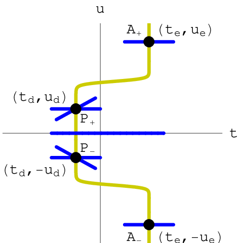
Let us first take a pair of the type points in the patch. Let us suppose that they are located at and , respectively. For simplicity, let us suppose that the spectral surfaces near the singularity point are given by
| (409) |
for a field in the representation of and two in of , where denotes the fiber coordinate of the canonical bundle in the patch, when is taken as the frame. Since the transformation maps to , the fiber coordinate near the point transforms into near the point , as we already discussed in section 3.2.4. The spectral surfaces near the point , then, should be given by
| (410) |
It follows from (166, 167) that the hypermultiplet wavefunctions in the field-theory local model around the point are given by
| (411) | |||||
| (412) | |||||
| (413) | |||||
| (414) | |||||
| (415) | |||||
| (416) |
where . Zero mode wavefunctions correspond to holomorphic sections of and , and they are expressed locally around , by taking trivialization frames of and , as
| (417) |
respectively. Near the point , the overlap form for the down-type Yukawa couplings is locally given by
| (418) | |||||
| (419) |
The form is localized near , because of the three Gaussian factors “”. Thus, the Yukawa coupling of the three zero modes in the local neighborhood of is determined by the last product of the three ’s at on the right-hand side of (419).
Similarly, the hypermultiplet wavefunctions in the field-theory local model near are given by
| (420) | |||||
| (421) | |||||
| (422) | |||||
| (423) | |||||
| (424) | |||||
| (425) |
The overlap form near becomes
| (426) | |||||
| (427) |
Suppose that the transformation is defined on the sections of line bundles and those of by
| (428) |
with that may be different for and , where is the pull-back of the coefficient function using the local trivialization frame in (417). Equivalently, for ,
| (429) |
One can then see from (411–416) and (420–425) that the zero mode wavefunctions for and for satisfy the relation
| (430) |
for all the representations, , and . The transformation on the holomorphic sections of on the matter curve and those of on the curve is now translated into a transformation between the fields of the pair of field-theory local models around and . We can also7777 77 Since the field configuration is—by definition—the zero mode wavefunction corresponding to a holomorphic section , it is not necessary to make an extra effort to show that the right-hand side is a zero mode, though. see in the language of the field theories that zero modes are mapped to zero modes by the transformation (430). This is because the transformation (430) is essentially a pull-back times , and because the background configuration is invariant under the pull-back by .
The symmetry transformation on and for matter parity must become a transformation between the pair of field-theory local models around and . The representation of has an irreducible decomposition (114) with and , and fields , , , and in an irreducible component around are mapped to those in the same irreducible component around up to transformation. The transformation (430) is not just a map from a space of zero mode wavefunctions in to itself, but it is regarded also as a map from a space of all kinds of field configuration in to itself. It is easy to see for any choice of that the transformation (430) preserves the bilinear part of the action (109, 110) of the pair of field theories, and we have already seen that the zero mode configurations around and those around are mapped to each other. However, in order for the transformation to be a symmetry between the pair of field theory local models, all the interactions in (109, 110) need to be preserved under the transformation, not just the bilinear part of (109, 110).
The down-type Yukawa couplings (418, 426) originate from trilinear interactions of the field theory on 7+1 dimensions. The transformation for matter parity should be a symmetry between the pair of the field theories, and hence it must be a symmetry between this interaction7878 78 The structure constant of should be common to both and is omitted from (418, 426). at and at . Noting that the trilinear interaction is transformed under (430) to
| (431) |
we find that we have to take in order for the transformation to be a symmetry between the pair of field theories at and .
Let us now take a pair (, ) of the -type points in the patch. We suppose that they are located at and , respectively. For simplicity, let us suppose that the spectral surfaces near the point are locally given by
| (432) |
for the fields in the representation and , respectively, of . Because of the symmetry, the spectral surfaces near the point should be given by
| (433) |
The approximate wavefunctions for the zero modes in the representation is
with the functions and determined by the discussion in the appendix C. The zero mode wavefunctions of the fields in representation, on the other hand, are of the form
| (440) | |||||
| (441) |
near the points , respectively. Under the transformation on the sections of with , the section is mapped to , and its corresponding wavefunctions are related to the original one by7979 79 The form of the matrix can be understood as follows. Let us take a trivialization of , and denote the local frame as . then becomes a local frame of , and hence of . Under the transformation (428), (442) for . At the ramification loci of , which are the -type points in this context, the rank-2 bundle can be described locally by using a frame , as we already did in appendix C. Since both and are multiplied by under the transformation, we find (443) The diagonal entries of with the opposite sign come from the opposite sign in (442, 443).
| (444) |
and
| (445) |
Therefore, the transformation on the sections of is translated to a transformation (444, 445) between the space of field configuration in the component of in the field theory local model at and the one in the local model at . The zero mode wavefunctions in the representation satisfy (430) under the transformation on , with yet to be determined. The transformation on the sections of is translated to the transformation (430) between the spaces of field configuration in the component near and .
Just like we required that the transformations on the fields in the irreducible components define a symmetry transformation between a pair of field theory local models at and , we need to require that the transformations on the fields in the and components gives a symmetry of the pair of field theory local models. The field theories contain a trilinear interaction that gives rise to the up-type Yukawa couplings. It is proportional to an overlap from
| (446) |
which contains the part of the structure constant of , but the part is omitted. One can see from (444, 445, 430) that this interaction at is mapped to the same interaction at by the transformation and vice versa, up to a multiplication constant:
| (447) |
We therefore conclude that should be chosen, in order for the transformation to be a symmetry between the pair of field theory local models at and .
References
- [1] R. Tatar and T. Watari, “Proton decay, Yukawa couplings and underlying gauge symmetry in string theory,” Nucl. Phys. B 747, 212 (2006) [arXiv:hep-th/0602238].
- [2] H. Hayashi, T. Kawano, R. Tatar and T. Watari, “Codimension-3 Singularities and Yukawa Couplings in F-theory,” arXiv:0901.4941 [hep-th].
- [3] R. Tatar, Y. Tsuchiya and T. Watari, “Right-handed Neutrinos in F-theory Compactifications,” Nucl. Phys. B 823, 1 (2009) [arXiv:0905.2289 [hep-th]].
- [4] J. L. Bourjaily, “Local Models in F-Theory and M-Theory with Three Generations,” arXiv:0901.3785 [hep-th].
- [5] J. J. Heckman, A. Tavanfar and C. Vafa, “The Point of in F-theory GUTs,” arXiv:0906.0581 [hep-th].
- [6] R. Donagi and M. Wijnholt, “Model Building with F-Theory,” arXiv:0802.2969 [hep-th].
- [7] C. Beasley, J. J. Heckman and C. Vafa, “GUTs and Exceptional Branes in F-theory - I,” JHEP 0901, 058 (2009) [arXiv:0802.3391 [hep-th]].
- [8] H. Hayashi, R. Tatar, Y. Toda, T. Watari and M. Yamazaki, “New Aspects of Heterotic–F Theory Duality,” Nucl. Phys. B 806, 224 (2009) [arXiv:0805.1057 [hep-th]].
- [9] R. Donagi and M. Wijnholt, “Higgs Bundles and UV Completion in F-Theory,” arXiv:0904.1218 [hep-th].
- [10] V. Sadov, “Generalized Green-Schwarz mechanism in F theory,” Phys. Lett. B 388, 45 (1996) [arXiv:hep-th/9606008].
- [11] D. E. Diaconescu and G. Ionesei, “Spectral covers, charged matter and bundle cohomology,” JHEP 9812, 001 (1998) [arXiv:hep-th/9811129].
- [12] M. Wijnholt, “F-Theory, GUTs and Chiral Matter,” arXiv:0809.3878 [hep-th].
- [13] R. Tatar and T. Watari, “GUT Relations from String Theory Compactifications,” Nucl. Phys. B 810, 316 (2009) [arXiv:0806.0634 [hep-th]].
- [14] S. Katz and C. Vafa, “Matter From Geometry,” Nucl. Phys. B 497, 146 (1997) [arXiv:hep-th/9606086].
- [15] version 2 of [30].
- [16] J. Marsano, N. Saulina and S. Schafer-Nameki, “Monodromies, Fluxes, and Compact Three-Generation F-theory GUTs,” JHEP 0908, 046 (2009) [arXiv:0906.4672 [hep-th]].
- [17] C. Beasley, J. J. Heckman and C. Vafa, “GUTs and Exceptional Branes in F-theory - II: Experimental Predictions,” arXiv:0806.0102 [hep-th].
- [18] R. Donagi and M. Wijnholt, “Breaking GUT Groups in F-Theory,” arXiv:0808.2223 [hep-th].
- [19] M. Kuriyama, H. Nakajima and T. Watari, “A Theoretical Framework for R-parity Violation,” Phys. Rev. D 79, 075002 (2009) [arXiv:0802.2584 [hep-ph]].
- [20] J. Marsano, N. Saulina and S. Schafer-Nameki, “F-theory Compactifications for Supersymmetric GUTs,” arXiv:0904.3932 [hep-th].
- [21] R. Blumenhagen, T. W. Grimm, B. Jurke and T. Weigand, “Global F-theory GUTs,” arXiv:0908.1784 [hep-th].
- [22] M. Bershadsky, K. A. Intriligator, S. Kachru, D. R. Morrison, V. Sadov and C. Vafa, “Geometric singularities and enhanced gauge symmetries,” Nucl. Phys. B 481, 215 (1996) [arXiv:hep-th/9605200].
- [23] A. Grassi and D. R. Morrison, “Group representations and the Euler characteristic of elliptically fibered Calabi-Yau threefolds,” arXiv:math/0005196.
- [24] G. Rajesh, “Toric geometry and F-theory/heterotic duality in four dimensions,” JHEP 9812, 018 (1998) [arXiv:hep-th/9811240].
- [25] V. Bouchard, J. J. Heckman, J. Seo and C. Vafa, “F-theory and Neutrinos: Kaluza-Klein Dilution of Flavor Hierarchy,” arXiv:0904.1419 [hep-ph].
- [26] R. Donagi, Y. H. He, B. A. Ovrut and R. Reinbacher, “The particle spectrum of heterotic compactifications,” JHEP 0412, 054 (2004) [arXiv:hep-th/0405014].
- [27] G. Curio, “Chiral matter and transitions in heterotic string models,” Phys. Lett. B 435, 39 (1998) [arXiv:hep-th/9803224].
- [28] R. Friedman, J. Morgan and E. Witten, “Vector bundles and F theory,” Commun. Math. Phys. 187 (1997) 679 [arXiv:hep-th/9701162].
- [29] R. Blumenhagen, S. Moster, R. Reinbacher and T. Weigand, “Massless spectra of three generation U(N) heterotic string vacua,” JHEP 0705, 041 (2007) [arXiv:hep-th/0612039].
- [30] J. J. Heckman and C. Vafa, “Flavor Hierarchy From F-theory,” arXiv:0811.2417 [hep-th].
- [31] R. Friedman, J. Morgan and E. Witten, “Vector Bundles over Elliptic Fibrations,” arXiv:alg-geom/9709029.
- [32] R. Donagi, B. A. Ovrut, T. Pantev and R. Reinbacher, “SU(4) Instantons on Calabi-Yau Threefolds with Fundamental Group,” JHEP 0401, 022 (2004) [arXiv:hep-th/0307273].
- [33] M. Buican, D. Malyshev, D. R. Morrison, H. Verlinde and M. Wijnholt, “D-branes at singularities, compactification, and hypercharge,” JHEP 0701, 107 (2007) [arXiv:hep-th/0610007].
- [34] T. Watari and T. Yanagida, “Product-group unification in type IIB string theory,” Phys. Rev. D 70, 036009 (2004) [arXiv:hep-ph/0402160].
- [35] R. Blumenhagen, G. Honecker and T. Weigand, “Loop-corrected compactifications of the heterotic string with line bundles,” JHEP 0506 (2005) 020 [arXiv:hep-th/0504232].
- [36] B. A. Ovrut, T. Pantev and R. Reinbacher, “Torus-fibered Calabi-Yau threefolds with non-trivial fundamental group,” JHEP 0305, 040 (2003) [arXiv:hep-th/0212221].
- [37] N. Hitchin, “The Self-duality Equations on a Riemann Surface,” Proc. London Math. Soc. (3) 55, (1987) 59-126.
- [38]
L. J. Hall, M. P. Salem and T. Watari,
“Quark and Lepton Masses from Gaussian Landscapes,”
Phys. Rev. Lett. 100, 141801 (2008)
[arXiv:0707.3444 [hep-ph]];
“Statistical Understanding of Quark and Lepton Masses in Gaussian Landscapes,” Phys. Rev. D 76, 093001 (2007) [arXiv:0707.3446 [hep-ph]]. - [39] N. Arkani-Hamed and M. Schmaltz, “Hierarchies without symmetries from extra dimensions,” Phys. Rev. D 61, 033005 (2000) [arXiv:hep-ph/9903417].
- [40] D. Cremades, L. E. Ibanez and F. Marchesano, “Computing Yukawa couplings from magnetized extra dimensions,” JHEP 0405, 079 (2004) [arXiv:hep-th/0404229].
- [41] P. Griffiths and J. Harris, “Principles of algebraic geometry,” Wiley (1994)
- [42] L. J. Hall, H. Murayama and N. Weiner, “Neutrino mass anarchy,” Phys. Rev. Lett. 84, 2572 (2000) [arXiv:hep-ph/9911341]; N. Haba and H. Murayama, “Anarchy and hierarchy,” Phys. Rev. D 63, 053010 (2001) [arXiv:hep-ph/0009174].
- [43] L. J. Hall, M. P. Salem and T. Watari, “Neutrino mixing and mass hierarchy in Gaussian landscapes,” Phys. Rev. D 79, 025010 (2009) [arXiv:0810.2561 [hep-th]].
- [44] L. Randall and D. Simmons-Duffin, “Quark and Lepton Flavor Physics from F-Theory,” arXiv:0904.1584 [hep-ph].
- [45] S. Katz and D. R. Morrison, “ Gorenstein Threefold Singularities with Small Resolutions via Invariant Theory for Weyl Groups,” J. Alg. Geom. 1 (1992) 449–530 [arXiv:alg-geom/9202002].
- [46] N. Hitchin, “Stable Bundles and Integrable Systems,” Duke Math. J. 54 (1987) 91.
- [47] R. Y. Donagi and D. Gaitsgory, “The gerbe of Higgs bundles,” Transform. Groups 7 (2002) 109 [arXiv:math/0005132].
- [48] S. Cecotti, M. C. N. Cheng, J. J. Heckman and C. Vafa, “Yukawa Couplings in F-theory and Non-Commutative Geometry,” arXiv:0910.0477 [hep-th].
- [49] J. P. Conlon and E. Palti, “Aspects of Flavour and Supersymmetry in F-theory GUTs,” arXiv:0910.2413 [hep-th].