Centrifugally induced curvature drift instability in AGN

For studying AGN winds the fundamental problem relates to the understanding of a question: how the plasma goes through the Light Cylinder Surface (LCS), which is the hypothetical zone where the linear velocity of rotation equals the speed of light. This implies that the plasma particles, which move along quasi-straight magnetic field lines in the nearby area of the LCS, must reach the speed of light. Generally speaking no physical system can maintain such a motion and a certain twisting process of the magnetic field lines must operate on the LCS. On the other hand if the trajectories are given by the Archimedes spiral, then the particles can cross the LCS avoiding the light cylinder problem [1]. An additional step in this investigation is to identify the appropriate mechanism that provides the twisting of the magnetic field lines, giving rise to the shape of the Archimedes spiral, and in turn insures that the dynamics is force-free.

Since the innermost region of AGNs rotates, the role of the Centrifugal Force (CF) appears interesting. The centrifugally driven outflows have been extensively studied. Generalizing the work developed in [2] it was shown that due to the centrifugal acceleration, electrons gain very high energies with Lorentz factors up to $\gamma\sim 10^{8}$ [3, 4]. This implies that the energy budget in the AGN winds is very high.

The centrifugally driven parametric instability was first introduced in [5, 6] for the Crab pulsar and AGN jets respectively. Another kind of the instability which might be induced by the CF is the so called Curvature Drift Instability (CDI). In [7] the two-component relativistic plasma has been considered to study the role of the centrifugal acceleration in the curvature drift instability for pulsar magnetospheres. The investigation demonstrated high efficiency of the CDI. To investigate the twisting process of magnetic field lines due to the CDI, we apply the method developed in [7, 8] to AGN winds.

The paper is arranged as follows. In Sect. 2, we introduce the curvature drift waves and derive the dispersion relation. In Sect. 3, the results for typical AGNs are presented and, in Sect. 4, we summarize our results.

We begin our investigation by considering the two-component plasma consisting of the relativistic electrons with the Lorentz factor $\gamma_{e}\sim 10^{5-8}$ (see [3, 4]) and the bulk component (protons) with $\gamma_{b}\sim 10$. Since we are interested in the twisting process, we suppose that initially the field lines are almost rectilinear to study how this configuration changes in time.

We express the equation of motion in the cylindrical coordinates (see Fig. 1) and we start by considering the Euler equation:

the continuity equation:

and the induction equation:

where $\alpha=\{e,b\}$, $\xi\equiv\sqrt{1-\Omega^{2}R^{2}/c^{2}},$, ${\bf p_{\alpha}}$ is the momentum, ${\bf v_{\alpha}}$ - the velocity and ${\gamma_{\alpha}}$ is the Lorentz factor of the relativistic particles.

We linearize the system of equations Eqs. (1-3), perturbing all physical quantities around the leading state $\Psi\approx\Psi^{0}+\Psi^{1}$, where $\Psi=\{n,{\bf v},{\bf p},{\bf E},{\bf B}\}$ and $\Psi^{1}(t,{\bf r})\propto\Psi^{1}(t)\exp\left[i\left({\bf kr}\right)\right]$.

Then, from Eqs. (1-3) we derive the linearized set of equations governing the CDI:

By $u_{\alpha}=\gamma_{\alpha_{0}}v_{{}_{\parallel}}^{2}/(\omega_{B}R_{B})$, we denote the curvature drift velocity along the $x$ axis, where $\omega_{\alpha B}=q_{\alpha}B_{0}/m_{\alpha}c$, $R_{B}$ is the curvature radius of magnetic field lines, $v_{{}_{\parallel}}\approx c\cos(\Omega t)$, $B_{0}=\sqrt{2L/(R_{lc}c^{2})}$, $L$ is the luminosity of the AGN and $R_{lc}=c/\Omega$ - the light cylinder radius. In deriving Eqs. (4-6), the wave propagating almost perpendicular to the equatorial plane, was considered and the expression $v^{1}_{r}\approx cE^{1}_{x}/B_{0}$ was taken into account. For simplicity, the set of equations are given in terms of the coordinates of the field line (see Fig. 1).

We express $v^{1}_{\alpha x}$ and $n^{1}_{\alpha}$ in the following way:

where

Then, by substituting Eqs. (7) and (8) into Eqs. (4-6), it becomes straightforward to solve the system for the toroidal component and find a corresponding increment of the instability:

We investigate the CDI growth rate in terms of the wavelength, the density of relativistic electrons, their Lorentz factors and the AGN bolometric luminosity.

In studying the behaviour of the instability as a function of the wavelength, we examine the typical AGN parameters: $M_{BH}=10^{8}\times M_{\odot}$, $\Omega=5\times 10^{-5}s^{-1}$ and $L=10^{44}erg/s$, where $M_{BH}$ is the AGN mass, $M_{\odot}$ is the solar mass and $L$ is the bolometric luminosity of the AGN.

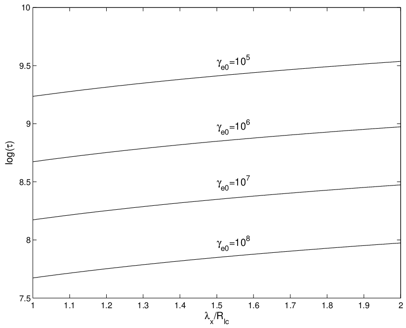
We consider Eq. (11) and plot the logarithm of the instability timescale $\tau\equiv 1/\Gamma$ versus the wavelength. The present consideration is based on the centrifugal acceleration. As shown in [3], due to the CF, the relativistic particles can reach very high Lorentz factors. For this purpose, it is reasonable to investigate the efficiency of the instability in terms of the wavelength but for different values of Lorentz factors. Fig. 2 shows the mentioned behaviour for different parameters. Different curves correspond to different values of Lorentz factors. For the given range of $\lambda_{x}$ and different values of $\gamma_{e0}$, the CDI time scale varies from $\sim 10^{7}s$ ($\lambda_{x}/R_{lc}=1$, $\gamma_{e0}=10^{8}$) to $\sim 10^{9}$ ($\lambda_{x}/R_{lc}=2$, $\gamma_{e0}=10^{5}$).

In Fig. 3 the plots of $log(\tau)$ versus the AGN wind density illustrate that the timescale is a continuously decreasing function of $n_{e0}/n_{m}$. As we see from the figure, $\tau$ varies from $\sim 10^{9}s$ ($n_{e0}/n_{m}=0.001$, $\gamma_{e0}=10^{5}$) to $\sim 10^{6}s$ ($n_{e0}/n_{m}=1$, $\gamma_{e0}=10^{8}$).

In Fig. 4, the plot of $log(\tau)$ versus $log(\gamma_{e0})$ is shown for different luminosities. As we see, the instability timescale varies from $\sim 10^{10}s$ ($\gamma_{e0}=10^{5}$, $L/L_{E}=1$) to $\sim 10^{8}s$ ($\gamma_{e0}=10^{7}$, $L/L_{E}=0.01$). On the other hand, the plots for different luminosities illustrate another property of $\tau$: by increasing the luminosity of the AGN, the corresponding instability becomes less efficient.

To observe this particular feature more clearly, we consider how in Fig. 5 the dependence of $log(\tau)$ on $L/L_{E}$ is clearly evident for different values of densities. From the plots, it is seen that by increasing the luminosity, the timescale continuously increases. For the afore mentioned area of quantities, the timescale varies from $\sim 10^{7}s$ ($L/L_{E}=0.01$, $n_{e0}/n_{J}=1$) to $\sim 10^{10}s$ ($L/L_{E}=1$, $n_{e0}/n_{J}=0.001$).

We observe from the present investigation that the instability timescale varies in the following range: $\tau\in\{10^{6};10^{10}\}s$. To specify how efficient the CDI is, it is pertinent to examine an accretion process, estimate its corresponding evolution timescale, and compare this value with that of the CDI.

Considering the problem of fuelling AGNs [9] it was showed that the accretion timescale can be estimated by the following form $t_{evol}=3.53\times 10^{13}\left(10L/L_{E}\right)^{-22/27}\left(10^{-8}M_{BH}/M_{\odot}\right)^{-4/27}s$. As is clear from this formula, the accretion evolution timescale depends on two major AGN parameters, the luminosity ($L$) and the AGN mass ($M_{BH}$). Therefore, it is reasonable to investigate $t_{evol}$ versus $L$ and $M_{BH}$. Let us examine the following ranges of variables: $M_{9}\equiv M_{BH}/(10^{9}\times M_{\odot})\in\{0.01;1\}$ and $L/L_{E}\in\{0.01;1\}$. Then it is easy to show that the minimum value of the evolution timescale is of the order of $\sim 10^{12}s$, which corresponds to $M_{9}=1$ and $L/L_{E}=1$, whereas the maximum value, approximately $\sim 10^{15}s$, corresponds to the following pair of variables $M_{9}=0.001$ and $L/L_{E}=0.01$.

As has been found, $\tau$ varies in the range $\sim(10^{6}-10^{10})s$, whereas the sensible area of $t_{evol}$ is $\sim(10^{12}-10^{15})s$. Therefore, the instability timescale is less than the evolution timescale of the accretion by many orders of magnitude, which implies that the linear stage of the CDI is extremely efficient.

The twisting process of magnetic field lines requires a certain amount of energy and it is natural to study the energy budget of this process. For this reason we have to introduce the maximum of the possible luminosity $L_{max}=\dot{M}c^{2}$ and compare this with the ”luminosity” corresponding to the reconstruction of the magnetic field configuration $L_{m}\equiv\Delta E_{m}/\Delta t\approx\Delta E_{m}/\tau$, where $\Delta E_{m}$ is the variation in the magnetic energy due to the curvature drift instability.

We consider a AGN of the luminosity, $L=10^{45}erg/s$, then, the accretion provides the following maximum value: $L_{max}=L/0.1=10^{46}erg/s$. On the other hand, if the process of sweepback is realistic, the magnetic ”luminosity” cannot exceed $L_{max}$. The magnetic ”luminosity” can be expressed by following $L_{m}=B_{r}^{2}R_{lc}^{3}\kappa/(4\pi\tau)$, with $B_{r}=B_{r}^{0}exp(t/\tau)$, where $B_{r}^{0}$ is the initial perturbation of the toroidal component of magnetic field and $\kappa\equiv\Delta R/R_{lc}<<1$ represents the non-dimensional thickness of a thin spatial layer close to the LCS.

We introduce the initial non-dimensional perturbation, $\delta$, defined to be $\delta\equiv B_{r}^{0}/B_{0}$, where by $B_{0}$ we denote the induction of the magnetic field in the leading state. By considering the following set of parameters $\gamma_{e0}=\{10^{5};10^{6};10^{7};10^{8}\}$, $R_{B}\approx R_{lc}$, $n_{e0}=0.001cm^{-3}$, $\lambda_{\phi}=100R_{lc}$, $\lambda_{x}=R_{lc}$ and $L=10^{45}erg/s$, we investigate the behaviour of $L_{m}/L_{max}$ versus the initial perturbation for the characteristic timescale ($t\approx\tau$). One can see that, $L_{m}/L_{max}$ varies from $\sim 0$ ($\delta=0$) to $\sim 2.3\times 10^{-9}$ ($\delta=0.1$, $\gamma_{e0}=10^{8}$). Therefore, $L_{max}>>L_{m}$ which means that only a tiny fraction of the total energy goes to the sweepback, making this process feasible.

We summarize the principal steps and conclusions of our study to be:

1. 1.

   Considering the relativistic two-component plasma for AGN winds, the centrifugally driven curvature drift instability has been studied.

2. 2.

   Taking into account a quasi single approach for the particle dynamics, we linearized the Euler continuity and induction equations. The dispersion relation characterizing the parametric instability of the toroidal component of the magnetic field has been derived.

3. 3.

   By considering the proper frequency of the curvature drift modes, the corresponding expression of the instability increment has been obtained for the light cylinder region.

4. 4.

   The efficiency of the CDI has been investigated by adopting four physical parameters, namely: the wavelength, flow density and Lorentz factors of electrons, and the luminosity of AGNs.

5. 5.

   By considering the evolution process of accretion, the corresponding timescale has been estimated for a physically reasonable area in the parametric space $L-M_{BH}$. It was shown that the instability timescale was lower by many orders of magnitude than the evolution timescale, indicating extremely high efficiency of the CDI.

6. 6.

   Examining the instability from the point of view of the energy budget, we have seen that the sweepback of the magnetic field lines requires only a small fraction of the total energy, which means that the CDI is a realistic process.

References

- (1) Rogava A. D., Dalakishvili G. & Osmanov Z., 2003, Gen. Rel. and Grav., 35, 1133
- (2) Gangadhara R.T., Lesch H. 1997, A&A, 323, L45
- (3) Osmanov Z., Rogava A.S. & Bodo G., 2007, ApJ, 470, 395
- (4) Rieger F. M. & Aharonian F. A., 2008, A&A, 479, 5
- (5) Machabeli G., Osmanov Z. & Mahajan S., 2005, Phys. Plasmas, 12, 062901
- (6) Osmanov Z., 2008, Phys. Plasmas, 15, 032901
- (7) Osmanov Z., Dalakishvili Z. & Machabeli Z. 2008, MNRAS, 383, 1007
- (8) Osmanov Z., Shapakdze D. & Machabeli G., 2008, MNRAS, (submitted)
- (9) King A. R. & Pringle J. E., 2007, MNRAS, 377, 25