TTP09-38 arXiv:0910.2663
SFB/CPP-09-94 October 2009
Lepton flavour violation in the MSSM

Jennifer Girrbach¹ Susanne Mertens^1,2 Ulrich Nierste¹ and Sören Wiesenfeldt^1,3
¹ Institut für Theoretische Teilchenphysik, Karlsruhe Institute of Technology, Universität Karlsruhe, 76128 Karlsruhe, Germany
² Institut für Experimentelle Kernphysik, Karlsruhe Institute of Technology, Universität Karlsruhe, 76128 Karlsruhe, Germany
³ Helmholtz Association, Anna-Louisa-Karsch-Straße 2, 10178 Berlin, Germany

Abstract

We derive new constraints on the quantities $\delta_{XY}^{ij}$ , $X,Y=L,R$ , which parametrise the flavour-off-diagonal terms of the charged slepton mass matrix in the MSSM. Considering mass and anomalous magnetic moment of the electron we obtain the bound $|\delta^{13}_{LL}\delta^{13}_{RR}|\stackrel{{\scriptstyle<}}{{{}_{\sim}}}0.1$ for $\tan\beta=50$ , which involves the poorly constrained element $\delta^{13}_{RR}$ . We improve the predictions for the decays $\tau\to\mu\gamma$ , $\tau\to e\gamma$ and $\mu\to e\gamma$ by including two-loop corrections which are enhanced if $\tan\beta$ is large. The finite renormalisation of the PMNS matrix from soft SUSY-breaking terms is derived and applied to the charged-Higgs-lepton vertex. We find that the experimental bound on $BR(\tau\to e\gamma)$ severely limits the size of the MSSM loop correction to the PMNS element $U_{e3}$ , which is important for the proper interpretation of a future $U_{e3}$ measurement. Subsequently we confront our new values for $\delta^{ij}_{LL}$ with a GUT analysis. Further, we include the effects of dimension-5 Yukawa terms, which are needed to fix the Yukawa unification of the first two generations. If universal supersymmetry breaking occurs above the GUT scale, we find the flavour structure of the dimension-5 Yukawa couplings tightly constrained by $\mu\to e\gamma$ .

Abstract

1 Introduction

Weak-scale supersymmetry (SUSY) is an attractive framework for physics beyond the standard model (SM) of particle physics. The SM fields are promoted to superfields, with additional constituents of opposite spin. Due to their identical couplings, they cancel the quadratic divergent corrections to the Higgs mass. Since none of the SUSY partners have been observed in experiments, supersymmetry must be broken and the masses of the SUSY partners are expected to be in the multi-GeV region.

A supersymmetric version of the standard model requires a second Higgs doublet in order to cancel the Higgsino-related anomalies and to achieve electroweak symmetry breaking. At tree level, one of the Higgs doublets, $H_{u}$ , couples to the up-type particles, whereas the other doublet, $H_{d}$ , couples to the down type particles. The Yukawa couplings of the minimal supersymmetric standard model (MSSM) read


	$\displaystyle W_{\text{MSSM}}$	$\displaystyle=Y_{u}^{ij}u^{c}_{i}Q_{j}H_{u}+Y_{d}^{ij}d^{c}_{i}Q_{j}H_{d}+Y_{l}^{ij}e^{c}_{i}L_{j}H_{d}+\mu H_{d}H_{u}\,.$	(1a)
Neutrinos are massless in the MSSM; however, experiments and cosmological observations consistently point at small but non-vanishing masses in the sub-eV region. We will therefore consider an extended MSSM with three right handed neutrinos, where the Yukawa couplings are given by
	$\displaystyle W$	$\displaystyle=W_{\text{MSSM}}+Y_{\nu}^{ij}\nu^{c}_{i}L_{j}H_{u}+\frac{1}{2}M_{R}^{ij}\nu^{c}_{i}\nu^{c}_{j}\,.$	(1b)

Here, $Q$ and $L$ denote the chiral superfields of the quark and lepton doublets and $u^{c}$ , $d^{c}$ , $e^{c}$ and $\nu^{c}$ the up and down-quark, electron and neutrino singlets, respectively. Each chiral superfield consists of a fermion and its scalar partner, the sfermion. The Yukawa coupling matrices $Y_{u,d,l,\nu}$ are defined with the right-left (RL) convention. The field $\nu^{c}$ is sterile under the SM group, so we allow for a Majorana mass term in addition to the Dirac coupling. The respective mass matrix is denoted by $M_{R}$ and the scale of $M_{R}$ is undetermined but expected to be above the electroweak scale, $M_{\text{ew}}$ (see Sec. 4).

The Higgs fields acquire the vacuum expectation values (vevs)

\displaystyle\langle H_{u}\rangle

\displaystyle=v_{u}\,,\mspace{60mu}\langle H_{d}\rangle=v_{d}\,.

(2)

where $|v_{u}|^{2}+|v_{d}|^{2}=v^{2}=(174\ \text{GeV})^{2}$ . The ratio of the two vevs is undetermined and defines the parameter $\tan\beta$ ,

\displaystyle\frac{v_{u}}{v_{d}}=:\tan\beta\ .

(3)

While $\tan\beta$ is a free parameter of the theory, there exist lower and upper bounds on its value. Experimentally, Higgs searches at LEP rule out the low- $\tan\beta$ region in simple SUSY models [1]. This result fits nicely with the theoretical expectation that the top Yukawa coupling should not be larger than one. The region of the MSSM parameter space with large values of $\tan\beta$ is of special importance for the flavour physics of quarks and leptons. We therefore have a brief critical look at the upper bounds on this parameter: Demanding a perturbative bottom Yukawa coupling $y_{b}$ naïvely leads to an upper limit on $\tan\beta$ of about 50 inferred from the tree-level relation

\displaystyle y_{b}=-\frac{m_{b}}{v\cdot\cos\beta}\approx-\frac{m_{b}}{v}\tan\beta\ .

(4)

Similarly, the MSSM provides a natural radiative breaking mechanism of the electroweak symmetry as long as $y_{b}<y_{t}$ at a low scale [2]. At tree level, the ratio of the Yukawa couplings is given by

\displaystyle 1>\left|\frac{y_{b}}{y_{t}}\right|=\frac{m_{b}}{m_{t}}\tan\beta\;.

(5)

Since $m_{t}(\mu)/m_{b}(\mu)\approx 60$ at the electroweak scale, $\tan\beta$ should not exceed this value.

Both arguments, however, do only hold at tree level. In particular, down quarks as well as charged leptons couple to $H_{u}$ via loops. As a result, if we take $\tan\beta$ -enhanced contributions into account, an explicit mass renormalisation changes the relation of Yukawa coupling and mass [3, 4, 5]. The $\tan\beta$ enhancement of the bottom coupling in Eq. (4) can be compensated; similarly, the ratio of the Yukawa couplings is changed due to an explicit bottom quark mass renormalisation. We will find that values of $\tan\beta$ up to 100 both provide small enough Yukawa couplings and do not destroy natural electroweak symmetry breaking.

Large values for $\tan\beta$ are interesting for two reasons. One, in various grand-unified theories (GUTs), top and bottom Yukawa couplings are unified at a high scale. In this case, it is natural to expect $\tan\beta=m_{t}/m_{b}$ , as shown above. Two, many supersymmetric loop processes are $\tan\beta$ -enhanced due to chirality-flipping loop processes with supersymmetric particles in the loop. This enhancement can compensate the loop suppression and therefore large values of $\tan\beta$ lead to significant SUSY corrections.

In this paper, we will study the lepton sector in the (extended) MSSM. Since the neutrinos are massive, the leptonic mixing matrix, $U_{\text{PMNS}}$ , is no longer trivial and leads to lepton flavour violation (LFV). In its standard parametrisation, it reads

\displaystyle U_{\text{PMNS}}

\displaystyle=\begin{pmatrix}1&0&0\cr 0&c_{23}&s_{23}\cr 0&-s_{23}&c_{23}\end{pmatrix}\begin{pmatrix}c_{13}&0&s_{13}e^{i\delta}\cr 0&1&0\cr-s_{13}e^{i\delta}&0&c_{13}\end{pmatrix}\begin{pmatrix}c_{12}&s_{12}&0\cr-s_{12}&c_{12}&0\cr 0&0&1\end{pmatrix}\begin{pmatrix}e^{i\frac{\alpha_{1}}{2}}&0&0\cr 0&e^{i\frac{\alpha_{2}}{2}}&0\cr 0&0&1\end{pmatrix},

(6)

with $s_{ij}=\sin\theta_{ij}$ and $c_{ij}=\cos\theta_{ij}$ . The two phases $\alpha_{1,2}$ appear if neutrinos are Majorana particles. They are only measurable in processes which uncover the Majorana nature of neutrinos, such as neutrinoless double beta decay.

The PMNS matrix allows for flavour transitions in the lepton sector, in particular neutrino oscillations, through which its parameters are well constrained. Compared with the mixing angles of the quark mixing matrix, $V_{\text{CKM}}$ , two mixing angles, namely the atmospheric and solar mixing angles, $\theta_{23}=\theta_{\text{atm}}$ and $\theta_{12}=\theta_{\text{sol}}$ , are surprisingly large, whereas the third mixing angle is small. The current experimental status at $1\sigma$ level is as follows [6]:¹¹ 1 Recently, a hint for non-zero $\theta_{13}$ , $\sin^{2}{\theta_{13}}=0.016\pm 0.010\ (1\sigma)$ , was claimed in Ref. [7].

$\displaystyle\theta_{12}$	$\displaystyle=34.5\pm 1.4\;,$	$\displaystyle\Delta m_{21}^{2}$	$\displaystyle=7.67^{+0.22}_{-0.21}\cdot 10^{-5}\ \textrm{eV}^{2},$
$\displaystyle\theta_{23}$	$\displaystyle=42.3^{+5.1}_{-3.3}\;,$	$\displaystyle\Delta m_{31}^{2}$	$\displaystyle=\begin{cases}-2.37\pm 0.15\cdot 10^{-3}\ \textrm{eV}^{2}&\textrm{inverted hierarchy},\\ +2.46\pm 0.15\cdot 10^{-3}\ \textrm{eV}^{2}&\textrm{normal hierarchy},\end{cases}$
$\displaystyle\theta_{13}$	$\displaystyle=0.0^{+7.9}_{-0.0}\;.$			(7)

These values are determined by the atmospheric and solar mass splitting $\Delta m_{\text{atm}}^{2}=\Delta m_{13}^{2}$ , $\Delta m_{\text{sol}}^{2}=\Delta m_{21}^{2}$ , leaving the absolute mass scale open. The pattern of mixing angles is close to tri-bimaximal, corresponding to $\theta_{23}=45^{\circ}$ , $\theta_{12}\simeq 35^{\circ}$ , and $\theta_{13}=0^{\circ}$ [8]. Due to the smallness of $\theta_{13}$ , the CP phase $\delta$ is unconstrained. Tri-bimaximal mixing can be motivated by symmetries (see Ref. [9] and references therein), which constrain fundamental quantities like Yukawa couplings or soft SUSY-breaking terms. Measurable quantities like $U_{e3}$ usually do not point directly to fundamental parameters, but are sensitive to corrections from all sectors of the theory. The analysis of such corrections is therefore worthwhile. A large portion of this paper is devoted to the influence of supersymmetric loops and higher-dimensional Yukawa terms on observables in the lepton sector of the MSSM.

In a supersymmetric framework, additional lepton flavour violation can be induced by off-diagonal entries in the slepton mass matrix, which parametrise the lepton-slepton misalignment in a model independent way. However, a generic structure of the soft masses is already excluded because too large decay rates for $l_{j}\rightarrow l_{i}\gamma$ would arise. To avoid this flavour problem, the SUSY breaking mechanism is often assumed to be flavour blind, yielding universal soft masses at a high scale. Then the PMNS matrix is the only source of flavour violation in the lepton sector, as is the CKM matrix for the quarks; this ansatz is called minimal flavour violation. The soft terms do not cause additional flavour violation and the various mass and coupling matrices are flavour-diagonal at some scale in the basis of fermion mass eigenstates, e.g.,

\displaystyle m_{\tilde{L}}^{2}=m_{\tilde{e}}^{2}

\displaystyle=m_{0}^{2}\,\mathds{1}\,,

\displaystyle m_{H_{u}}^{2}=m_{H_{d}}^{2}

\displaystyle=m_{0}^{2}\;,

\displaystyle A_{l}

\displaystyle=A_{0}Y_{l}\;.

(8)

Here, $m_{\tilde{L},\tilde{e}}^{2}$ denote the soft mass matrices of the sleptons (see Eq. (87)), $m_{H}^{2}$ the analogous soft masses of the Higgs doublets, and $A_{l}$ is the trilinear coupling matrix of the leptons.

Even if the soft terms are universal at the high scale, renormalisation group equations (RGE) can induce non vanishing off-diagonal entries in the slepton mass matrix at the electroweak scale. Lepton flavour violation can be parametrised by non-vanishing $\delta_{XY}^{ij}$ at the electroweak scale in a model-independent way, where $\delta_{XY}^{ij}$ is defined as the ratio of the flavor-violating elements of the slepton mass matrix (87) and an average slepton mass (see Eq. (16)),

\displaystyle\delta_{XY}^{ij}=\frac{\Delta m_{XY}^{ij}}{\sqrt{m_{i_{X}}^{2}m_{j_{Y}}^{2}}},\mspace{60mu}X,\,Y=L,\,R,\qquad i,\,j=1,\,2,\,3\quad(i\not=j)\ .

(9)

The flavour-off-diagonal elements $\Delta m_{XY}^{ij}$ are defined in a weak basis in which the lepton Yukawa matrix $Y_{l}$ in Eq. (1a) is diagonal. According to the chiralities of the sfermion involved, there are four different types, $\delta_{LL}$ , $\delta_{RR}$ , $\delta_{LR}$ , and $\delta_{RL}$ . The tolerated deviation from alignment can be quantified by upper bounds on $\delta_{XY}^{ij}$ , as discussed above and are already extensively studied in the literature (see for example [10, 11, 12] and references therein).

Being generically small, the sfermion propagator can be expanded in terms of these off-diagonal elements, corresponding to the mass insertion approximation (MIA) [13, 14]. Instead of diagonalising the full slepton mass matrix and dealing with mass eigenstates and rotation matrices at the vertices, in MIA one faces flavour-diagonal couplings and LFV appears as a mass insertion in the slepton propagator. This approach is valid as long as $\left|\delta_{XY}^{ij}\right|\ll 1$ and makes it possible to identify certain contributions easily. For a numerical analysis an exact diagonalisation of all mass matrices is, of course, possible. In Ref. [12] a systematic comparison between the full computation and the MIA both in the slepton and chargino/neutralino sector clarifies the applicability of these approximations.

This paper provides a comprehensive analysis of the lepton sector in the MSSM, focusing on the phenomenological constraints on the parameters $\delta_{XY}^{ij}$ in Eq. (9). In Sec. 2 we briefly review the supersymmetric threshold corrections to $y_{b}$ in Eq. (4) and relax the usually quoted upper bounds on $\tan\beta$ . In Sec. 3 we derive new constraints on the $\delta_{XY}^{ij}$ ’s by studying loop corrections to the electron mass, finite renormalisations of the PMNS matrix and the magnetic moment of the electron at large $\tan\beta$ . As a byproduct we identify all $\tan\beta$ -enhanced corrections to the charged-Higgs coupling to leptons. We then improve the MSSM predictions for the decay rates of $l_{j}\to l_{i}\gamma$ by including $\tan\beta$ -enhanced two-loop corrections. In Sec. 4 we embed the MSSM into SO(10) GUT scenarios and study RGE effects. Even for flavour-universal soft breaking terms at the GUT scale $M_{\text{GUT}}$ sizable flavour violation can be generated between $M_{\text{GUT}}$ and the mass scales of the right-handed neutrinos [15]. Comparing the results to the upper bounds on $|\delta_{XY}^{ij}|$ found in Sec. 3 enables us to draw general conclusions on GUT scenarios. We include corrections to the Yukawa couplings from dimension-5 terms and constrain their possible flavour misalignment with the dimension-4 Yukawa matrices. In Sec. 5 we summarise our results. Our notations and conventions are listed in three appendices.

2 Upper bound for $\tan\beta$

The tree level mass of a particle receives corrections due to virtual processes. Supersymmetric loop corrections are small unless a large value for $\tan\beta$ compensates for the loop suppression. We will therefore start with a discussion of $\tan\beta$ -enhanced loops and derive a relation between Yukawa coupling and mass, coming from the resummation of $\tan\beta$ -enhanced corrections to the mass to all orders.

Corrections to the mass with more than one loop and more than one coupling to Higgs fields do not produce further factors of $\tan\beta$ . Nevertheless, $\tan\beta$ -enhanced loops can become important in an explicit mass renormalisation, where $\tan\beta$ -enhanced contributions to all orders are taken into account, because counterterms are themselves $\tan\beta$ -enhanced.

Down-quarks and charged leptons receive $\tan\beta$ -enhanced corrections to their masses, due to loops with $H_{u}$ . As a coupling to $H_{u}$ does not exist at tree level, $\tan\beta$ -enhanced loops are finite; there is no counterterm to this loop induced coupling. Moreover, $\tan\beta$ -enhanced contributions to self-energies do not decouple. The coupling of $H_{u}$ to the charged slepton is proportional to $\mu$ with $\mu=\mathcal{O}(M_{\text{SUSY}})$ . On the other hand, the integration over the loop momentum gives a factor $1/M_{\text{SUSY}}$ . Thus the dependence on the SUSY mass scale cancels out. In the large $\tan\beta$ regime, neutralino-slepton and chargino-sneutrino loops can significantly change the relation between the Yukawa couplings and masses [16, 17, 18],

\displaystyle m^{(0)}_{l}=m^{\text{phys}}_{l}+\sum_{n=1}^{\infty}\left(-\Delta\right)^{n}m^{\text{phys}}_{l}=\frac{m^{\text{phys}}_{l}}{1+\Delta_{l}}\ ,

(10)

where the corrections $\Delta_{l}$ are related to the self-energy $\Sigma_{l}$ as $\Delta_{l}=-\Sigma_{l}/m_{l}$ . This relation includes all $\tan\beta$ -enhanced contributions and can be determined by only calculating two diagrams, according to chargino-sneutrino and neutralino-slepton loops (Figure 1). As a result, the relation between Yukawa coupling and physical mass is given by

\displaystyle y_{l}=-\frac{m^{(0)}_{l}}{v_{d}}=-\frac{m^{\text{phys}}_{l}}{v_{d}\left(1+\Delta_{l}\right)}\ .

(11)

Figure 1: Contribution to the self-energy

\Sigma

arising from chargino-sneutrino and neutralino-slepton loops

The individual contributions from the two diagrams to the self-energy $\Sigma=\Sigma^{\tilde{\chi}^{\pm}}+\Sigma^{\tilde{\chi}^{0}}$ are

	$\displaystyle\Sigma_{l_{L}-l_{R}}^{\tilde{\chi}^{\pm}}$	$\displaystyle=\frac{1}{16\pi^{2}}\sum_{j=1,2}M_{\tilde{\chi}_{j}^{\pm}}\,P_{L}\,\Gamma_{l}^{\tilde{\chi}_{j}^{\pm}\tilde{\nu}_{l}*}\Gamma_{l}^{\tilde{\chi}_{j}^{\pm}\tilde{\nu}_{l}}P_{L}\,B_{0}\left(M_{\tilde{\chi}_{j}^{\pm}}^{2},\,m_{\tilde{\nu}_{l}}^{2}\right),$
	$\displaystyle\Sigma_{l_{L}-l_{R}}^{\tilde{\chi}^{0}}$	$\displaystyle=\frac{1}{16\pi^{2}}\sum_{i=1,2}\sum_{j=1}^{4}M_{\tilde{\chi}_{j}^{0}}\,P_{L}\,\Gamma_{l}^{\tilde{\chi}_{j}^{0}\tilde{l}_{i}*}\Gamma_{l}^{\tilde{\chi}_{j}^{0}\tilde{l}_{i}}P_{L}\,B_{0}\left(M_{\tilde{\chi}_{j}^{0}}^{2},\,m_{\tilde{l}_{i}}^{2}\right).$		(12)

The loop integrals, couplings and rotation matrices are defined in the appendices A and B; $M_{\tilde{\chi}^{\pm}}$ and $M_{\tilde{\chi}^{0}}$ denote the chargino and neutralino masses, respectively. The $\tan\beta$ -enhanced transitions require a chirality flip and are given by

	$\displaystyle\Delta_{l}=-\frac{\Sigma_{l}}{m_{l}}=\epsilon_{l}\tan\beta$	$\displaystyle=\frac{\alpha_{1}}{4\pi}M_{1}\,\mu\,\tan\beta\left[\frac{1}{2}f_{1}\left(M_{1}^{2},\,\mu^{2},\,m_{\tilde{l}_{L}}^{2}\right)-f_{1}\left(M_{1}^{2},\,\mu^{2},\,m_{\tilde{l}_{R}}^{2}\right)+f_{1}\left(M_{1}^{2},\,m_{\tilde{l}_{L}}^{2},\,m_{\tilde{l}_{R}}^{2}\right)\right]$
		$\displaystyle\quad-\frac{\alpha_{2}}{4\pi}M_{2}\,\mu\,\tan\beta\left[\frac{1}{2}f_{1}\left(M_{2}^{2},\,\mu^{2},\,m_{\tilde{l}_{L}}^{2}\right)+f_{1}\left(M_{2}^{2},\,\mu^{2},\,m_{\tilde{\nu}_{l}}^{2}\right)\right],$		(13)

with the loop-function $f_{1}(x,y,z)$ defined in Eq. (74).

The improved relation between the Yukawa coupling and the physical mass (11) relaxes the upper bound for $\tan\beta$ , as indicated in the Introduction. Equation (4) changes to [16]

\displaystyle y_{b}

\displaystyle=-\frac{m_{b}}{v}\frac{\tan\beta}{1+\epsilon_{b}\tan\beta}\,.

(14)

For down-quarks, the SUSY contributions are dominated by gluino loops such that

\displaystyle\epsilon_{b}

\displaystyle\simeq\frac{2\alpha_{s}}{3\pi}m_{\tilde{g}}\,\mu\,f_{1}\left(m_{\tilde{b}_{1}},\,m_{\tilde{b}_{2}},\,m_{\tilde{g}}\right).

(15)

A typical value is $\epsilon_{b}\approx 0.008$ , leading to $y_{b}=\mathcal{O}(1)$ for $\tan\beta\approx 100$ (see Fig. 2). Similarly, the bound for natural electroweak symmetry breaking shifts to $\tan\beta\lesssim 100$ .

Refer to caption — Figure 2: Bottom quark coupling as a function of $\tan\beta$ for $\epsilon_{b}=0$ (black-dashed) and $\epsilon_{b}=0.008$ (red-solid).

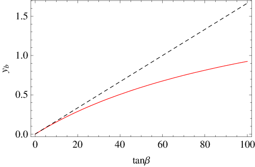
In the following, we will use this relation (11) to constrain lepton flavour violating parameters.

3 Constraints on the flavour-violating parameters

Various processes can be used to constrain lepton flavour violating (LFV) parameters. Remarkably, we can also use lepton flavor conserving (LFC) observables, due to double lepton flavour violation (LFV). Two LFV vertices lead to lepton flavor conservation (LFC) and so contribute to the LFC self-energies. In a similar manner, we will consider multiple flavour changes contributing to the magnetic moment of the electron. In addition, we consider LFV processes, in particular radiative decays.

As mentioned in the Introduction, we introduce the dimensionless parameters $\delta_{XY}^{ij}$ via

\displaystyle\Delta m_{XY}^{ij}=\delta_{XY}^{ij}\left(\overline{m}_{XY}^{ij}\right)^{2}=\delta_{XY}^{ij}\sqrt{m_{i_{X}}^{2}m_{j_{Y}}^{2}}\ ,\quad X,\,Y=R,\,L\ ,\quad i\not=j\ .

(16)

Note that $\Delta m_{XY}^{ij}$ has mass-dimension two. Both $m_{i_{X}}^{2}$ and $\Delta m_{XY}^{ij}$ are the diagonal and off-diagonal entries of the slepton mass matrix (87), so $\overline{m}_{XY}^{ij}$ is an average slepton mass.

The effects discussed in this section stem from chirally enhanced self-energies, which involve an extra factor of $\tan\beta$ compared to the tree-level result, analogous to $\epsilon_{b}$ in Eq. (15). Such effects have been widely studied before in the quark sector, yet most authors have performed their studies in the decoupling limit $M_{\rm SUSY}\gg v$ , where $M_{\rm SUSY}$ denotes the mass scale of the soft SUSY breaking parameters. (For a guide through the literature see Ref. [18].) If one relaxes the condition $M_{\rm SUSY}\gg v$ , novel effects (namely those which vanish like some power of $v/M_{\rm SUSY}$ ) can be analysed. Analytical results covering the case $M_{\rm SUSY}\sim v$ have been derived in Refs. [16, 19, 18, 20], numerical approaches were pursued in Refs. [21, 22]. Superparticle contributions to physical processes vanish for $M_{\rm SUSY}\to\infty$ , typically as $v^{2}/M_{\rm SUSY}^{2}$ , and can only be addressed with the methods of the latter papers. However, by combining the decoupling supersymmetric loop with resummation formulae valid for $M_{\rm SUSY}\gg v$ one can correctly reproduce the resummed all-order result to leading non-vanishing order in $v/M_{\rm SUSY}$ . This approach has been used in an analysis of “flavoured” electric dipole moments in Ref. [23].

The possibility to constrain $\delta_{XY}^{ij}$ through LFC processes has been pointed out in Ref. [24], which addresses leptonic Kaon decays. Here we analyse the constraints from two LFC observables which have not been considered before: In Sec. 3.1 we apply a naturalness argument to the electron mass, demanding that the supersymmetric loop corrections are smaller than the measured value. In Sec. 3.5 we study the anomalous magnetic moment of the electron.

3.1 Flavour-conserving self-energies

The masses of the SM fermions are protected from radiative corrections by the chiral symmetry $\Psi\rightarrow e^{i\alpha\gamma_{5}}\Psi$ . According to Weinberg, Susskind and ’t Hooft, a theory with small parameters is natural if the symmetry is enhanced when these parameters vanish. The smallness of the parameters is then protected against large radiative corrections by the concerned symmetry. This naturalness principle makes the smallness of the electron mass natural. Radiative corrections are proportional to the electron mass itself $\delta m_{e}\propto m_{e}\ln\left(\Lambda/m_{e}\right)$ and vanish for $m_{e}=0$ . If such a small parameter is composed of some different terms and one does not want any form of fine-tuning, one should require that all contributions should be roughly of the same order of magnitude; no accidental cancellation between different terms should occur. Hence, the counterterm of the electron mass should be less than the measured electron mass,

\displaystyle\left|\frac{\delta m_{e}}{m_{e}^{\text{phys}}}\right|=\left|\frac{m_{e}^{(0)}-m_{e}^{\text{phys}}}{m_{e}^{\text{phys}}}\right|<1\ .

(17)

This naturalness argument for the light fermion masses was already discussed in the pioneering study of Ref. [10]. Since the authors of this analysis want to provide a model-independent analysis on classes of SUSY theories they consider only photinos and do not include flavour violation in the corrections to light fermion masses. Their derived upper bound for $\delta_{LR}^{11}$ depends on the overall SUSY mass scale and actually becomes stronger for larger SUSY masses. The case of radiatively generated fermion masses via soft trilinear terms is studied in [25] and an updated version including two flavour-violating self-energies can be found in [26]. Here we concentrate on the chirality-conserving flavour-violating mass insertions and use this argument to restrict the product $\delta_{LL}^{13}\delta_{RR}^{13}$ which is then independent of the SUSY scale. Considering double lepton flavour violation, we demand that the radiative corrections should not exceed the tree-level contribution. For the electron mass, the dominant diagrams involve couplings to the third generation. As a result, we can constrain the product $\left|\delta_{LL}^{13}\delta_{RR}^{13}\right|$ . Note that $\left|\delta_{RR}^{13}\right|$ has so far been unconstrained from radiative decay $l_{j}\rightarrow l_{i}\gamma$ as we will discuss shortly in the following Section 3.2. This cancellation of the RR sensitivity is analysed in [11, 12] with the conclusion that even a better experimental sensitivity on $BR(l_{j}\to l_{i}\gamma)$ can not help to set strong constraints in the RR sector. However, with double mass insertions and the bound from $\mu\to e\gamma$ it is possible to derive bounds on products like $\delta_{LL}^{23}\delta_{RR}^{31}$ .

The diagram in Figure 3(a) achieves an $m_{\tau}\tan\beta$ enhancement only if there is a helicity flip in the stau propagator. Since $\alpha_{1}/\left(4\pi\right)\gg Y^{2}_{e}/\left(16\pi^{2}\right)$ , the higgsino contribution is negligible. A chargino loop can also be neglected, because only left-left (LL) insertions for the sneutrinos can be performed and the helicity flip is associated with an electron Yukawa coupling. The left-right (LR) insertions are either not associated with an $\tan\beta$ -enhanced contribution or suppressed by $v/M_{\text{SUSY}}$ , compared to right-right (RR) and LL-insertions. Thus the dominant diagram involves a Bino and the scalar tau-Higgs coupling, as shown in Figure 3(b).

Figure 3: (a) LFC self-energy through double LFV and (b) dominant double LFV contribution to the electron mass renormalisation.

For simplicity, we choose all parameters real and obtain

	$\displaystyle\Sigma_{e}^{\text{FV}}$	$\displaystyle\simeq\frac{\alpha_{1}}{4\pi}M_{1}\,\mu\,\frac{m_{\tau}^{\text{phys}}\tan\beta}{1+\Delta_{\tau}}\Delta m_{LL}^{13}\Delta m_{RR}^{13}\,F_{0}\left(M_{1}^{2},\,m_{\tilde{e}_{L}}^{2},\,m_{\tilde{e}_{R}}^{2},\,m_{\tilde{\tau}_{L}}^{2},\,m_{\tilde{\tau}_{R}}^{2}\right)$
		$\displaystyle\simeq-\frac{\alpha_{1}}{4\pi}M_{1}\,\mu\,\frac{m_{\tau}^{\text{phys}}\tan\beta}{1+\Delta_{\tau}}\Delta m_{LL}^{13}\Delta m_{RR}^{13}\,f_{1}^{\prime\prime}\left(M_{1}^{2},\,m_{\tilde{L}}^{2},\,m_{\tilde{R}}^{2}\right).$		(18)

For equal SUSY masses this simplifies to $\Sigma_{e}^{\text{FV}}=-\frac{\alpha_{1}}{48\pi}\frac{m_{\tau}\tan\beta}{1+\Delta_{\tau}}\delta_{LL}^{13}\delta_{RR}^{13}$ . This term is proportional to $m_{\tau}$ , in contrast to the LFC self energy, which is proportional to $m_{e}$ . Thus the counterterm receives an additional constant term $\Sigma_{e}^{\text{FV}}$ ,

Substituting $m^{\text{phys}}_{l}\to m^{\text{phys}}_{l}+\delta m^{(1)}_{l}$ , one gets the second order contributions since the only real diagrams of order $n$ are one-loop diagrams in which a counterterm of order $n-1$ is inserted.

We will use the on-shell renormalisation scheme, where the mass and the wave-function counterterms cancel all loop contributions to the self-energy such that the pole of the lepton propagator is equal to the physical mass of the lepton. Then we obtain the relation

\displaystyle m^{(0)}_{l}

\displaystyle=m^{\text{phys}}_{l}+\sum_{n=1}^{\infty}\delta m^{(n)}_{l}=\frac{m^{\text{phys}}_{l}}{1+\Delta_{l}}+\frac{\Sigma^{\text{FV}}_{l}}{1+\Delta_{l}}\ .

(19)

SPS	1a	1b	2	3	4	A	B
$m_{0}$	$100$	$200$	$1450$	$90$	$400$	$500$	$500$
$A_{0}$	$-100$	$0$	$0$	$0$	$0$	$0$	$0$
$m_{1/2}$	$250$	$400$	$300$	$400$	$300$	$500$	$500$
$\tan\beta$	$10$	$30$	$10$	$10$	$50$	$40$	$10$
$sgn(\mu)$	$+1$	$+1$	$+1$	$+1$	$+1$	$+1$	$+1$
$\mu(M_{Z})$	$352$	$507$	$422$	$516$	$388$	$614$	$629$

Table 1: Snowmass Points and Slopes [27] and two additional scenarios (masses in GeV)

For the numerical analysis, let us consider the mSUGRA scenario SPS4; its parameter values are given in Table 1. For this model, the constraint reads (Figure 4)

\displaystyle\left|\delta_{RR}^{13}\delta_{LL}^{13}\right|

\displaystyle<\begin{cases}0.097,&\text{if}\ \delta_{RR}^{13}\delta_{LL}^{13}>0\\[2.0pt] 0.083,&\text{if}\ \delta_{RR}^{13}\delta_{LL}^{13}<0\end{cases}

(20)

As discussed above, the constraint is independent of the overall SUSY mass scale. It does, however, depend on the ratio of the various masses, in particular $x=\mu/m_{R}$ . $m_{R,L}$ denotes the average right and left-handed slepton mass matrix, respectively. To be sure that this result is no special feature of SPS4, we consider other scenarios in Table 2, which differ by ratios of the SUSY breaking masses. The sparticle mass spectrum at the electroweak scale for SPS4 corresponds most likely to scenario 2 with $x\approx 0.9-1$ . The bounds are very strong for larger values of $x$ and weaken for a small $\mu$ -parameter. The upper bounds do not change considerably for values of $x$ larger than one and therefore are relatively stable and independent of the parameter space. Electroweak symmetry breaking yields a relation between the $\mu$ -Parameter, the mass of the $Z$ boson and the two Higgs fields such that in absence of any fine tuning $\mu^{2}$ should be within an order of magnitude of $M_{Z}^{2}$ (also known as the $\mu$ problem).

scenario		$x=0.3$	$x=1$	$x=1.5$	$x=3.0$	for
1	$M_{1}=M_{2}=m_{L}=m_{R}$	0.261	0.073	0.050	0.026	$\delta_{RR}^{13}\delta_{LL}^{13}>0$
1	$M_{1}=M_{2}=m_{L}=m_{R}$	0.234	0.059	0.040	0.023	$\delta_{RR}^{13}\delta_{LL}^{13}<0$
2	$3M_{1}=M_{2}=m_{L}=m_{R}$	0.301	0.083	0.057	0.029	$\delta_{RR}^{13}\delta_{LL}^{13}>0$
2	$3M_{1}=M_{2}=m_{L}=m_{R}$	0.269	0.067	0.045	0.024	$\delta_{RR}^{13}\delta_{LL}^{13}<0$
3	$M_{1}=M_{2}=3m_{L}=m_{R}$	0.292	0.082	0.057	0.031	$\delta_{RR}^{13}\delta_{LL}^{13}>0$
3	$M_{1}=M_{2}=3m_{L}=m_{R}$	0.235	0.067	0.042	0.027	$\delta_{RR}^{13}\delta_{LL}^{13}<0$
4	$M_{1}=M_{2}=\frac{m_{L}}{3}=m_{R}$	0.734	0.210	0.142	0.071	$\delta_{RR}^{13}\delta_{LL}^{13}>0$
4	$M_{1}=M_{2}=\frac{m_{L}}{3}=m_{R}$	0.702	0.190	0.127	0.064	$\delta_{RR}^{13}\delta_{LL}^{13}<0$
5	$3M_{1}=M_{2}=m_{L}=3m_{R}$	0.731	0.205	0.137	0.067	$\delta_{RR}^{13}\delta_{LL}^{13}>0$
5	$3M_{1}=M_{2}=m_{L}=3m_{R}$	0.693	0.179	0.116	0.054	$\delta_{RR}^{13}\delta_{LL}^{13}<0$

Table 2: Different mass scenarios and the corresponding upper bounds for

\left|\delta_{RR}^{13}\delta_{LL}^{13}\right|

m_{R,L}

denotes the average right and left-handed slepton mass, respectively,

M_{1}

and

M_{2}

the bino and wino masses. In all scenarios,

\tan\beta=50

and

\sgn(\mu)=+1

. The upper line is valid for

\delta_{RR}^{13}\delta_{LL}^{13}>0

, the lower for

\delta_{RR}^{13}\delta_{LL}^{13}<0

We will see in the following section that the dominating RR terms in the flavor violating self-energy $\tau\rightarrow e$ cancel in part of the parameter space. That is why so far no upper bound on $\delta_{RR}$ could be derived [11, 12]. In these regions, we can use the constraint on $\left|\delta_{RR}^{13}\delta_{LL}^{13}\right|$ as a restriction on $\delta_{RR}^{13}$ .

3.2 Lepton-flavour violating self-energies

Lepton flavour violating self-energies can be $\tan\beta$ -enhanced and, moreover, they also have a non-decoupling behaviour. They occur in the renormalisation of the PMNS matrix and lead to a correction of the radiative decays $l_{j}\rightarrow l_{i}\gamma$ .

We consider all diagrams with one LFV MI in the slepton propagator and start with $\tau_{R}\to e_{L}$ ; the dominant diagrams are shown in Figure 5. In fact, we can do an approximate diagonalisation of the neutralino mass matrix (83) and use the MI approximation in the slepton propagator. Furthermore, we will choose $\mu$ to be real.

The dominant diagrams are proportional to the mass of the tau and sensitive to the LL element (see diagram 1 to 3 in Fig. (5)), while the RR dependence is suppressed,

	$\displaystyle\Sigma_{\tau_{R}-e_{L}}^{\tilde{\chi}^{0}}$	$\displaystyle\simeq\frac{m_{\tau}^{\text{phys}}}{1+\Delta_{\tau}}\,\mu\,\tan\beta\;m_{\tilde{e}_{L}}m_{\tilde{\tau}_{L}}\delta_{LL}^{31}\left\{-\frac{\alpha_{1}}{4\pi}M_{1}\,f_{2}\left(M_{1}^{2},\,m_{\tilde{e}_{L}}^{2},\,m_{\tilde{\tau}_{R}}^{2},\,m_{\tilde{\tau}_{L}}^{2}\right)\right.$
		$\displaystyle\mspace{200mu}+\left.\left(-\frac{1}{2}\frac{\alpha_{1}}{4\pi}M_{1}\,+\frac{1}{2}\frac{\alpha_{2}}{4\pi}M_{2}\right)f_{2}\left(M_{1}^{2},\,\mu^{2},\,m_{\tilde{\tau}_{L}}^{2},\,m_{\tilde{e}_{L}}^{2}\right)\right\}.$		(21)

This self-energy will contribute to the renormalisation of the PMNS matrix (Section 3.3). As in the previous section, this contribution potentially leads to an upper bound on $\delta_{LL}^{13}$ when a naturalness argument is applied to the PMNS element $U_{e3}$ . Note that in Eq. (21) the LFC mass renormalisation is already taken into account.

Figure 5: Dominant diagrams for the neutralino-slepton and chargino-sneutrino loop for the

\tau_{R}\rightarrow e_{L}

-transition.

The dominant contributions for the opposite helicity transition, $\tau_{L}\to e_{R}$ , are analogous to the first and second diagrams in Fig. 5,

\displaystyle\Sigma_{\tau_{L}-e_{R}}^{\tilde{\chi}^{0}}

\displaystyle\simeq\frac{\alpha_{1}}{4\pi}\,\frac{m_{\tau}^{\text{phys}}}{1+\Delta_{\tau}}\,M_{1}\,\mu\,\tan\beta\;m_{\tilde{e}_{R}}m_{\tilde{\tau}_{R}}\delta_{RR}^{31}\left(f_{2}\left(M_{1}^{2},\,\mu^{2},\,m_{\tilde{\tau}_{R}}^{2},\,m_{\tilde{e}_{R}}^{2}\right)-f_{2}\left(M_{1}^{2},\,m_{\tilde{e}_{R}}^{2},\,m_{\tilde{\tau}_{R}}^{2},\,m_{\tilde{\tau}_{L}}^{2}\right)\right).

(22)

They are sensitive to the RR element; however, the relative minus sign due to the different hypercharges potentially leads to cancellations. In this approximation, the RR sensitivity vanishes completely for $\mu=m_{\tilde{\tau}_{L}}$ and hence no upper bounds on $\delta_{RR}^{ij}$ has been derived, as mentioned in the previous section. In Ref. [12] the processes $\mu\to e\gamma$ and $\mu\to e$ conversion in nuclei are combined. The corresponding one-loop amplitudes suffer from similar cancellations, albeit in different regions of the parameter space leading to the constraint $\delta_{RR}^{12}\leq 0.2$ .

Let us now turn to the chargino-sneutrino loops. As the left-handed charged sleptons and sneutrinos form a doublet, they have the same SUSY breaking soft mass and therefore the same off-diagonal elements. The neutrino is always left-handed so that the chargino loop can only be sensitive to the LL element and a chirality flip of the charged lepton is needed. The higgsino component of the chargino couples to the right-handed lepton and the wino part to the left-handed lepton. Thus, the self-energy is proportional to the mass of the right-handed lepton,

	$\displaystyle\Sigma_{l_{iL}-l_{jR}}^{\tilde{\chi}^{\pm}}$	$\displaystyle=\frac{g_{2}}{16\pi^{2}}Y_{j}\sum_{n=1}^{3}\sum_{k=1,2}Z_{-}^{2k}Z_{+}^{1k}Z_{\nu}^{jn}Z_{\nu}^{in*}m_{\tilde{\chi}_{k}}B_{0}\left(m_{\tilde{\nu}_{n}}^{2},m_{\tilde{\chi}_{k}^{\pm}}^{2}\right)$
		$\displaystyle\simeq\frac{\alpha_{2}}{4\pi}\,\frac{m_{j}^{\text{phys}}}{1+\Delta_{l_{j}}}\,M_{2}\,\mu\,\tan\beta\;m_{\tilde{\nu}_{i}}m_{\tilde{\nu}_{j}}\,\delta_{LL}^{ij}\,f_{2}\left(m_{\tilde{\nu}_{i}}^{2},m_{\tilde{\nu}_{j}}^{2},M_{2}^{2},\mu^{2}\right)\ .$		(23)

In the second line, we used the MI approximation in the chargino propagator and for the LFV (see last diagram in Fig. (5)).

3.3 PMNS matrix renormalisation

Up to now, we have only an upper bound for the matrix element $U_{e3}$ and thus for the mixing angle $\theta_{13}$ ; the best-fit value is at or close to zero (cf. Eq. (7)). It might well be that it vanishes at tree level due to a particular symmetry and obtains a non-zero value due to corrections. So we can ask the question if threshold corrections to the PMNS matrix could spoil the prediction $\theta_{13}=0^{\circ}$ at the weak scale. What does it mean for the physics at the high scale if experiment will tell us that $\theta_{13}$ does not vanish? As before, we demand the absence of fine-tuning for these corrections and therefore require that the SUSY loop contributions do not exceed the value of $U_{e3}$ ,

\displaystyle\left|\delta U_{e3}\right|\leq\left|U_{e3}^{\text{phys}}\right|.

(24)

Then we can in principle use the smallness of $U_{e3}$ to constrain $\delta_{LL}^{13}$ .

In an effective field theory approach, the renormalisation of the PMNS matrix is done via rotation matrices that diagonalise the mass matrix, which receives contribution from both the tree-level coupling of the fermions to $H_{d}$ and the loop-induced coupling to $H_{u}$ (see Refs. [13, 28, 29, 21] for the quark sector). Lepton flavour violating self-energies induce off-diagonal entries in the mass matrix. In order to deal with physical fields, one has to rotate them in flavour space to achieve a diagonal mass matrix.

As a drawback, the effective field theory method is only valid if the masses of the supersymmetric particles in the loop are much larger than $v=174$ GeV. For sleptons and neutralinos this assumption is doubtful, so that we resort to the diagrammatic method of Refs. [16, 17, 18] which does not rely on any hierarchy between $M_{\rm SUSY}$ and $v$ . In our diagrammatic approach, we consider chargino and neutralino loops in the external lepton propagator and resum all $\tan\beta$ -enhanced corrections explicitly. Once again the on-shell scheme is used. The loop corrections are finite and the counterterms are defined such that they exactly cancel the loop diagrams:

\displaystyle U^{(0)}=U^{\text{phys}}+\sum_{n}\delta U^{(n)}=U^{\text{phys}}+\delta U\ .

(25)

The first-order correction is displayed in the adjoining figure. The counterterm reads

	$\displaystyle\delta U_{jk}^{(1)}$	$\displaystyle=\sum_{l\neq j}U_{lk}^{\text{phys}}\frac{(\not{p}_{j}+m_{l})}{p_{j}^{2}-m_{l}^{2}}\left(\Sigma_{l_{j}-l_{l}}\right)^{*}$
		$\displaystyle\simeq\begin{cases}\sum_{l\neq j}U_{lk}^{\text{phys}}\frac{1}{m_{j}}\left(\Sigma_{l_{jR}-l_{lL}}\right)^{},&j>l\ ,\ \textrm{i.e., heavy particle as external leg;}\\ -\sum_{l\neq j}U_{lk}^{\text{phys}}\frac{1}{m_{l}}\left(\Sigma_{l_{jL}-l_{lR}}\right)^{},&j<l\ ,\ \textrm{i.e., heavy particle as internal propagator.}\end{cases}$		(26)

As for the mass renormalisation there are no genuine $\tan\beta$ -enhanced two-loop diagrams. The corrections in second order come from one-loop diagrams in which a counterterm of first order is inserted, corresponding to the substitution $U_{lk}^{\text{phys}}\to U_{lk}^{\text{phys}}+\delta U_{lk}^{(1)}$ . In contrast to the resummation of the mass counterterms, these counterterms are not directly proportional to the PMNS-element under consideration. The sum of the counterterms has to cancel the corrections up to that order, so at the $n^{\text{th}}$ order, one gets

\displaystyle\sum_{m=1}^{n}\delta U_{jk}^{(m)}

\displaystyle=\begin{cases}\sum_{l\neq j}\left(U_{lk}^{\text{phys}}+\sum_{m}^{n-1}\delta U_{lk}^{(m)}\right)\frac{1}{m_{j}}\left(\Sigma_{l_{jR}-l_{lL}}\right)^{*}\ ,&j>l\\ -\sum_{l\neq j}\left(U_{lk}^{\text{phys}}+\sum_{m}^{n-1}\delta U_{lk}^{(m)}\right)\frac{1}{m_{l}}\left(\Sigma_{l_{jL}-l_{lR}}\right)^{*}\ ,&j<l\end{cases}.

(27)

Now we can take the limit $n\to\infty$ and obtain a linear system of equations for the $U^{(0)}$ elements ( $k=1,\,2,\,3$ ):


$\displaystyle U_{ek}^{(0)}+\frac{1}{m_{\mu}}\Sigma_{\mu_{R}-e_{L}}U_{\mu k}^{(0)}+\frac{1}{m_{\tau}}\Sigma_{\tau_{R}-e_{L}}U_{\tau k}^{(0)}=$	$\displaystyle U_{ek}^{\text{phys}},$	(28a)
$\displaystyle U_{\mu k}^{(0)}-\frac{1}{m_{\mu}}\Sigma_{e_{L}-\mu_{R}}U_{ek}^{(0)}+\frac{1}{m_{\tau}}\Sigma_{\tau_{R}-\mu_{L}}U_{\tau k}^{(0)}=$	$\displaystyle U_{\mu k}^{\text{phys}},$	(28b)
$\displaystyle U_{\tau k}^{(0)}-\frac{1}{m_{\tau}}\Sigma_{e_{L}-\tau_{R}}U_{ek}^{(0)}-\frac{1}{m_{\tau}}\Sigma_{\mu_{L}-\tau_{R}}U_{\mu k}^{(0)}=$	$\displaystyle U_{\tau k}^{\text{phys}}.$	(28c)

In the MSSM, we have $\Sigma=\Sigma^{\tilde{\chi}^{0}}+\Sigma^{\tilde{\chi}^{\pm}}$ . As shown above, $\Sigma_{\tau_{R}-e_{L}}$ is sensitive to $\delta_{LL}^{13}$ and so is $\delta U_{e3}$ . We aim to avoid accidental cancellations and set all off-diagonal elements to zero except for $\delta_{LL}^{13}$ ²² 2 In [26] we study the case with nonvanishing $\delta_{LR}^{13}$ .. In this case we can explicitly solve the linear system of equations

\displaystyle U_{e3}^{(0)}=\frac{U_{e3}^{\text{phys}}-\frac{1}{m_{\tau}}\Sigma_{\tau_{R}-e_{L}}U_{\tau 3}^{\text{phys}}}{1+\left|\frac{1}{m_{\tau}}\Sigma_{\tau_{R}-e_{L}}\right|^{2}}.

(29)

By means of Eq. (24), we can in principle derive upper bounds for $\delta_{LL}^{13}$ . As shown in Figs. 6, they strongly depend on $\tan\beta$ and the assumed value for $U_{e3}^{\text{phys}}$ .

After three years of running, the DOUBLE CHOOZ experiment will be sensitive to $\theta_{13}=3^{\circ}$ , which corresponds to $U_{e3}=0.05$ . A future neutrino factory may probe $\theta_{13}$ down to $\theta_{13}=0.6^{\circ}$ [30]. In general, even with future experimental facilities, we can conclude that the corrections from SUSY loops to the small element $U_{e3}$ stay unobservably small. This means at the same time that if some experiment measures $\theta_{13}\neq 0$ , this will not be compatible with tri-bimaximal mixing at the high scale and moderate sparticle masses, since SUSY threshold corrections cannot account for such an effect: Even for large $\tan\beta$ the already existing constraints on $\delta_{LL}^{13}$ from $\tau\rightarrow e\gamma$ are stronger assuming reasonable SUSY masses. However, since $\tau\rightarrow e\gamma$ decouples, our method leads to a sharper bound for very large SUSY masses, especially with $\theta_{13}=1^{\circ}$ and large $\tan\beta$ .

3.4 Counterterms in the flavour basis and charged Higgs couplings

Neutrinos are both produced and detected as flavour eigenstates. In order to have flavour diagonal $W$ couplings, however, it is necessary to introduce counterterms, $\delta V_{ij}$ , which cancel the LFV loops. By doing this you perform a renormalisation of the unit matrix. In an effective field theory approach this is achieved via a wave function renormalisation by rotating the lepton fields leading to a diagonal mass matrix and physical fields. This rotation of the fields induce LFV in the charged Higgs coupling to lepton and neutrino and the same is true for the counterterms in the diagrammatic approach.

The first-order correction is displayed in the figure above; the flavour-diagonal vertices do not get any counterterms, since the external loops are already included in the mass renormalisation. We obtain

\displaystyle\delta V

\displaystyle=\begin{pmatrix}0&-\frac{1}{m_{\mu}^{\text{phys}}}\Sigma_{e_{L}-\mu_{R}}&-\frac{1}{m_{\tau}^{\text{phys}}}\Sigma_{e_{L}-\tau_{R}}\\[2.0pt] \frac{1}{m_{\mu}^{\text{phys}}}\Sigma_{\mu_{R}-e_{L}}&0&-\frac{1}{m_{\tau}^{\text{phys}}}\Sigma_{\mu_{L}-\tau_{R}}\\[2.0pt] \frac{1}{m_{\tau}^{\text{phys}}}\Sigma_{\tau_{R}-e_{L}}&\frac{1}{m_{\tau}^{\text{phys}}}\Sigma_{\tau_{R}-\mu_{R}}&0\end{pmatrix}.

(30)

You can translate this to the mass eigenstate basis used in Eq. (28) via $\delta U_{ik}=\delta V_{ij}^{*}U_{jk}^{(0)}$ . These counterterms induce LFV in the charged Higgs coupling to lepton and neutrino, due to the different helicity structure of the Higgs and $W$ coupling and the different lepton masses. The $H^{+}e\nu_{\tau}$ vertex can be of particular importance, since it is possible to pick up terms with a tau Yukawa coupling. As discussed before, this coupling is enhanced in the large $\tan\beta$ regime and can partly compensate the loop suppression factor.

The chargino contributions from the counterterm and the LFV loop cancel in the charged Higgs coupling as the chargino loop is exactly proportional to the mass of the right handed lepton. Therefore only the neutralino contributions remain.

The charged Higgs coupling to electrons reads


$\displaystyle i\Gamma^{H^{+}}_{e\nu_{\tau}}$	$\displaystyle=\frac{ig_{2}}{\sqrt{2}M_{W}}\tan\beta\left(m_{e}^{(0)}\,\delta V_{13}+m_{\tau}^{(0)}\frac{\Sigma_{e_{R}-\tau_{L}}}{m_{\tau}^{\text{phys}}}\right)=\frac{ig_{2}}{\sqrt{2}M_{W}}\tan\beta\left(-\frac{m_{e}^{\text{phys}}}{m_{\tau}^{\text{phys}}}\frac{\Sigma_{e_{L}-\tau_{R}}}{1+\Delta_{e}}+\frac{\Sigma_{e_{R}-\tau_{L}}}{1+\Delta_{\tau}}\right),$	(31a)
$\displaystyle i\Gamma^{H^{+}}_{e\nu_{\mu}}$	$\displaystyle=\frac{ig_{2}}{\sqrt{2}M_{W}}\tan\beta\left(m_{e}^{(0)}\delta V_{12}+m_{\mu}^{(0)}\frac{\Sigma_{e_{R}-\mu_{L}}}{m_{\mu}^{\text{phys}}}\right)=\frac{ig_{2}}{\sqrt{2}M_{W}}\tan\beta\left(-\frac{m_{e}^{\text{phys}}}{m_{\mu}^{\text{phys}}}\frac{\Sigma_{e_{L}-\mu_{R}}}{1+\Delta_{e}}+\frac{\Sigma_{e_{R}-\mu_{L}}}{1+\Delta_{\mu}}\right),$	(31b)
$\displaystyle i\Gamma^{H^{+}}_{e\nu_{e}}$	$\displaystyle=\frac{ig_{2}}{\sqrt{2}M_{W}}\frac{m_{e}^{\text{phys}}}{1+\Delta_{e}}\tan\beta\left(1+\frac{m_{\tau}^{\text{phys}}}{m_{e}^{\text{phys}}}\frac{\tan\beta}{1+\Delta_{\tau}}\Delta^{e}_{LR}\right),$	(31c)

where $\Sigma^{\text{FV}}_{e}=\frac{m_{\tau}^{\text{phys}}}{1+\Delta_{\tau}}\,\tan\beta\;\Delta_{LR}^{e}$ . We see that the counterterms are suppressed with the electron mass. As the lepton mass cancels out in $\Sigma_{e_{R}-\ell_{iL}}/m_{\ell_{i}}$ , the LFV loop contributions with $\nu_{\tau}$ and $\nu_{\mu}$ differ by a factor $m_{\tau}/m_{\mu}$ .

Similarly, we obtain for the coupling to muons,


$\displaystyle i\Gamma^{H^{+}}_{\mu\nu_{\tau}}$	$\displaystyle=\frac{ig_{2}}{\sqrt{2}M_{W}}\tan\beta\left(m_{\mu}^{(0)}\delta V_{23}+m_{\tau}^{(0)}\frac{\Sigma_{\mu_{R}-\tau_{L}}}{m_{\tau}^{\text{phys}}}\right)=\frac{ig_{2}}{\sqrt{2}M_{W}}\tan\beta\left(-\frac{m_{\mu}^{\text{phys}}}{m_{\tau}^{\text{phys}}}\frac{\Sigma_{\mu_{L}-\tau_{R}}}{1+\Delta_{\mu}}+\frac{\Sigma_{\mu_{R}-\tau_{L}}}{1+\Delta_{\tau}}\right),$	(32a)
$\displaystyle i\Gamma^{H^{+}}_{\mu\nu_{\mu}}$	$\displaystyle=\frac{ig_{2}}{\sqrt{2}M_{W}}\frac{m_{\mu}^{\text{phys}}}{1+\Delta_{\mu}}\tan\beta\left(1+\frac{m_{\tau}^{\text{phys}}}{m_{\mu}^{\text{phys}}}\frac{\tan\beta}{1+\Delta_{\tau}}\Delta^{\mu}_{LR}\right).$	(32b)
$\displaystyle i\Gamma^{H^{+}}_{\mu\nu_{e}}$	$\displaystyle=\frac{ig_{2}}{\sqrt{2}M_{W}}\tan\beta\left(m_{\mu}^{(0)}\delta V_{21}-m_{e}^{(0)}\frac{\Sigma_{\mu_{R}-e_{L}}}{m_{e}^{\text{phys}}}\right)=\frac{ig_{2}}{\sqrt{2}M_{W}}\tan\beta\left(\frac{\Sigma_{\mu_{L}-e_{R}}}{1+\Delta_{\mu}}-\frac{m_{e}^{\text{phys}}}{m_{\mu}^{\text{phys}}}\frac{\Sigma_{\mu_{R}-e_{L}}}{1+\Delta_{e}}\right),$	(32c)

While the first term is similar to the couplings to electrons, the counterterm dominates over the loop contribution if there is an electron neutrino in the final state.

Finally, for the $\tau$ coupling one finds


$\displaystyle i\Gamma^{H^{+}}_{\tau\nu_{\tau}}$	$\displaystyle=\frac{ig_{2}}{\sqrt{2}M_{W}}\frac{m_{\tau}^{\text{phys}}}{1+\Delta_{\tau}}\tan\beta\ ,$	(33a)
$\displaystyle i\Gamma^{H^{+}}_{\tau\nu_{\mu}}$	$\displaystyle=\frac{ig_{2}}{\sqrt{2}M_{W}}\tan\beta\left(m_{\tau}^{(0)}\delta V_{32}-m_{\mu}^{(0)}\frac{\Sigma_{\tau_{L}-\mu_{R}}}{m_{\tau}^{\text{phys}}}\right)=\frac{ig_{2}}{\sqrt{2}M_{W}}\tan\beta\left(\frac{\Sigma_{\tau_{R}-\mu_{L}}}{1+\Delta_{\tau}}-\frac{m_{\mu}^{\text{phys}}}{m_{\tau}^{\text{phys}}}\frac{\Sigma_{\tau_{L}-\mu_{R}}}{1+\Delta_{\mu}}\right),$	(33b)
$\displaystyle i\Gamma^{H^{+}}_{\tau\nu_{e}}$	$\displaystyle=\frac{ig_{2}}{\sqrt{2}M_{W}}\tan\beta\left(m_{\tau}^{(0)}\delta V_{31}-m_{e}^{(0)}\frac{\Sigma_{\tau_{L}-e_{R}}}{m_{\tau}^{\text{phys}}}\right)=\frac{ig_{2}}{\sqrt{2}M_{W}}\tan\beta\left(\frac{\Sigma_{\tau_{R}-e_{L}}}{1+\Delta_{\tau}}-\frac{m_{e}^{\text{phys}}}{m_{\tau}^{\text{phys}}}\frac{\Sigma_{\tau_{L}-e_{R}}}{1+\Delta_{e}}\right).$	(33c)

The results of Eqs. (31)-(33) are given in Eqs. (92-95) of Ref. [23] for the decoupling limit $M_{\rm SUSY}\gg v$ . In Appendix C of Ref. [23] an iterative procedure (analogous to the one in Ref. [21]) has been outlined which achieves the all-order resummation of the $\tan\beta$ -enhanced higher-order corrections. Eqs. (31)-(33) comprise analytical formulae for the limits to which this iterative procedure converges.

The $\tan\beta$ -enhanced lepton flavour violating Higgs couplings can become important in the leptonic decay of charged Kaons, $K\rightarrow l\nu$ , where they potentially induce lepton non-universality. Then the current experimental data and our fine-tuning argument together constrain the various terms in Eqs. (31), as they contribute to the electron self-energy as well. In particular, if the second term in Eq. (31c) had a significant effect in the ratio $R_{K}=\Gamma(K\rightarrow e\nu)/\Gamma(K\rightarrow\mu\nu)$ , as was assumed in Ref. [24], $\Delta^{e}_{LR}$ would give a large contribution to the electron mass [31]. (The value $\Delta_{RL}^{11}\stackrel{{\scriptstyle\scriptscriptstyle\wedge}}{{=}}\Delta_{LR}^{e}=10^{-4}$ [24] corresponds to $\delta_{RR}^{13}\delta_{LL}^{13}\approx 2$ in the SPS4 scenario and thus gives a more than 2000% correction to the electron mass.) While in the improved analysis [32] the contribution of $\Sigma_{e}^{FV}$ to the electron mass was not considered, their scanned values of $\delta_{LL,RR}^{13}$ are in agreement with the fine-tuning argument. The scan respects $\left|\delta_{LL}^{13}\delta_{RR}^{13}\right|\leq 0.25$ , in marginal agreement with our results of Sects. 3.1 and 3.5. The NA62 experiment at CERN aims to reduce the error of $R_{K}$ from $1.3\%$ to $0.3\%$ . This prospective error is used in Ref. [33] to derive large, phenomenologically interesting values for $\delta_{LL}^{13}$ and $\delta_{RR}^{13}$ .

3.5 Anomalous Magnetic Moment of the Electron

The anomalous magnetic moment of the electron plays a central role in quantum electrodynamics. The precise measurements provide the best source of the fine structure constant $\alpha_{\text{em}}$ if one assumes the validity of QED [34]. Conversely, one can use a value of $\alpha_{\text{em}}$ from a (less precise) measurement and insert it into the theory prediction for $a_{e}$ to probe new physics in the latter quantity. The most recent calculation yields [35]

\displaystyle a_{e}

\displaystyle=1\;159\;652\;182.79\left(7.71\right)\times 10^{-12}\;,

(34)

where the largest uncertainty comes from the second-best measurement of $\alpha_{\text{em}}$ which is $\alpha_{\text{em}}^{-1}=137.03599884(91)$ from a Rubidium atom experiment [36].

Supersymmetric contributions to the magnetic moment are usually small, due to the smallness of the electron Yukawa coupling and the SUSY mass suppression. However, multiple flavour changes, resulting in a LFC loop, insert the $\tau$ Yukawa coupling, which strongly enhances the amplitude. As a result, supersymmetric contributions can be as large as $\mathcal{O}(10^{-12})$ , comparable to the weak or hadronic contributions [35]. The amplitude can exceed a $3\sigma$ deviation of the theoretical mean value, which enables us to constrain the LFV parameters $\delta^{13}_{LL}$ and $\delta^{13}_{RR}$ . In Ref. [11] the magnetic and electric dipole moments $a_{i}$ and $d_{i}$ of the charged lepton $\ell_{i}$ were calculated in the MSSM, considering flavour-conserving and flavour-violating contributions within the mass insertion approximation. The authors found that the naïve mass scaling can be overcome with double mass insertions. However, in their phenomenological analysis to constrain the flavour-violating parameters $\delta_{XY}^{ij}$ , they only used $a_{\mu}$ and the experimental bounds on $d_{\mu}$ and $d_{e}$ but did not consider $a_{e}$ . Our consideration of $a_{e}$ adds a novel aspect to the phenomenological study of LFV parameters in the MSSM and complements the analysis of Ref. [11] in this respect.

The supersymmetric contributions to the anomalous magnetic moment $a_{e}$ are generated by chargino and neutralino loops, where the photon couples to any charged particle in the loop. The full analytic result can be found in Ref. [37]. Here, we will neglect the terms which are both proportional to the electron mass and not (potentially) $\tan\beta$ -enhanced and are therefore left with


$\displaystyle a^{\chi^{0}}_{e}$	$\displaystyle=-\frac{m_{e}}{16\pi^{2}}\sum_{A=1}^{4}\sum_{X=1}^{6}\frac{m_{\chi^{0}_{A}}}{3m^{2}_{\tilde{l}_{X}}}\re\left[N^{L}_{1AX}N^{R\ast}_{1AX}\right]F_{2}^{N}\left(x_{AX}\right),$	$\displaystyle x_{AX}$	$\displaystyle=\frac{m_{\tilde{\chi}^{0}_{A}}^{2}}{m_{\tilde{l}_{X}}^{2}},$	(35a)
$\displaystyle a^{\chi^{\pm}}_{e}$	$\displaystyle=\frac{m_{e}}{16\pi^{2}}\sum_{A=1,2}\sum_{X=1}^{3}\frac{2m_{\chi^{\pm}_{A}}}{3m^{2}_{\tilde{\nu}_{X}}}\re\left[C^{L}_{1AX}C^{R\ast}_{1AX}\right]F_{2}^{C}\left(x_{AX}\right),$	$\displaystyle x_{AX}$	$\displaystyle=\frac{m_{\tilde{\chi}^{\pm}_{A}}^{2}}{m_{\tilde{\nu}_{X}}^{2}}.$	(35b)

The loop functions are listed in Eq. (80) and the couplings read [38]


$\displaystyle N_{iAX}^{L}$	$\displaystyle=-\sqrt{2}g_{1}\left(Z_{L}^{i+3,X}\right)^{}Z_{N}^{1A}+Y_{l_{i}}\left(Z_{L}^{i,X}\right)^{}Z_{N}^{3A}=\left(\Gamma_{l_{iR}}^{\tilde{\chi}^{0}_{A}\tilde{l}_{X}}\right)^{*},$	(36a)
$\displaystyle N_{iAX}^{R}$	$\displaystyle=\frac{(Z_{L}^{i,X})^{}}{\sqrt{2}}\left(g_{1}\left(Z_{N}^{1A}\right)^{}+g_{2}\left(Z_{N}^{2A}\right)^{}\right)+Y_{l_{i}}\left(Z_{N}^{3A}\right)^{}\left(Z_{L}^{i+3,X}\right)^{}=\left(\Gamma_{l_{iL}}^{\tilde{\chi}^{0}_{A}\tilde{l}_{X}}\right)^{},$	(36b)
$\displaystyle C_{iAX}^{L}$	$\displaystyle=-Y_{l_{i}}Z_{-}^{2A}Z_{\nu}^{i,X}=\left(\Gamma_{l_{iR}}^{\tilde{\chi}^{\pm}_{A}\tilde{\nu}_{X}}\right)^{*},$	(36c)
$\displaystyle C_{iAX}^{R}$	$\displaystyle=-g_{2}\left(Z_{+}^{1A}\right)^{}Z_{\nu}^{i,X}=\left(\Gamma_{l_{iL}}^{\tilde{\chi}^{\pm}_{A}\tilde{\nu}_{X}}\right)^{}.$	(36d)

The mixing matrices are defined in Appendix B. Note that they are $6\times 6$ matrices, in order to allow for flavour changes in the loop.

The dependence on $\tan\beta$ in Eqs. (35) is hidden in the mixing matrices. In principle, $\tan\beta$ comes from a chirality flip on the selectron line and in the chargino case from the combination of vacuum expectation value $v_{u}$ and the Yukawa coupling, $y_{e}v_{u}=m_{e}\tan\beta$ . We can, however, simplify the expressions significantly as follows: We assume a universal SUSY mass, real parameters and the same signs for $M_{1}$ and $M_{2}$ [39], then expand $a_{e}$ in powers of $M_{W}/M_{\text{SUSY}}$ or $1/\tan\beta$ . Then we obtain

\displaystyle\begin{split}a^{\chi^{0}}_{e}&=\sgn\left(\mu M_{2}\right)\frac{g^{2}_{1}-g^{2}_{2}}{192\pi^{2}}\frac{m^{2}_{e}}{M^{2}_{\text{SUSY}}}\tan\beta\left[1+\mathcal{O}\left(\frac{1}{\tan\beta},\,\frac{M_{W}}{M_{\text{SUSY}}}\right)\right],\\ a^{\chi^{\pm}}_{e}&=\sgn\left(\mu M_{2}\right)\frac{g^{2}_{2}}{32\pi^{2}}\frac{m^{2}_{e}}{M^{2}_{\text{SUSY}}}\tan\beta\left[1+\mathcal{O}\left(\frac{1}{\tan\beta},\,\frac{M_{W}}{M_{\text{SUSY}}}\right)\right].\end{split}

(37)

The result is again finite. The $1/M_{\text{SUSY}}^{2}$ dependence reflects the decoupling behaviour of supersymmetry. Furthermore, we note that a large value for $\tan\beta$ can dilute the $1/M_{\text{SUSY}}^{2}$ suppression. The numerical results are computed with the exact formula in Eqs. (35).

So far, the Yukawa couplings are unrenormalised; the inclusion of the mass renormalisation amounts to a loop contribution to $a_{e}$ which approximately grows as $\tan^{2}\beta$ [17]. Diagonalising the mixing matrices perturbatively, one finds a linear dependence on the Yukawa coupling of the remaining second terms of Eqs. (35). In this way we find an easy expression, which takes the corrections into account by a global factor,

\displaystyle a_{e}^{\text{SUSY},\,1L}+a_{e}^{\text{SUSY},\Delta_{e}}=a_{e}^{\text{SUSY},\,1L}\left(\frac{1}{1+\Delta_{e}}\right),

(38)

where $a_{e}^{\text{SUSY},\,1L}=a^{\chi^{0}}_{e}+a^{\chi^{\pm}}_{e}$ , as discussed in Ref. [17].

For the numerical analysis, we only allow $\delta^{13}_{LL}$ and $\delta^{13}_{RR}$ to be non-zero such that they are the only source of flavour violation. The theoretical uncertainty in Eq. (34) is taken as $1\sigma$ deviation and we require that the SUSY contribution to $a_{e}$ is less than $3\sigma$ .

We show the results for our scenarios 2 and 5 (see Table 2) in Fig. 7. As $\delta^{13}_{RR}$ increases, the bound on $\delta^{13}_{LL}$ becomes stronger and vice versa. The bound strongly depends on the SUSY mass. Since $a_{e}$ decouples for large SUSY masses, the bounds become very loose for $M_{\text{SUSY}}\gtrsim 500$ GeV. On the other hand, small SUSY masses lead to complex slepton masses, resulting in a lower bound on the SUSY mass. For this reason, the upper bounds on $\delta^{13}_{LL}$ and $\delta^{13}_{RR}$ are limited by the SUSY mass constraints. We find $\left|\delta^{13}_{LL}\cdot\delta^{13}_{RR}\right|<0.1$ for $M_{\text{SUSY}}\stackrel{{\scriptstyle<}}{{{}_{\sim}}}500$ GeV, coinciding with our non-decoupling bound in Eq. (20).

3.6 The radiative decay $l_{j}\rightarrow l_{i}\gamma$

Since their SM branching ratios are tiny, supersymmetric contributions to lepton flavour violating decays $l_{i}\rightarrow l_{j}\gamma$ can be sizable and vastly dominate over the SM values. As indicated above, these decays currently give the best constraints on the left-left (LL) and left-right (LR) lepton flavour violating parameters. At one-loop level and within MIA, $l_{i}\rightarrow l_{j}\gamma$ has for example extensively been studied in Ref. [11], constraining e.g. the mSUGRA parameters $M_{1}$ and $m_{R}$ . In this section, we compute the supersymmetric contributions to $l_{i}\rightarrow l_{j}\gamma$ , including both the mass renormalisation and the two-loop contributions coming from flavour-violating loops. The current upper bounds for the branching ratios are listed in Table 3.

experimental upper bounds
BR $\left(\mu\rightarrow e\gamma\right)$	$1.2\cdot 10^{-11}$
BR $\left(\tau\rightarrow e\gamma\right)$	$1.1\cdot 10^{-7}$
BR $\left(\tau\rightarrow\mu\gamma\right)$	$6.8\cdot 10^{-8}$

Table 3: Current upper bounds for BR

\left(l_{j}\rightarrow l_{i}\gamma\right)

j>i

[40].

Let us briefly summarise the formalism. Three SUSY diagrams contribute to the amplitude of $l_{j}\rightarrow l_{i}\gamma$ , corresponding to the coupling of the photon to $l_{j}$ , $l_{i}$ , and the charged particle in the loop. The off shell amplitude can be written as [41]

\displaystyle i\mathcal{M}=ie\epsilon^{\mu*}\overline{u}_{i}(p-q)\left[q^{2}\gamma_{\mu}(A_{1}^{L}P_{L}+A_{1}^{R}P_{R})+m_{l_{j}}i\sigma_{\mu\nu}q^{\nu}(A_{2}^{L}P_{L}+A_{2}^{R}P_{R})\right]u_{j}(p)\ ,

(39)

where $\epsilon^{*}$ is the photon polarisation vector. If the photon is on shell, the first part of the off-shell amplitude vanishes.

The coefficients $A$ contain chargino and neutralino contributions,

\displaystyle A^{L,R}=A^{(\tilde{\chi}^{0})L,R}+A^{(\tilde{\chi}^{\pm})L,R},\quad i=1,2\ ,

(40)

so $A^{L}$ is given by the sum of [42]

	$\displaystyle A_{2}^{(\tilde{\chi}^{0})L}$	$\displaystyle=\frac{1}{32\pi^{2}}\sum_{A=1}^{4}\sum_{X=1}^{6}\frac{1}{m_{\tilde{l}_{X}}^{2}}\left[N_{iAX}^{L}N_{jAX}^{L}\frac{1}{12}F_{1}^{N}(x_{AX})+N_{iAX}^{L}N_{jAX}^{R}\frac{m_{\tilde{\chi}^{0}_{A}}}{3m_{l_{j}}}F_{2}^{N}(x_{AX})\right],$		(41)
	$\displaystyle A_{2}^{(\tilde{\chi}^{\pm})L}$	$\displaystyle=-\frac{1}{32\pi^{2}}\sum_{A=1}^{2}\sum_{X=1}^{3}\frac{1}{m_{\tilde{\nu}_{X}}^{2}}\left[C_{iAX}^{L}C_{jAX}^{L}\frac{1}{12}F_{1}^{C}(x_{AX})+C_{iAX}^{L}C_{jAX}^{R}\frac{2m_{\tilde{\chi}^{\pm}_{A}}}{3m_{l_{j}}}F_{2}^{C}(x_{AX})\right],$		(42)

with the couplings given in Eqs. (36). We get $A^{R}$ by simply interchanging $L\leftrightarrow R$ .

Finally, the decay rate is given by

\displaystyle\Gamma(l_{j}\rightarrow l_{i}\gamma)=\frac{e^{2}}{16\pi}m^{5}_{l_{j}}\left(\left|A^{L}_{2}\right|^{2}+\left|A^{R}_{2}\right|^{2}\right).

(43)

Both the flavor-conserving transition $l_{i}\rightarrow l_{i}\gamma$ and the flavour-changing self-energies are $\tan\beta$ -enhanced. For this reason, we do not only consider the effect of the mass renormalisation but also include the two-loop contributions. Because of the double $\tan\beta$ enhancement they can compete with the first non-vanishing contribution. As for the corresponding counterterms, mass counterterms have to be inserted. In addition, wave-function renormalisation counterterms play a role as the above-quoted result for $l_{j}\rightarrow l_{i}\gamma$ presumes an expansion in the external momenta of the lepton. Therefore, to be consistent, the counterterm has to be given in higher order of the external momentum. However, only the mass counterterm will be $\tan\beta$ -enhanced because of the chirality flip involved. Corresponding diagrams are shown in Figs. 8.

The wave-function and mass counterterms are given by:

\displaystyle l_{L}^{0}

\displaystyle=\left(1+\frac{1}{2}\delta l_{L}\right)l_{L}\,,

\displaystyle l_{R}^{0}

\displaystyle=\left(1+\frac{1}{2}\delta l_{R}\right)l_{R}\,,

\displaystyle m_{l}^{0}

\displaystyle=m_{l}+\delta m_{l}\,,

(44)

where the fields and masses with a superscript 0 are the unrenormalised fields. In order to identify the counterterms, one first considers the kinetic and the mass term of the Lagrangian. The one-loop self-energy of the lepton can be divided into a scalar and a vector-type part, where the latter can further be divided in a left-left and a right-right transition,

\displaystyle i\Sigma_{l}(p)=i\Sigma_{l_{L}-l_{R}}^{S}(p)+i\not{p}\,\Sigma_{l_{L}-l_{L}}(p)P_{L}+i\not{p}\,\Sigma_{l_{R}-l_{R}}(p)P_{R}\ .

(45)

Now we demand that the additional terms in the mass Lagrangian cancel the scalar-part of the one-loop self-energy whereas the additional terms in the wave-function Lagrangian cancel the vector-type part. Therefore the counterterms have to fulfil the following conditions:

	$\displaystyle\delta l_{L}$	$\displaystyle=-\Sigma_{l_{L}-l_{L}}(p^{2}=m_{l}^{2}),$	$\displaystyle\quad\delta l_{R}$	$\displaystyle=-\Sigma_{l_{R}-l_{R}}(p^{2}=m_{l}^{2})\ ,$		(46)
	$\displaystyle\delta m_{l}$	$\displaystyle=\Sigma_{l_{L}-l_{R}}(p^{2}=m_{l}^{2})-\frac{m_{l}}{2}(\delta l_{L}+\delta l_{R})\ .\quad$				(47)

To give an explicit expression for the counterterms, we expand the self-energies up to the quadratic order in the external momentum and then compute the two parts of the one-loop self-energy. In the series, the even and odd orders contribute to the scalar and the vector type part, respectively. The chargino contribution to the counterterm is then given by

$\displaystyle\delta m_{l}$	$\displaystyle=\frac{1}{16\pi^{2}}\sum_{k}\Gamma_{l,\tilde{\nu},\tilde{\chi}_{k}}\Gamma^{*}_{l,\tilde{\nu},\tilde{\chi}_{k}}\left(-B_{0}+m^{2}_{l}m_{\tilde{\chi}_{k}}C_{0}(m_{\tilde{\chi}}^{2},\,m_{\tilde{\nu}}^{2},\,m_{\tilde{\nu}}^{2})\vphantom{\frac{4}{d}}-\frac{4}{d}m^{2}_{l}m_{\tilde{\chi}_{k}}D_{2}(m_{\tilde{\chi}}^{2},\,m_{\tilde{\nu}}^{2},m_{\tilde{\nu}}^{2},\,m_{\tilde{\nu}}^{2})\right)$
$\displaystyle\delta l_{L}$	$\displaystyle=\frac{1}{16\pi^{2}}\sum_{k}\Gamma^{R}_{l,\tilde{\nu},\tilde{\chi}_{k}}\Gamma^{R*}_{l,\tilde{\nu},\tilde{\chi}_{k}}\frac{2}{d}C_{2}(m_{\tilde{\chi}}^{2},\,m_{\tilde{\nu}}^{2},\,m_{\tilde{\nu}}^{2})$
$\displaystyle\delta l_{R}$	$\displaystyle=\frac{1}{16\pi^{2}}\sum_{k}\Gamma^{L}_{l,\tilde{\nu},\tilde{\chi}_{k}}\Gamma^{L*}_{l,\tilde{\nu},\tilde{\chi}_{k}}\frac{2}{d}C_{2}(m_{\tilde{\chi}}^{2},\,m_{\tilde{\nu}}^{2},\,m_{\tilde{\nu}}^{2})\ ,$	(48)

where $d=4-2\epsilon$ . The wave-function counterterms also induce an additional lepton photon vertex, $\delta l_{L}\,\bar{l}_{L}\gamma^{\mu}l_{L}A_{\mu}$ .

Now we can compute the various diagrams (cf. Fig. 8). Up to second order in the momentum $p$ all contributions indeed cancel each other. For the chargino two-loop contribution to $\tau\rightarrow e\gamma$ , we obtain

	$\displaystyle\mathcal{M}^{\text{2-loop}}$	$\displaystyle=\overline{u}_{e}P_{R}\Sigma_{\tau_{R}-e_{L}}m_{\tau}i\sigma^{\mu\nu}q_{\nu}u_{\tau}\frac{1}{32\pi^{2}}\left[\sum_{A=1}^{4}\sum_{X=1}^{6}\frac{1}{m^{2}_{\tilde{l}_{X}}}\mathscr{N}_{AX}+\sum_{A=1,2}\sum_{X=1}^{3}\frac{1}{m^{2}_{\tilde{\nu}_{X}}}\mathscr{C}_{AX}\right],$	(49)
where
	$\displaystyle\mathscr{N}_{AX}$	$\displaystyle=-\left(\left\|N_{3AX}^{L}\right\|^{2}+\left\|N_{3AX}^{R}\right\|^{2}\right)\frac{1}{12}F_{1}^{N}\left(x_{AX}\right)-\frac{m_{\tilde{\chi}^{0}_{A}}}{3m_{\tau}}\re\left[N_{3AX}^{L}N_{3AX}^{R\ast}\right]F_{2}^{N}\left(x_{AX}\right),$
	$\displaystyle\mathscr{C}_{AX}$	$\displaystyle=\left(\left\|C_{3AX}^{L}\right\|^{2}+\left\|C_{3AX}^{R}\right\|^{2}\right)\frac{1}{12}F_{1}^{C}\left(x_{AX}\right)+\frac{2m_{\tilde{\chi}^{\pm}_{A}}}{3m_{\tau}}\re\left[C_{3AX}^{L}C_{3AX}^{R\ast}\right]F_{2}^{C}\left(x_{AX}\right)$

and the couplings $N_{3AX}^{L,R}$ and $C_{3AX}^{L,R}$ are defined in Eqs. (36).

For the numerical analysis, we first consider the mSUGRA scenarios listed in Table 1 as well as the scenarios of Table 2. The $\mu$ parameter at $M_{\text{ew}}$ is determined with Isajet [43, 44, 45]. Note that the different bounds for $\delta_{LL}^{ij}$ in the literature can differ due to their dependence on the chosen point in the SUSY parameter space, see, e.g., Refs. [42, 41, 46, 47].

SPS	1a	1b	2	3	4	A	B
$\left\|\delta_{LL}^{12}\right\|\leq$	$0.000221$	$0.00019$	$0.00179$	$0.00047$	$0.000096$	$0.00028$	$0.00116$
$\left\|\delta_{LL}^{13}\right\|\leq$	$0.048$	$0.041$	$0.381$	$0.104$	$0.0217$	$0.063$	$0.260$
$\left\|\delta_{LL}^{23}\right\|\leq$	$0.038$	$0.032$	$0.299$	$0.082$	$0.017$	$0.049$	$0.204$

Table 4: Upper bounds on

\left|\delta_{LL}^{12}\right|

\left|\delta_{LL}^{13}\right|

and

\left|\delta_{LL}^{23}\right|

for the mSUGRA scenarios of Table 1 from BR

\left(l_{j}\rightarrow l_{i}\gamma\right)

including mass renormalisation and two loop contributions.

Table 4 summarises the bounds on $\left|\delta_{LL}^{12}\right|$ , $\left|\delta_{LL}^{13}\right|$ and $\left|\delta_{LL}^{23}\right|$ for these scenarios; they include both $\tan\beta$ -enhanced corrections to $l_{j}\rightarrow l_{i}\gamma$ , namely the mass renormalisation and two loops contributions. Interestingly, the two corrections tend to cancel each other: As illustrated for SPS4 in Table 5, the mass renormalisation tightens the bound, whereas the two loops effects increases them again. Thus, the effect is generally smaller than 1 %, particularly for the small $\tan\beta$ scenarios. For large $\tan\beta$ (as is the case in SPS4), however, the deviation can reach 6 %. Without the inclusion of our two corrections we recover the results already found in Refs. [11, 12] after taking into account that the experimental upper bounds have changed a bit.

SPS4	tree level	+ mass renormalisation	+ two loops effects
$\left\|\delta_{LL}^{12}\right\|\leq$	0.000101189	0.000094695 $(-6.4\%)$	0.000095998 $(-5.1\%)$
$\left\|\delta_{LL}^{13}\right\|\leq$	0.021472	0.020053000 $(-6.6\%)$	0.021666000 $(+0.9\%)$
$\left\|\delta_{LL}^{23}\right\|\leq$	0.016778	0.015671000 $(-6.6\%)$	0.016925000 $(+0.9\%)$

Table 5: Upper bounds on

|\delta_{LL}^{12}|

|\delta_{LL}^{13}|

and

|\delta_{LL}^{23}|

for SPS4 without any corrections, with mass renormalisation and taking into account both mass renormalisation and two loops contribution. In parenthesis: deviation compared to the tree level bound in percent.

Let us therefore study the scenarios of Table 2 with $M_{\text{SUSY}}=300$ GeV and $\tan\beta=50$ . The branching ratios of $l_{j}\rightarrow l_{i}\gamma$ in the scenarios 1, 2 and 5 of table 2 are shown in Figure 9. We see that scenario 5 gives the strongest constraint on $\delta^{13}_{LL}$ . In addition, the corrections discussed here have the biggest effect in this scenario. The upper bound on $\delta^{13}_{LL}$ again depends on the SUSY mass. The branching ratio decouples for large SUSY masses so that the upper bounds weakens for increasing $M_{\text{SUSY}}$ (Fig. 10).

As already noted in Sec. 3.3 the corrections from supersymmetric loops cannot reasonably push $U_{e3}$ into the reach of the DOUBLE CHOOZ experiment without violating the bound from $\tau\to e\gamma$ : E.g. for sparticle masses of 500 GeV we find $|\delta U_{e3}|<10^{-3}$ corresponding to a correction to the mixing angle $\theta_{13}$ of at most 0.06 degrees. That is, if the DOUBLE CHOOZ experiment measures $U_{e3}\neq 0$ , one will not be able to ascribe this result to the SUSY breaking sector. Stated positively, $U_{e3}\gtrsim 10^{-3}$ will imply that at low energies the flavour symmetries imposed on the Yukawa sector to motivate tri-bimaximal mixing are violated. If the same consideration is made for the most optimistic reach $\theta_{13}\leq 0.6^{\circ}$ of a future neutrino factory (the quoted bound corresponds to the best value of the CP phase in the PMNS matrix), the threshold corrections become relevant only for sparticle masses well above 1500 GeV. While the considered effects in both $\tau\rightarrow e\gamma$ and $U_{e3}$ involve the product $\delta^{33}_{RL}\delta^{13}_{LL}$ , the qualitative result is equally valid, if the needed flavour and chirality violations are triggered by $\delta^{31}_{RL}$ or other combinations of the $\delta^{ij}_{XY}$ ’s.

While we have only considered loops with a single flavour-changing $\delta^{ij}_{XY}$ in our discussion of $l_{j}\rightarrow l_{i}\gamma$ decays, contributions proportional to $\delta^{23}_{RR}\delta^{31}_{LL}$ can be relevant for $\mu\to e\gamma$ . For recent analyses including this effect we refer to Refs. [48, 49]. If both $\tan\beta$ is large and the charged-Higgs-boson mass is small, further two-loop effects involving a virtual Higgs boson can be relevant [50, 51]. These effects are suppressed by one power of $\tan\beta$ with respect to the two-loop corrections included by us, but do not vanish for $M_{\rm SUSY}\gg M_{H^{+}},v$ . In Ref. [23] effective lepton-slepton-gaugino vertices reproducing the chirally enhanced corrections in the leading order of $v^{2}/M_{\rm SUSY}^{2}$ have been derived and applied to electric dipole moments, cf. the overview on previous work at the beginning of Sec. 3.

4 Renormalisation group equation with SUSY seesaw mechanism

In the previous section, we derived bounds on the off-diagonal elements of the slepton mass matrix, parametrised by $\delta_{XY}^{ij}$ . These are a priori free parameters in the MSSM; they are set once we know how supersymmetry is broken. We saw, however, that these elements are well-constrained and this result generally applies to the soft terms. Therefore one usually assumes universality of the supersymmetry breaking terms at a high scale, e.g. $M_{\text{GUT}}=2\cdot 10^{16}$ GeV where the SM gauge couplings converge. Then the renormalisation group equation (RGE) running induces non-vanishing $\delta_{XY}^{ij}$ at the electroweak scale. Clearly, the size of $\delta_{XY}^{ij}$ is model-dependent.

In this section, we will consider two GUT scenarios based on the gauge group SO(10), which generically includes right-handed neutrinos. The breaking of SO(10) around $M_{\text{GUT}}$ generates heavy Majorana masses for these right-handed neutrinos. After the electroweak symmetry breaking, the left-handed neutrinos receive small Majorana masses via the seesaw mechanism.

4.1 Neutrino Yukawa Couplings and Grand Unification

The seesaw mechanism naturally explains tiny neutrino masses. As already discussed in the Introduction, the right-handed neutrinos are singlets under the standard model group. Then we can write down an explicit mass term, $(M_{R})_{ij}\nu^{c}_{i}\nu^{c}_{j}$ (see Eqs. (1)). Now if the entries $(M_{R})_{ij}$ are much larger than the electroweak scale, we can integrate out the heavy neutrino fields at their mass scales. Below the scale of the lightest state the Yukawa couplings are then given by

\displaystyle W_{\text{eff}}=W_{\text{MSSM}}+\frac{1}{2}\left(Y_{\nu}LH_{u}\right)^{\top}M_{R}^{-1}\left(Y_{\nu}LH_{u}\right).

(50)

After electroweak symmetry breaking, $W_{\text{eff}}$ leads to the following effective mass matrix for the light neutrinos:

\displaystyle\mathcal{M}_{\nu}=-Y_{\nu}^{\top}\,M_{R}^{-1}\,Y_{\nu}\,v_{u}^{2}\equiv-\kappa\,v_{u}^{2}\;.

(51)

Since the light neutrinos cannot be heavier than 1 eV and the mass scale of the atmospheric oscillations is of order 0.1 eV, the Majorana mass scale is around $10^{14}$ GeV.

In the MSSM, it is convenient to choose both the Yukawa coupling matrix of the charged leptons and the Majorana mass matrix of the right-handed neutrinos diagonal. In this basis, $\mathcal{M}_{\nu}$ is diagonalised by the PMNS matrix,

\displaystyle U_{\text{PMNS}}^{\top}\,\mathcal{M}_{\nu}\,U_{\text{PMNS}}=\diag\left(m_{\nu_{1}},\,_{\nu_{2}},\,_{\nu_{3}}\right)\equiv-\mathcal{D}_{\kappa}v_{u}^{2}\;.

(52)

By means of Eqs. (51) and (52), $Y_{\nu}$ can be expressed as [52]

\displaystyle Y_{\nu}=\mathcal{D}_{\sqrt{M}}\,R\,\mathcal{D}_{\sqrt{\kappa}}\,U_{\text{PMNS}}^{\dagger}\;,\qquad\mathcal{D}_{M}\equiv\diag\left(M_{R_{1}},\,M_{R_{2}},\,M_{R_{3}}\right),

(53)

with an arbitrary orthogonal matrix $R$ . Thus $Y_{\nu}$ depends both on the measurable parameters, contained in the diagonal matrix $\mathcal{D}_{\kappa}$ and $U_{\text{PMNS}}$ , and the model-dependent parameters, namely three Majorana masses and three mixing parameters. In the MSSM, these are completely free parameters.

The seesaw mechanism is automatic in grand-unified models with broken $\text{U(1)}_{B-L}$ symmetry [53]. ( $B$ and $L$ denote baryon and lepton number, respectively.) In SO(10), the SM fermions of each generation are unified in one matter representation, together with the singlet neutrino [54, 55]. No further fermionic multiplets are needed. An additional Higgs field acquires a vev, breaking the SO(10) subgroup $\text{SU(2)}_{R}\times\text{U(1)}_{B-L}$ to hypercharge, $\text{U(1)}_{Y}$ . At the same time, Majorana masses for the SM singlets are generated. As indicated in Eqs. (1), the up-quarks and neutrinos couple to the same Higgs fields $H_{u}$ so that the Yukawa matrices $Y_{\nu}$ and $Y_{u}$ are related. The actual form of this relation is model-dependent; however, there are two extreme cases [46, 56].

Minimal (CKM) case: The mixing in $Y_{\nu}$ is small and

\displaystyle Y_{\nu}=Y_{u}=V_{\text{CKM}}^{\top}\,\mathcal{D}_{u}\,V_{\text{CKM}}

(54)

holds at the GUT scale. This case refers to minimal SO(10) scenarios with small mixing angles for the Dirac mass matrices. The large leptonic mixing angles are a consequence of the interplay of $Y_{\nu}$ and $M_{R}$ in the seesaw mechanism.

For normal-hierarchical neutrino masses, i.e. $m_{\nu_{1}}\ll m_{\nu_{2}}\simeq\sqrt{\Delta m_{21}^{2}}\ll m_{\nu_{3}}\simeq\sqrt{\Delta m_{31}^{2}}$ and the MNS matrix being close to its tri-bimaximal form, the masses of the right handed neutrinos are given by

\displaystyle M_{R_{1}}\approx\frac{1}{\displaystyle\frac{m_{\nu_{2}}}{3m_{u}^{2}}+\frac{m_{\nu_{3}}}{2m_{c}^{2}}}\,,\qquad M_{R_{2}}\approx 2\frac{m_{c}^{2}}{m_{\nu_{3}}}+3\frac{m_{u}^{2}}{m_{\nu_{2}}}\,,\qquad M_{R_{3}}\approx\frac{m_{t}^{2}}{6m_{\nu_{1}}}\,.

(55)

2.

Maximal (PMNS) case: Large mixing in $Y_{\nu}$ is achieved in models with

$\displaystyle Y_{\nu}=\mathcal{D}_{u}\,U_{\text{PMNS}}^{\dagger}\,.$ (56)

This scenario is the analogon to the quark case: the mixing matrix arises in the Dirac couplings, with the Majorana matrix being diagonal. Note that $Y_{\nu}$ is not symmetric any more and this relation is indeed realised in models with lopsided mass matrices. In this case, the masses for the right handed neutrinos are simply

$\displaystyle M_{R_{1}}=\frac{m_{u}^{2}}{m_{\nu_{1}}},\quad M_{R_{2}}=\frac{m_{c}^{2}}{m_{\nu_{2}}},\quad M_{R_{3}}=\frac{m_{t}^{2}}{m_{\nu_{3}}}.$ (57)

In terms of the parametrisation (53), the second case corresponds to $R=\mathds{1}$ . Then the mixing in $Y_{\nu}$ is determined by the PMNS matrix. By contrast, small CKM-like mixing in $Y_{\nu}$ (case 1) requires a non-trivial structure of $R$ .

Clearly, these two cases are special; however, they provide two well-motivated but distinct scenarios. A more detailed introduction to these two cases are given in [46, 56]. Note that the authors use the LR convention for the neutrino Yukawa coupling so that their equations differ from ours by the substitution $Y_{\nu}\leftrightarrow Y_{\nu}^{\top}$ .

4.2 Renormalisation-group Analysis

We list the renormalisation group equations (RGE) of the MSSM [57, 58, 59] and the MSSM with right-handed neutrinos [52, 60, 61] in Appendix C. The right-handed neutrinos are singlets under the SM gauge group so that they do not change the RGE for gauge couplings and gaugino masses.

Figure 11: Illustration of the procedure used to solve the RGE

The procedure of solving the RGE is schematically depicted in Figure 11. With the experimental values of the indicated parameters at the scale $M_{Z}$ , we evaluate the gauge and Yukawa couplings at the various mass scales. The three heavy neutrinos are included step by step. At the GUT scale, $M_{\text{GUT}}=2\cdot 10^{16}$ GeV, we assume universality of the supersymmetry breaking soft parameters,

$\displaystyle m_{\tilde{Q}}^{2}$	$\displaystyle=m_{\tilde{u}}^{2}=m_{\tilde{d}}^{2}=m_{\tilde{L}}^{2}=m_{\tilde{e}}^{2}=m_{0}^{2}\,\mathds{1}\,,\mspace{48mu}m_{H_{u}}^{2}=m_{H_{d}}^{2}=m_{0}^{2}\;,$
$\displaystyle M_{i}^{\text{GUT}}$	$\displaystyle=m_{1/2},\mspace{70mu}i=1,\,2,\,3\;,$
$\displaystyle A^{\text{GUT}}_{f}$	$\displaystyle=A_{0}Y^{\text{GUT}}_{f},\qquad f=u,\,d,\,l,\,\nu\;.$	(58)

Solving the RGE in leading order, one gets for the LFV off-diagonal elements [52, 62]³³ 3 As we assume universality of the SUSY breaking parameters at $M_{\text{GUT}}$ , we do not receive additional terms due to the coupling to coloured Higgs fields as in, e.g., Refs. [60, 33].

$\displaystyle\left(\Delta m_{\tilde{L}}^{2}\right)_{ij}$	$\displaystyle\simeq-\frac{3m_{0}^{2}+A_{0}^{2}}{8\pi^{2}}\left(Y_{\nu}^{\dagger}\ln\left(\frac{M_{\text{GUT}}}{M_{R_{i}}}\right)Y_{\nu}\right)_{ij},\quad i\neq j\,,$	(59)
$\displaystyle\left(\Delta m_{\tilde{e}}^{2}\right)_{ij}$	$\displaystyle\simeq 0,\quad i\neq j\,,$	(60)
$\displaystyle\left(A_{l}\right)_{ij}$	$\displaystyle\simeq-\frac{3}{8\pi^{2}}A_{0}Y_{l_{i}}\left(Y_{\nu}^{\dagger}\ln\left(\frac{M_{\text{GUT}}}{M_{R_{i}}}\right)Y_{\nu}\right)_{ij},\quad i\neq j\,.$	(61)

(Recall that $m_{\tilde{L}}^{2}$ and $m_{\tilde{e}}^{2}$ contribute to $(m^{2}_{L})_{LL}$ and $(m^{2}_{L})_{RR}$ as shown in Eqs. (87b) and (87c).) The size of LFV depends essentially on the structure and magnitude of the neutrino Yukawa coupling, the scale of the right handed neutrinos as well as on the SUSY breaking parameters $m_{0}$ and $A_{0}$ . The only source of flavour violation stems from $Y_{\nu}$ . According to Eq. (60), off-diagonal RR elements $\delta_{RR}^{ij}$ are not generated at leading order. The off-diagonal elements $\left(A_{l}\right)_{i\neq j}$ are related to $\delta_{LR}^{ij}$ , as can be read off from the slepton mass matrix listed in Appendix B. They are proportional to $A_{0}$ and suppressed by a Yukawa coupling. So in general, the generated $\delta_{LR}^{ij}$ at the weak scale are negligibly small compared to the generated $\delta_{LL}^{ij}$ elements (see, however, Section 4.4).

In view of the slepton mass matrix, the RGE are usually solved by integrating out the right-handed neutrinos at one scale $M_{R}\simeq\mathcal{O}(10^{13}-10^{14})$ GeV. In most GUT models, however, the heavy neutrinos are strongly hierarchical so that these degrees of freedom should be integrated out successively. As a result, we have a number of effective field theories below the GUT scale; the details are listed in Appendix C. The running of the mixing angle can change significantly with three non-degenerate heavy neutrinos and cannot be reproduced if all heavy neutrinos are integrated out at a common scale $M_{\text{int}}$ [61, 63].

Our input values are the gauge couplings, the masses of the leptons and quarks at the electroweak scale, the neutrino mass differences $\Delta m_{\text{atm}}^{2}$ and $\Delta m_{\text{sol}}^{2}$ as well as the PMNS matrix. We will assume the normal hierarchy for the masses of the light neutrinos,

\displaystyle m_{\nu_{1}},\qquad m_{\nu_{2}}=\sqrt{m_{\nu_{1}}^{2}+\Delta m_{\text{sol}}^{2}},\qquad m_{\nu_{3}}=\sqrt{m_{\nu_{1}}^{2}+\Delta m_{\text{atm}}^{2}}\,,

(62)

so we are left with the mass of the lightest neutrino $m_{\nu_{1}}$ , the three masses of the Majorana neutrinos $M_{R_{i}}$ , the factor $\tan\beta$ and the uncertainties in the mixing angles of the PMNS matrix as free parameters. For numerical results, we will choose $m_{\nu_{1}}\approx\mathcal{O}(10^{-3})$ eV. Note that the heavy neutrino masses $M_{R}$ are already fixed by Eqs. (55) and (57),

\displaystyle\left(M_{R_{1}},\,M_{R_{2}},\,M_{R_{3}}\right)

\displaystyle=\begin{cases}\left(4.0\cdot 10^{9}~\text{GeV},~4.0\cdot 10^{9}~\text{GeV},\mspace{13mu}5.9\cdot 10^{14}~\text{GeV}\right),&\text{PMNS case};\cr\left(2.0\cdot 10^{6}~\text{GeV},~3.9\cdot 10^{11}~\text{GeV},~7.4\cdot 10^{15}~\text{GeV}\right),&\text{CKM case}.\end{cases}

(63)

In addition, the soft SUSY breaking terms $A_{0}$ , $m_{0}$ , and $m_{1/2}$ as well as $\tan\beta$ are free parameters.

4.3 Numerical Results

We start by considering the $\Delta m_{\tilde{L}}^{2}$ entries in Eq. (56) for the two scenarios. In the PMNS case, we get from Eq. (59)

$\displaystyle\left(\Delta m_{\tilde{L}}^{2}\right)_{12}$	$\displaystyle\approx-\frac{3m_{0}^{2}+A_{0}^{2}}{8\pi^{2}}\left(y_{t}^{2}U_{e3}U_{\mu 3}\ln\frac{M_{\text{GUT}}}{M_{R_{3}}}+y_{c}^{2}U_{e2}U_{\mu 2}\ln\frac{M_{\text{GUT}}}{M_{R_{2}}}\right)+\mathcal{O}(y_{u}^{2}),$
$\displaystyle\left(\Delta m_{\tilde{L}}^{2}\right)_{13}$	$\displaystyle\approx-\frac{3m_{0}^{2}+A_{0}^{2}}{8\pi^{2}}\left(y_{t}^{2}U_{e3}U_{\tau 3}\ln\frac{M_{\text{GUT}}}{M_{R_{3}}}+y_{c}^{2}U_{e2}U_{\tau 2}\ln\frac{M_{\text{GUT}}}{M_{R_{2}}}\right)+\mathcal{O}(y_{u}^{2}),$
$\displaystyle\left(\Delta m_{\tilde{L}}^{2}\right)_{23}$	$\displaystyle\approx-\frac{3m_{0}^{2}+A_{0}^{2}}{8\pi^{2}}\,y_{t}^{2}U_{\mu 3}U_{\tau 3}\ln\frac{M_{\text{GUT}}}{M_{R_{3}}}+\mathcal{O}(y_{c}^{2}).$	(64)

In these equations, we replaced $U^{(0)}$ by $U$ since we already know that SUSY corrections do not spoil a possible symmetry at the high scale (Sec. 3.3). Hence, we can neglect the small difference between $U^{\text{phys}}$ and $U^{(0)}$ . In the following, we will distinguish between two different input values at $M_{\text{GUT}}$ , $\theta_{13}=0^{\circ}$ and $\theta_{13}=3^{\circ}$ .

In the 12 and 13 elements, the large top Yukawa coupling compensates the suppression by $U_{e3}$ , i.e., $\theta_{13}$ . For $\theta_{13}=3^{\circ}$ , which is the sensitivity of the DOUBLE CHOOZ experiment, the top contribution dominates,

\displaystyle\frac{y_{t}^{2}U_{e3}U_{\mu 3}\ln\frac{M_{\text{GUT}}}{M_{R_{3}}}}{y_{c}^{2}U_{e2}U_{\mu 2}\ln\frac{M_{\text{GUT}}}{M_{R_{2}}}}\approx 13000\cdot U_{e3}

\displaystyle\approx 650\,,

\displaystyle\frac{y_{t}^{2}U_{e3}U_{\tau 3}\ln\frac{M_{\text{GUT}}}{M_{R_{3}}}}{y_{c}^{2}U_{e2}U_{\tau 2}\ln\frac{M_{\text{GUT}}}{M_{R_{2}}}}\approx 12000\cdot U_{e3}

\displaystyle\approx 600\,;

(65)

however, for much smaller angles, the contribution of the second generation needs to be taken into account and leading-order RGE are not a good approximation anymore. Note that the dominant contribution to $\delta_{LL}^{23}$ is independent of the unknown mixing angle $\theta_{13}$ .

We can perform the analogous analysis for the CKM case. Then the generated $\delta_{LL}^{ij}$ are one or two orders of magnitudes smaller for this case, simply because the small CKM mixing angles replace the large PMNS ones in $Y_{\nu}$ (see Eq. (54)).

In the following, we will analyse how large the LFV off-diagonal elements $\delta_{LL}^{ij}$ can get at the electroweak scale due to renormalisation group running and study their sensitivity on $\theta_{13}$ .

PMNS case.

The main contribution stems from the running between $M_{\text{GUT}}$ and $M_{R_{3}}$ , where the dominant entry of $Y_{\nu}$ is of the same order as the top Yukawa coupling. Below $M_{R_{3}}$ the entries of the remaining neutrino Yukawa coupling is much smaller such that the result is only weakly dependent on the two lighter Majorana masses.

Table 6 lists the results for two different neutrino mixing angles; we generally obtain $\left|\delta_{LL}^{12}\right|\lesssim\left|\delta_{LL}^{13}\right|\leq\left|\delta_{LL}^{23}\right|$ . As expected from the leading-order RGE the sizes of the (1,2) and (1,3) elements increase by two or three orders of magnitude for a sizable $U_{e3}\left(M_{Z}\right)=0.05$ element, compared to the case with $U_{e3}=0$ . For $\theta_{13}=0$ the estimate from the leading-order solution does no longer coincide with the exact numerical solution. While for $\theta_{13}=3^{\circ}$ the relation $\left|\left(\Delta m_{\tilde{L}}^{2}\right)_{12}/\left(\Delta m_{\tilde{L}}^{2}\right)_{13}\right|\approx 1$ holds, the latter estimate is no longer valid for $\theta_{13}=0$ .

	SPS	1a	1b	2	3	4	A	B
$\theta_{13}=0^{\circ}$	$\left\|\delta_{LL}^{12}\right\|$	0.0000055	0.000044	0.000006	0.0000007	0.000280	0.000237	0.0000039
$U_{e3}=0$	$\left\|\delta_{LL}^{13}\right\|$	0.000011	0.000049	0.000018	0.0000024	0.000314	0.000262	0.000012
	$\left\|\delta_{LL}^{23}\right\|$	0.0462	0.0244	0.0699	0.0089	0.0647	0.0538	0.0458
$\theta_{13}=3^{\circ}$	$\left\|\delta_{LL}^{12}\right\|$	0.00332	0.00169	0.00497	0.00065	0.00400	0.00338	0.00328
$U_{e3}=0.05$	$\left\|\delta_{LL}^{13}\right\|$	0.00333	0.00173	0.00498	0.00065	0.00433	0.00362	0.00329
	$\left\|\delta_{LL}^{23}\right\|$	0.0460	0.0243	0.0697	0.0089	0.0646	0.0537	0.0455

Table 6: Results for the generated off-diagonal elements

\delta_{LL}^{ij}

M_{Z}

in the PMNS case for the different mSUGRA scenarios. We assume

\theta_{12}=33^{\circ}

and

\theta_{23}=45^{\circ}

according to the tri-bimaximal scenario and consider the two cases

\theta_{13}=0^{\circ}

(top) and

\theta_{13}=3^{\circ}

M_{Z}

(bottom).

Now we use $\delta^{12}_{LL}$ in order to derive an upper bound on $\theta_{13}$ for the different mSUGRA scenarios and obtain

\displaystyle\left|\theta_{13}\right|

\displaystyle\leq\left(0.25^{\circ},\,0.42^{\circ},\,1.1^{\circ},\,2.2^{\circ},\,0.30^{\circ},\,0.5^{\circ},\,1.2^{\circ}\right)

(66)

for the respective scenarios. The element $\delta_{LL}^{13}$ is far less sensitive to $\theta_{13}$ : even for of $\theta_{13}=3^{\circ}$ , it is at least one order of magnitude below the current experimental bounds. As discussed above, $\delta_{LL}^{23}$ is not sensitive to $\theta_{13}$ . In the SPS1a and SPS4 scenarios, however, it is above the experimental bound, whereas it is well below the limit in SPS2, SPS3 and B. Hence, some region of the parameter space can be excluded by the element $\delta_{LL}^{23}$ .

CKM case.

The neutrino Yukawa matrix contains an $\mathcal{O}(1)$ -entry only above the scale $M_{R_{3}}$ . Thus non-vanishing $\delta_{LL}^{ij}$ are basically generated in the interval $\left[M_{R_{3}},M_{\text{GUT}}\right]$ .

SPS	1a	1b	2	3	4	A	B
$\left\|\delta_{LL}^{12}\right\|$	$0.0000101$	$0.0000025$	$0.0000071$	$0.0000006$	$0.0000091$	$0.0000076$	$0.0000046$
$\left\|\delta_{LL}^{13}\right\|$	$0.000234$	$0.000051$	$0.000133$	$0.000133$	$0.000200$	$0.000163$	$0.000087$
$\left\|\delta_{LL}^{23}\right\|$	$0.00119$	$0.00026$	$0.00067$	$0.00007$	$0.00099$	$0.00083$	$0.00044$

Table 7: RGE induced off-diagonal elements at

M_{Z}

\delta_{LL}^{ij}

in the CKM case for the different mSUGRA scenarios.

The results are shown in Table 7. As expected, the values for the various $\delta_{LL}^{ij}$ are small, due to the small CKM mixing angles. They are well below the experimental bound so that we cannot exclude parts of the parameter space in this case at all.

In summary, we have seen that LFV processes offer a window to look at the structure of SUSY GUT scenarios. The results of the various cases considered in this paper (see Tab. 4, 6 and 7) are compared in Figure 12. The decay $\tau\rightarrow\mu\gamma$ can exclude the PMNS case through $\delta_{LL}^{23}$ for some SUSY mass spectra, irrespective of $U_{e3}$ . In addition, $\theta_{13}$ is bounded by $\delta_{LL}^{12}$ ; the PMNS case allows for small values of $\theta_{13}$ only. A more precise measurement of $U_{e3}$ will make it possible to disfavour or even to exclude models. In the CKM case, $\mu\to e\gamma$ and $\tau\to\mu\gamma$ should be observable in the near future [64]. Here, the $\tan\beta$ -enhanced corrections should also be included.

Most of these conclusions hold irrespective of the GUT correction terms which will be discussed in the following subsection. These do not affect the LL sector; however the LR sector will be modified significantly. Furthermore, note that any observation of $\tau\to e\gamma$ calls for additional sources of LFV; as discussed above, the needed $\delta_{LL}^{13}$ cannot be generated if we start with universal boundary conditions at $M_{\text{GUT}}$ .

4.4 Effects from Fermion Mass Corrections

In grand-unified models, the Yukawa couplings arise from few basic couplings, relating the couplings of the SM fields. In particular, minimal GUT models predict the unification of the down quark and charged lepton masses. While those of the bottom quark and the tau are in remarkable agreement at $M_{\text{GUT}}$ , the relation is violated for the first and second generation. The failure for the lighter generations, however, is naturally explained by the presence of higher dimensional operators due to physics at the Planck scale that induces corrections of the order $M_{\text{GUT}}/M_{\text{Pl}}$ [65].

These nonrenormalisable operators do not only help to get realistic fermion mass relations, they also cure another problem of SUSY SU(5) models: the too large proton decay rate stemming from couplings of the color triplet Higgs field [66, 67, 68, 69, 70]. The consequences of the higher-dimensional operators on flavour physics observables, however, were for a long time neglected. First studies were carried out in Refs. [71, 72] with vanishing neutrino masses. In Ref. [72] the RGE of the RR slepton sector involves the CKM matrix together with an additional rotation matrix. Ref. [71] discusses an SO(10) SUSY GUT model with nonminimal Yukawa interaction. Massive neutrinos via the seesaw mechanism were first analysed within SUSY SU(5) in Ref. [73]. The authors include one higher-dimensional operator whose main effect is described by two mixing angles that parametrise rotations between the down-type quarks and charged leptons in the first and second generations. In Ref. [74] the correlation between the flavour-violating mass insertions of the squark and slepton sectors in a SUSY SU(5) scenario are studied, including the corrections to fix the quark-lepton mass relations. The authors of Ref. [75] study an SO(10) SUSY GUT model in which the large atmospheric mixing angle can induce $b_{R}-s_{R}$ transitions. They parametrise the effect of higher-dimensional operators on flavour transitions in terms of a mixing angle and a (CP-violating) phase and place tight constraints on these parameters from a simultaneous study of $K\!-\!\,\overline{\!K}\,$ mixing, $B_{d}\!-\!\,\overline{\!B}{}_{d}\,$ mixing and $B_{s}\!-\!\,\overline{\!B}{}_{s}\,$ mixing. A very detailed theoretical analysis generalising the approach of Ref. [73] has recently been performed in Ref. [76], for a compact summary see Ref. [77]. These papers contain a complete list of RGEs for SUSY SU(5) including nonrenormalisable operators for all three types of the seesaw mechanism. This setup drastically increases the number of free parameters which show up in several diagonalisation matrices. Even with flavour-blind and field-type-independent mediation of SUSY breaking, the higher-dimensional operators give rise to tree-level flavour-violating entries in the sfermion mass matrices. Their effective trilinear couplings are no longer aligned with the effective Yukawa couplings. Since the $A$ -terms contribute to the slepton mass matrices already at tree level, these misalignments are potentially very dangerous. The authors of Ref. [76] study special types of Kähler potentials and superpotentials in which such terms can be avoided. With some approximations they recover the parametrisation with mixing angles between the first and second generation adopted in Ref. [73]. We will adopt a similar approach explained below. A comprehensive phenomenological analysis with the RGE of Ref. [76] and its very general diagonalisation matrices has not been done yet. We will make a simplified ansatz: Instead of using the most general setup, we concentrate on the lepton sector and parametrise the effect of higher dimensional operators as a rotation between the first and second generation without the inclusion of any phases (which are not probed by current experiments). Further we only use the RGE of the MSSM and focus on the effect in the trilinear terms.

If we denote the renormalisable and the higher-dimensional couplings as $Y_{\text{GUT}}$ and $Y_{\sigma}$ , respectively, we can express the Yukawa couplings of down quarks and charged leptons at $M_{\text{GUT}}$ as⁴⁴ 4 Here, we neglect the higher-dimensional operators which contribute equally to $Y_{d}$ and $Y_{l}$ . In this discussion, we can absorb them in $Y_{\text{GUT}}$ ; however, they become important for $B$ and $L$ violating processes [66, 67].

\displaystyle Y_{d}

\displaystyle=Y_{\text{GUT}}+k_{d}\,\frac{\sigma}{M_{\text{Pl}}}Y_{\sigma}\;,

\displaystyle Y_{l}^{\top}

\displaystyle=Y_{\text{GUT}}+k_{e}\,\frac{\sigma}{M_{\text{Pl}}}Y_{\sigma}\;,

(67)

where $\sigma=\mathcal{O}\left(M_{\text{GUT}}\right)$ . The coefficients $k_{d}$ and $k_{e}$ are determined by the direction of the GUT breaking vevs. The relative transposition between $Y_{d}$ and $Y_{l}$ is due to their embedding in SU(5) multiplets. Even though we can calculate the masses of the fermions at $M_{\text{GUT}}$ with fairly good precision, we cannot fix the various couplings. The reason is simply that the observed mixing matrices diagonalise the products or combinations of Yukawa matrices. In the simplest case, where all matrices but $Y_{d}$ and $Y_{l}$ are diagonal, the quark mixing matrix diagonalises

\displaystyle Y_{d}Y_{d}^{\dagger}=Y_{\text{GUT}}Y_{\text{GUT}}^{\dagger}+k_{d}\frac{\sigma}{M_{\text{Pl}}}\left(Y_{\text{GUT}}Y_{\sigma}^{\dagger}+Y_{\sigma}Y_{\text{GUT}}^{\dagger}\right)+\left(k_{d}\frac{\sigma}{M_{\text{Pl}}}\right)^{2}Y_{\sigma}Y_{\sigma}^{\dagger}\,,

(68)

while the leptonic mixing matrix diagonalises

\displaystyle Y_{l}Y_{l}^{\dagger}=Y_{\text{GUT}}^{\top}Y_{\text{GUT}}^{\ast}+k_{e}\frac{\sigma}{M_{\text{Pl}}}\left(Y_{\text{GUT}}^{\top}Y_{\sigma}^{\ast}+Y_{\sigma}^{\top}Y_{\text{GUT}}^{\ast}\right)+\left(k_{e}\frac{\sigma}{M_{\text{Pl}}}\right)^{2}Y_{\sigma}^{\top}Y_{\sigma}^{\ast}\,.

(69)

(Again, these relations hold at $M_{\text{GUT}}$ .) In addition, as indicated by the factors $k$ , the matrices are model-dependent.

Since we do not want to restrict ourselves to a special version of a particular model, we proceed as follows. In the basis of diagonal charged lepton Yukawa coupling one gets

\displaystyle\mathcal{D}_{l}=U_{1}^{\dagger}\mathcal{D}_{d}U_{2}+\frac{\sigma}{M_{\text{Pl}}}Y_{\sigma}^{\prime}

(70)

with unitary matrices $U_{1}$ and $U_{2}$ . The starting point for universal $A$ terms (cf. Eq. (58)) is the renormalisable Yukawa coupling,

\displaystyle A_{l}

\displaystyle=A_{d}=A_{0}\,Y_{\text{GUT}}=A_{0}\left(Y_{l}-k_{e}\frac{\sigma}{M_{\text{Pl}}}Y_{\sigma}\right)

(71)

Now we know that the entries of $Y_{\text{GUT}}$ are generally of the right order of magnitude. Since the contributions from $Y_{\sigma}$ are suppressed by a factor $M_{\text{GUT}}/M_{\text{Pl}}$ and bottom-tau unification works well, they do not change the third generation’s entries significantly. Then we can approximate the effect of the higher-dimensional operators with an additional rotation in the 12-sector, parametrised by one single mixing angle $\theta$ ,

\displaystyle A_{l}

\displaystyle\simeq A_{0}\begin{pmatrix}\cos\theta&-\sin\theta&0\cr\sin\theta&\cos\theta&0\cr 0&0&1\end{pmatrix}Y_{l}\;.

(72)

This parametrisation is similar to the one of Ref. [73]. We restrict ourselves to the lepton sector and place our boundary conditions at the GUT scale rather than the Planck scale, since we aim at constraints on the GUT parameters derived from low-energy data on LFV. In Section 4.3, we saw that the the LR off-diagonal elements of the slepton mass matrix are negligibly small. These elements are expected to become sizable now, due to inclusion of the additional mixing, parametrised by $\theta$ . In order to be as model-independent as possible, we will continue to assume universality of the soft SUSY terms at $M_{\text{GUT}}$ . Then the mixing does not affect the derived results for $\delta_{LL}^{ij}$ because the LL elements are not sensitive to $\theta$ . In a given GUT model, it may be more natural to assume universality at $M_{\text{Pl}}$ , as is the case in Refs. [72, 33]. Naturally, their results are model-specific.

Numerical Results for the LR Sector

In order to derive upper bounds on $\left|\delta_{LR}^{ij}\right|$ , we assume all other off-diagonal elements are zero. The results for the different scenarios are listed in Table 8. We show the relation between the branching ratio BR $\left(\mu\to e\gamma\right)$ and $\delta_{LR}^{12}$ in Figure 13. The main contribution comes from a bino exchange which is independent of $\tan\beta$ , contrary to the LL elements.

SPS	1a	1b	2	3	4	A	B
$\left\|\delta_{LR}^{12}\right\|\leq$	$0.0000032$	$0.0000053$	$0.000062$	$0.0000045$	$0.0000082$	$0.0000103$	$0.0000103$
$\|\delta_{LR}^{13}\|\leq$	$0.012$	$0.019$	$0.232$	$0.017$	$0.028$	$0.036$	$0.039$
$\|\delta_{LR}^{23}\|\leq$	$0.009$	$0.015$	$0.182$	$0.013$	$0.022$	$0.028$	$0.030$

Table 8: Upper bounds on

\left|\delta_{LR}^{12}\right|

\left|\delta_{LR}^{13}\right|

and

\left|\delta_{LR}^{23}\right|

for the mSUGRA scenarios from

l_{j}\to l_{i}\gamma

Assuming diagonal slepton mass matrix at the GUT scale, the generated $\delta_{LR}^{ij}$ at the weak scale depend basically on $A_{0}$ and $\theta$ . The bounds on $\delta_{LR}^{13}$ and $\delta_{LR}^{23}$ are too loose and the generated off-diagonal elements stay far below them. Only the 12 element can reach the experimental sensitivity. As long as one chooses $A_{0}=0$ , $\delta_{LR}^{12}$ is negligible small even for a large mixing angle $\theta$ .

Let us now vary $A_{0}$ . This variation slightly modifies the mass spectrum at the electroweak scale via the RGE but the upper bounds on $\delta_{LR}^{12}$ do not change significantly. For instance, in a modified SPS1a scenario with $A_{0}$ varying from $-200$ to $0$ , the bound lies within $(3.22-3.34)\cdot 10^{-6}$ . The generated $\delta_{LR}^{12}$ element, however, can quickly exceed the experimental bounds, even for small values of $\theta$ (Fig. 14). Then we can derive a relation between $A_{0}$ and the maximal allowed value for $\theta$ ; Figure 15 shows the maximally allowed value for $\theta$ as a function of $A_{0}$ for the SPS1a and 1b scenarios. The additional rotation reflects the different flavour structure of the down and charged lepton Yukawa couplings (see Eq. (71)). Given the relation (70), we conclude that for sizable $A_{0}$ , the higher-dimensional operators respect the flavour structure of the tree-level couplings.

In contrast to the LL sector, the results for the PMNS and CKM cases do not differ much for the LR sector. In both cases, the generated $\delta_{LR}^{12}$ are negligible for vanishing mixing, $\theta=0^{\circ}$ . We can easily understand this behaviour as we read off from Eq. (61) that $\delta_{LR}^{12}$ contains the mixing from both $Y_{\nu}$ and $Y_{l}$ . Any mixing coming from $\theta\neq 0$ contributes to $Y_{l}$ and dominates over the mixing in $Y_{\nu}$ . Hence, there is no significant difference between CKM and PMNS cases. Ref. [76] has arrived at a similar conclusion, stating that intrinsic, arbitrary flavour violations in the slepton mass parameters at the high scale, even if relatively small, can completely obscure the loop effects induced by the seesaw mechanism.

5 Conclusions

Apart from neutrino oscillations, lepton flavour violating (LFV) processes have not been observed up to now and the individual lepton numbers have succeeded as good quantum numbers in charged lepton decays. Weak-scale supersymmetry, however, generically introduces an additional source of flavour violation. Hence, these rare processes enable us to study the supersymmetry breaking sector. In this paper we have performed a comprehensive study of the quantities $\delta_{XY}^{ij}$ parametrising the flavour structure of the leptonic soft supersymmetry-breaking terms in the MSSM. Novel features of our analysis are the consideration of mass and anomalous magnetic moment of the electron and the (finite) renormalisation of the PMNS matrix by supersymmetric loops with soft terms. Further, we include $\tan\beta$ -enhanced two-loop corrections to the LFV decays $l_{j}\to l_{i}\gamma$ in a diagrammatic approach. Unlike previous analyses our method a priori does not involve any expansion in $v^{2}/M_{\rm SUSY}^{2}$ , which becomes questionable in the case of large slepton mixing. We have subsequently expanded the exact result in $v^{2}/M_{\rm SUSY}^{2}$ and have checked the accuracy of the expanded results. Our analysis of the PMNS matrix and the radiative decays follows the line of Refs. [19, 18, 20], which have addressed similar problems in the quark sector. We finally analyse the effect of dimension-5 Yukawa couplings in the context of SO(10) GUT scenarios.

Studying the one-loop renormalisation of lepton masses and PMNS elements at large $\tan\beta$ we have found potentially large finite loop contributions to the electron mass $m_{e}$ while corrections to the PMNS matrix stay rather small. Applying a standard naturalness criterion to $m_{e}$ leads to the requirement that the loop contributions must not exceed the measured value. As a result we find $|\delta^{13}_{LL}\delta^{13}_{RR}|\stackrel{{\scriptstyle<}}{{{}_{\sim}}}0.1$ which involves the otherwise poorly constrained quantity $\delta^{13}_{RR}$ . The same parameter combination is constrained by the anomalous magnetic moment of the electron, $a_{e}$ , for which the MSSM contributions decouple if the corresponding mass scale $M_{\text{SUSY}}$ becomes heavy. $a_{e}$ gives the same constraint on $|\delta^{13}_{LL}\delta^{13}_{RR}|$ as $m_{e}$ for $M_{\text{SUSY}}=500\,\text{GeV}$ . Further we have pointed out that the flavour-changing counterterms renormalising the PMNS elements generically appear in the charged-Higgs couplings, even if the latter are expressed in terms of weak neutrino eigenstates. The corresponding loop-corrected vertices are summarised in Eqs. (31)–(33). Our two-loop corrections to the LFV radiative decays change the decay rates by up to 10% for large values of $\tan\beta$ . Results on the inferred bounds on $|\delta^{ij}_{LL}|$ for selected MSSM parameter points can be found in Table 4. Assuming reasonable SUSY masses $\leq 1$ TeV we find that $BR(\tau\to e\gamma)$ severely limits the size of the loop correction $\delta U_{e3}$ to the PMNS element $U_{e3}$ : For $M_{\rm SUSY}\leq 500\,$ GeV we find $|\delta U_{e3}|<10^{-3}$ corresponding to a correction to the mixing angle $\theta_{13}$ of at most 0.06^∘. Therefore SUSY loop corrections cannot fake a deviation from $U_{e3}=0$ implied by tri-bimaximal neutrino mixing, if this PMNS element is probed with the precision of the DOUBLE CHOOZ experiment. Stated differently, DOUBLE CHOOZ will probe the Yukawa sector and not the soft SUSY-breaking sector.

The bounds on $\delta^{ij}_{XY}$ are known to be severe, motivating the assumption that the SUSY breaking terms respect the SM flavour structure. As the symmetries and the particle content of the standard model point towards grand unification, one frequently assumes that these terms are universal at the scale $M_{\text{GUT}}$ , where the SM gauge couplings converge. Then the RGE running generates non-vanishing $\delta^{ij}_{XY}$ at the weak scale. In Sec. 4 of this paper, we have considered the Yukawa structure of two simple GUT scenarios. We calculated the size of the generated $\delta^{ij}_{XY}$ for various SUSY spectra, using the RGE for the MSSM extended with singlet neutrinos. The comparison with our bounds obtained from $l_{j}\rightarrow l_{i}\gamma$ allows to constrain or even to exclude particular scenarios.

In our RGE analysis we include the effect of higher-dimensional Yukawa operators (of dimension 5 or higher) which are needed to reconcile Yukawa unification with the experimental values of the fermion masses of the first two generations. If SUSY-breaking occurs above the GUT scale, flavour universality will naturally align the trilinear breaking terms with the dimension-4 Yukawa couplings, leaving the higher-dimensional terms as potential new sources of flavour violation. We have parametrised this effect by a new mixing angle $\theta$ in Eq. (72). For typical values of the universal trilinear term $A_{0}$ one finds very stringent bounds on $\theta$ , as depicted in Fig. 15. As a consequence, the flavour structure of down-quark and charged-lepton Yukawa couplings must be similar for sizable $A_{0}$ . This result hints at flavour symmetries which are respected by the higher-dimensional Yukawa operators. Note that it also applies to renormalisable couplings with a higher-dimensional Higgs representation, which couple differently to down quarks and charged fermions. In addition, the higher-dimensional Yukawa operators are generally consistent with all symmetries, hence appear naturally and yield significant corrections to the light generations’ masses. The same qualitative result, aligned flavour structures of dimension-4 and higher-dimensional Yukawa couplings, has been found in a complementary analysis of the quark sector [75].

With the upcoming LHC experiments we will explore whether weak-scale supersymmetry is realised in nature. In addition, new flavour experiments like MEG will probe lepton number violation. Our analysis stresses once more the importance of lepton flavour physics to map out the parameter space of the MSSM. Our GUT analysis exemplifies the well-known potential of lepton flavour physics to probe theories valid at very high energies.

Acknowledgements

The authors thank Lars Hofer, Paride Paradisi and Dominik Scherer for useful discussions. The presented work is supported by project C6 of the DFG Research Unit SFB–TR 9 Computergestützte Theoretische Teilchenphysik and by the EU Contract No. MRTN-CT-2006-035482, “FLAVIAnet”. J.G. and S.M. acknowledge the financial support by Studienstiftung des deutschen Volkes and the DFG Graduate College High Energy Physics and Particle Astrophysics, respectively.

Appendix A Loop integrals

We list the loop integrals, used in Section 3:

$\displaystyle B_{0}(x,y)$	$\displaystyle=-\Delta-\frac{x}{x-y}\ln{\frac{x}{\mu^{2}}}-\frac{y}{y-x}\ln{\frac{y}{\mu^{2}}}\qquad\textrm{with}\quad\Delta=\frac{1}{\epsilon}-\gamma_{E}+\ln 4\pi$	(73)
$\displaystyle f_{1}(x,y,z)$	$\displaystyle=\frac{xy\ln{\frac{x}{y}}+xz\ln{\frac{z}{x}}+yz\ln{\frac{y}{z}}}{(x-y)(x-z)(y-z)}$	(74)
$\displaystyle f_{2}(x,y,z,w)$	$\displaystyle=\frac{f_{1}(x,y,z)-f_{1}(x,y,w)}{z-w}$	(75)
	$\displaystyle=\frac{w\ln{\frac{w}{z}}}{(w-x)(w-y)(w-z)}+\frac{y\ln{\frac{y}{x}}}{(y-w)(y-x)(y-z)}+\frac{z\ln{\frac{z}{x}}}{(z-w)(z-x)(z-y)}$
$\displaystyle F_{0}(x,y,z,v,w)$	$\displaystyle=-\frac{f_{2}(x,y,z,v)-f_{2}(x,y,z,w)}{v-w}$	(76)
$\displaystyle C_{0}(x,y,z)$	$\displaystyle=-\frac{xy\ln{\frac{x}{y}}+xz\ln{\frac{z}{x}}+yz\ln{\frac{y}{z}}}{(x-y)(x-z)(y-z)}$	(77)
$\displaystyle C_{2}(x,y,z)$	$\displaystyle=-\Delta-\ln\frac{x}{\mu^{2}}-\frac{y^{2}\ln\frac{y}{x}}{(x-y)(z-y)}-\frac{z^{2}\ln\frac{z}{x}}{(x-z)(y-z)},$	(78)
$\displaystyle D_{2}(x,y,z,w)$	$\displaystyle=-\frac{y^{2}\ln\frac{y}{x}}{(y-x)(y-z)(y-w)}-\frac{z^{2}\ln\frac{z}{x}}{(z-x)(z-y)(z-w)}-\frac{w^{2}\ln\frac{w}{x}}{(w-x)(w-y)(w-z)},$	(79)
$\displaystyle F_{1}^{N}(x)$	$\displaystyle=\frac{2}{(1-x)^{4}}\left[1-6x+3x^{2}-6x^{2}\log x\right],$
$\displaystyle F_{2}^{N}(x)$	$\displaystyle=\frac{3}{(1-x)^{3}}\left[1-x^{2}+2x\log x\right],$
$\displaystyle F_{1}^{C}(x)$	$\displaystyle=\frac{2}{(1-x)^{4}}\left[2+3x-6x^{2}+x^{3}+6x\log x\right],$
$\displaystyle F_{2}^{C}(x)$	$\displaystyle=\frac{3}{2(1-x)^{3}}\left[-3+4x-x^{2}-2\log x\right],$	(80)

Appendix B Interaction of gauginos, sfermions and fermions

The convention and notation of [38] is used with some little modification. The factors $\sqrt{2}$ associated with the vacuum expectation value is omitted, such that

v=\sqrt{v_{u}^{2}+v_{d}^{2}}=174\textrm{ GeV}

(81)

and the ratio between the vacuum expectation values are denoted by $\tan\beta=v_{u}/v_{d}$ . The Yukawa couplings are defined as follows

\displaystyle m_{u}

\displaystyle=v_{u}Y_{u}\ ,

\displaystyle m_{d}

\displaystyle=-v_{d}Y_{d}\ ,

\displaystyle m_{l}

\displaystyle=-v_{d}Y_{l}\ .

(82)

Neutralinos $\tilde{\chi}^{0}_{i}$

	$\displaystyle\Psi^{0}$	$\displaystyle=\left(\tilde{B},\tilde{W},\tilde{H}^{0}_{d},\tilde{H}^{0}_{u}\right),$	$\displaystyle\mathcal{L}_{\tilde{\chi}^{0}_{mass}}$	$\displaystyle=-\frac{1}{2}(\Psi^{0})^{\top}M_{N}\Psi^{0}+\text{h.c.}$
	$\displaystyle M_{N}$	$\displaystyle=\begin{pmatrix}M_{1}&0&-\frac{g_{1}v_{d}}{\sqrt{2}}&\frac{g_{1}v_{u}}{\sqrt{2}}\\ 0&M_{2}&\frac{g_{2}v_{d}}{\sqrt{2}}&-\frac{g_{2}v_{u}}{\sqrt{2}}\\ -\frac{g_{1}v_{d}}{\sqrt{2}}&\frac{g_{2}v_{d}}{\sqrt{2}}&0&-\mu\\ \frac{g_{1}v_{u}}{\sqrt{2}}&-\frac{g_{2}v_{u}}{\sqrt{2}}&-\mu&0\end{pmatrix}$				(83)

$M_{N}$ can be diagonalised with an unitary transformation such that the eigenvalues are real and positive.

Z_{N}^{\top}M_{N}Z_{N}=M_{N}^{D}=\begin{pmatrix}m_{\tilde{\chi}_{1}^{0}}&&0\cr&\ddots&\cr 0&&m_{\tilde{\chi}_{4}^{0}}\end{pmatrix}

(84)

For that purpose, $Z_{N}^{\dagger}M_{N}^{\dagger}M_{N}Z_{N}=(M_{N}^{D})^{2}$ can be used. $Z_{N}$ consists of the eigenvectors of the hermitian matrix $M_{N}^{\dagger}M_{N}$ . Then the columns can be multiplied with phases $e^{i\phi}$ , such that $Z_{N}^{\top}M_{N}Z_{N}=M_{N}^{D}$ has positive and real diagonal elements.

Charginos $\tilde{\chi}^{\pm}_{i}$

	$\displaystyle\Psi^{\pm}$	$\displaystyle=\left(\tilde{W}^{+},\,\tilde{H}_{u}^{+},\,\tilde{W}^{-},\,\tilde{H}_{d}^{-}\right),$	$\displaystyle\mathcal{L}_{\tilde{\chi}^{\pm}_{mass}}$	$\displaystyle=-\frac{1}{2}\left(\Psi^{\pm}\right)^{\top}M_{C}\Psi^{\pm}+\text{h.c.}$
	$\displaystyle M_{C}$	$\displaystyle=\begin{pmatrix}0&X^{\top}\cr X&0\end{pmatrix},\qquad X=\begin{pmatrix}M_{2}&g_{2}v_{u}\cr g_{2}v_{d}&\mu\end{pmatrix}$				(85)

The rotation matrices for the positive and negative charged fermions differ, such that

Z_{-}^{\top}XZ_{+}=\begin{pmatrix}m_{\tilde{\chi}_{1}}&0\cr 0&m_{\tilde{\chi}_{2}}\end{pmatrix}.

(86)

Sleptons and sneutrinos

There are two ways of arranging the sleptons in a vector, either by family or by chiralities. The latter approach is adapted for the most general case and is used in Ref. [38], whereas the former is convenient if LFC is assumed or for small off-diagonal elements treated as a perturbation. In this latter case, we have


	$\displaystyle\mathcal{L}_{m}$	$\displaystyle=-\frac{1}{2}\left(\tilde{e}_{L}^{\dagger}\,\tilde{e}_{R}^{\dagger}\,\tilde{\mu}_{L}^{\dagger}\,\tilde{\mu}_{R}^{\dagger}\,\tilde{\tau}_{L}^{\dagger}\,\tilde{\tau}_{R}^{\dagger}\right)M_{\tilde{l}}^{2}\left(\tilde{e}_{L}\,\tilde{e}_{R}\,\tilde{\mu}_{L}\,\tilde{\mu}_{R}\,\tilde{\tau}_{L}\,\tilde{\tau}_{R}\right)^{\top}$
	$\displaystyle M_{\tilde{l}}^{2}$	$\displaystyle=\begin{pmatrix}m_{e_{L}}^{2}&m_{e_{LR}}^{2}&\Delta m_{LL}^{e\mu}&\Delta m_{LR}^{e\mu}&\Delta m_{LL}^{e\tau}&\Delta m_{LR}^{e\tau}\\ m_{e_{RL}}^{2}&m_{e_{R}}^{2}&\Delta m_{RL}^{e\mu}&\Delta m_{RR}^{e\mu}&\Delta m_{RL}^{e\tau}&\Delta m_{RR}^{e\tau}\\ \Delta m_{LL}^{\mu e}&\Delta m_{LR}^{\mu e}&m_{\mu_{L}}^{2}&m_{\mu_{LR}}^{2}&\Delta m_{LL}^{\nu\tau}&\Delta m_{LR}^{\mu\tau}\\ \Delta m_{RL}^{\mu e}&\Delta m_{RR}^{\mu e}&m_{\mu_{RL}}^{2}&m_{\mu_{R}}^{2}&\Delta m_{RL}^{\nu\tau}&\Delta m_{RR}^{\mu\tau}\\ \Delta m_{LL}^{\tau e}&\Delta m_{LR}^{\tau e}&\Delta m_{LL}^{\tau\mu}&\Delta m_{LR}^{\tau\mu}&m_{\tau_{L}}^{2}&m_{\tau_{LR}}^{2}\\ \Delta m_{RL}^{\tau e}&\Delta m_{RR}^{\tau e}&\Delta m_{RL}^{\tau\mu}&\Delta m_{RR}^{\tau\mu}&m_{\tau_{RL}}^{2}&m_{\tau_{L}R}^{2}\end{pmatrix}$	(87a)
with

	$\displaystyle m_{e_{RL}}^{2}$	$\displaystyle=m_{e_{LR}}^{2},\quad\Delta m_{LR}^{e\mu}=\Delta m_{RL}^{\mu e},\quad\dots$
	$\displaystyle\left(m_{L}^{2}\right)_{LL}^{ij}$	$\displaystyle=\frac{e^{2}\left(v_{d}^{2}-v_{u}^{2}\right)\left(1-2c_{W}^{2}\right)}{4s_{W}^{2}c_{W}^{2}}\delta_{ij}+v_{d}^{2}Y_{l_{i}}^{2}\delta_{ij}+(m_{\tilde{L}}^{2})_{ji}$	(87b)
	$\displaystyle\left(m_{L}^{2}\right)_{RR}^{ij}$	$\displaystyle=-\frac{e^{2}\left(v_{d}^{2}-v_{u}^{2}\right)}{2c_{W}^{2}}\delta_{ij}+v_{d}^{2}Y_{l_{i}}^{2}\delta_{ij}+m_{\tilde{\overline{e}}ij}^{2}$	(87c)
	$\displaystyle\left(m_{L}^{2}\right)_{LR}^{ij}$	$\displaystyle=v_{u}\mu Y_{l}^{ij}+v_{d}A_{l}^{ij}$	(87d)

The rotation matrix $Z$ is defined as

\displaystyle Z^{\dagger}M_{\tilde{l}}^{2}Z=\diag\left(m_{1}^{2},\ldots,m_{6}^{2}\right).

(88)

This matrix can be spit up into three parts

Z=\begin{pmatrix}Z_{e}\cr Z_{\mu}\cr Z_{\tau}\end{pmatrix}.

(89)

In general, these $Z_{l}$ are $2\times 6$ matrices, which reduce to $2\times 2$ matrices, respectively, with zeros in the remaining entries in case of vanishing LFV. Then for every generation one can write:

Z_{l}^{\dagger}\begin{pmatrix}\left(m_{l}^{2}\right)_{LL}&\left(m_{l}^{2}\right)_{LR}\cr\left(m_{l}^{2}\right)_{RL}^{*}&\left(m_{l}^{2}\right)_{RR}\end{pmatrix}Z_{l}=\begin{pmatrix}m_{l_{1}}^{2}&0\cr 0&m_{l_{2}}^{2}\end{pmatrix},\qquad l=\tilde{e},\tilde{\mu},\tilde{\tau}

(90)

Alternatively, in the former case, one defines $\tilde{L}_{2}^{I}:=\tilde{l}_{L}^{I}$ and $\tilde{R}^{I}:=\tilde{e}_{R}^{\dagger I}$ , which mix to six charged mass eigenstates $\tilde{L}_{i}\,\,i=1\dots 6$ ,

\displaystyle\tilde{L}_{2}^{I}

\displaystyle=Z_{L}^{Ii*}\tilde{L}_{i}^{-},\quad\tilde{R}^{I}=Z_{L}^{(I+3)i}\tilde{L}_{i}^{+},\quad Z_{L}^{\dagger}\begin{pmatrix}(m_{L}^{2})_{LL}&(m_{L}^{2})_{LR}\cr(m_{L}^{2})_{RL}^{\dagger}&(m_{L}^{2})_{RR}\end{pmatrix}Z_{L}=\diag\left(m_{L_{1}}^{2},\ldots,m_{L_{6}}^{2}\right).

(91)

These two approaches can be translated into each other by the following substitutions (with $i=1,2$ for LFC and $i=1,\dots 6$ for LFV):

\displaystyle Z_{L}^{1i}

\displaystyle=Z_{e}^{1i}

\displaystyle Z_{L}^{2i}

\displaystyle=Z_{\mu}^{1i}

\displaystyle Z_{L}^{3i}

\displaystyle=Z_{\tau}^{1i}

\displaystyle Z_{L}^{4i}

\displaystyle=Z_{e}^{2i}

\displaystyle Z_{L}^{5i}

\displaystyle=Z_{\mu}^{2i}

\displaystyle Z_{L}^{6i}

\displaystyle=Z_{\tau}^{2i}\ .

(92)

The sneutrinos and the left-handed sleptons have a common SUSY breaking soft mass. The weak eigenstates $\tilde{L}_{1}=\tilde{\nu}_{l}$ can be rotated in the sneutrino mass eigenstates $\tilde{\nu}_{j}$ via $Z_{\nu}$ ,

\displaystyle\tilde{L}_{1}^{i}

\displaystyle=Z_{\nu}^{ij}\tilde{\nu}_{j}\ ,

\displaystyle Z_{\nu}^{\dagger}\mathcal{M}_{\nu}^{2}Z_{\nu}

\displaystyle=\diag\left(m_{\tilde{\nu}_{1}}^{2},m_{\tilde{\nu}_{2}}^{2},m_{\tilde{\nu}_{3}}^{2}\right),

\displaystyle\mathcal{M}_{\nu}^{2}

\displaystyle=\frac{e^{2}\left(v_{d}^{2}-v_{u}^{2}\right)}{8s_{W}^{2}c_{W}^{2}}\mathds{1}+m_{\tilde{L}}^{2}\ .

(93)

Lepton-slepton-neutralino

•

incoming lepton $l$ , outgoing neutralino and slepton $\tilde{l}_{i}$ :

\displaystyle i\Gamma_{l}^{\tilde{\chi}_{j}^{0}\tilde{l}_{i}}=i\underbrace{\left(\frac{Z_{l}^{1i}}{\sqrt{2}}\left(g_{1}Z_{N}^{1j}+g_{2}Z_{N}^{2j}\right)+Y_{l}Z_{l}^{2i}Z_{N}^{3j}\right)}_{=\Gamma_{l_{L}}^{\tilde{\chi}_{j}^{0}\tilde{l}_{i}}}P_{L}+i\underbrace{\left(-g_{1}\sqrt{2}Z_{l}^{2i}Z_{N}^{1j*}+Y_{l}Z_{l}^{1i}Z_{N}^{3j*}\right)}_{=\Gamma_{l_{R}}^{\tilde{\chi}_{j}^{0}\tilde{l}_{i}}}P_{R}

•

outgoing lepton $l$ , incoming neutralino and slepton $\tilde{l}_{i}$ :

\displaystyle i\left(\Gamma_{l}^{\tilde{\chi}_{j}^{0}\tilde{l}_{i}}\right)^{*}=i\underbrace{\left(-g_{1}\sqrt{2}Z_{l}^{2i*}Z_{N}^{1j}+Y_{l}Z_{l}^{1i*}Z_{N}^{3j}\right)}_{=\left(\Gamma_{l_{R}}^{\tilde{\chi}_{j}^{0}\tilde{l}_{i}}\right)^{*}}P_{L}+i\underbrace{\left(\frac{Z_{l}^{1i*}}{\sqrt{2}}\left(g_{1}Z_{N}^{1j*}+g_{2}Z_{N}^{2j*}\right)+Y_{l}Z_{l}^{2i*}Z_{N}^{3j*}\right)}_{=\left(\Gamma_{l_{L}}^{\tilde{\chi}_{j}^{0}\tilde{l}_{i}}\right)^{*}}P_{R}

Lepton-sneutrino-chargino

•

incoming lepton, outgoing sneutrino and chargino:

$i\Gamma_{l_{i}}^{\tilde{\nu}_{j}\tilde{\chi}^{\pm}_{k}}=-i\left(g_{2}Z_{+}^{1k}P_{L}+Y_{l_{i}}Z_{-}^{2k*}P_{R}\right)Z_{\nu}^{ij*}$

•

outgoing lepton, incoming sneutrino and chargino:

i\left(\Gamma_{l_{i}}^{\tilde{\nu}_{j}\tilde{\chi}^{\pm}_{k}}\right)^{*}=-i\left(Y_{l_{i}}Z_{-}^{2k}P_{L}+g_{2}Z_{+}^{1k*}P_{R}\right)Z_{\nu}^{ij}

Appendix C Renormalisation group equations

In the following $\mu$ denotes the energy scale (and not the $\mu$ parameter of the superpotential) and $t=\ln(\mu)$ . For $g_{1}$ the GUT normalisation is used ( $g_{1}^{GUT}=\sqrt{\frac{5}{3}}g_{1}^{SM}$ ).

At one loop order the gauge coupling in the MSSM evolve according to

$\displaystyle\frac{d}{dt}\alpha_{1}(t)$	$\displaystyle=\frac{1}{4\pi}\frac{66}{5}\alpha_{1}^{2}(t),$
$\displaystyle\frac{d}{dt}\alpha_{2}(t)$	$\displaystyle=\frac{1}{4\pi}2\alpha_{2}^{2}(t),$
$\displaystyle\frac{d}{dt}\alpha_{3}(t)$	$\displaystyle=-\frac{1}{4\pi}6\alpha_{2}^{2}(t).$	(94)

For the running of the gaugino masses, we use that $g_{i}^{2}(t)/M_{i}(t)$ is independent of the scale $t$ at one loop order. Defining $k=g_{3}^{2}(t_{\text{GUT}})/m_{1/2}$ and assuming universal gaugino masses $m_{1/2}$ at the GUT scale, you can use $M_{i}(t)=g_{i}^{2}(t)/k$ in the RGE.

The running of the Yukawa couplings and the Majorana mass matrix between $M_{\text{GUT}}$ and $M_{R}$ at one loop level is given by the following differential equations:


$\displaystyle\frac{d}{dt}Y_{u}$	$\displaystyle=\frac{1}{16\pi^{2}}Y_{u}\left[\left(\tr\left(3Y_{u}Y_{u}^{\dagger}+Y_{\nu}Y_{\nu}^{\dagger}\right)-\frac{16}{3}g_{3}^{2}-3g_{2}^{2}-\frac{13}{15}g_{1}^{2}\right)\mathds{1}+3Y_{u}^{\dagger}Y_{u}+Y_{d}^{\dagger}Y_{d}\right],$	(95a)
$\displaystyle\frac{d}{dt}Y_{d}$	$\displaystyle=\frac{1}{16\pi^{2}}Y_{d}\left[\left(\tr\left(3Y_{d}Y_{d}^{\dagger}+Y_{l}Y_{l}^{\dagger}\right)-\frac{16}{3}g_{3}^{2}-3g_{2}^{2}-\frac{7}{15}g_{1}^{2}\right)\mathds{1}+3Y_{d}^{\dagger}Y_{d}+Y_{u}^{\dagger}Y_{u}\right],$	(95b)
$\displaystyle\frac{d}{dt}Y_{\nu}$	$\displaystyle=\frac{1}{16\pi^{2}}Y_{\nu}\left[\left(\tr\left(3Y_{u}Y_{u}^{\dagger}+Y_{\nu}Y_{\nu}^{\dagger}\right)-3g_{2}^{2}-\frac{3}{5}g_{1}^{2}\right)\mathds{1}+3Y_{\nu}^{\dagger}Y_{\nu}+Y_{l}^{\dagger}Y_{l}\right],$	(95c)
$\displaystyle\frac{d}{dt}Y_{l}$	$\displaystyle=\frac{1}{16\pi^{2}}Y_{l}\left[\left(\tr\left(3Y_{d}Y_{d}^{\dagger}+Y_{l}Y_{l}^{\dagger}\right)-3g_{2}^{2}-\frac{9}{5}g_{1}^{2}\right)\mathds{1}+3Y_{l}^{\dagger}Y_{l}+Y_{\nu}^{\dagger}Y_{\nu}\right],$	(95d)
$\displaystyle\frac{d}{dt}M_{R}$	$\displaystyle=\frac{1}{8\pi}\left[M_{R}\left(Y_{\nu}Y_{\nu}^{\dagger}\right)^{\top}+Y_{\nu}Y_{\nu}^{\dagger}M_{R}\right].$	(95e)

The running of the $A$ -terms is given by


$\displaystyle\frac{d}{dt}A_{u}$	$\displaystyle=\frac{1}{16\pi^{2}}\left[A_{u}\left(\tr(3Y_{u}Y_{u}^{\dagger}+Y_{\nu}Y_{\nu}^{\dagger})-\frac{16}{3}g_{3}^{2}-3g_{2}^{2}-\frac{13}{15}g_{1}^{2}\right)\right.$
	$\displaystyle\mspace{75mu}+Y_{u}\left(\tr(6Y_{u}^{\dagger}A_{u}+2Y_{\nu}^{\dagger}A_{\nu})+\frac{32}{3}g_{3}^{2}M_{3}+6g_{2}^{2}M_{2}+\frac{26}{15}g_{1}^{2}M_{1}\right)$
	$\displaystyle\mspace{75mu}\left.+4Y_{u}Y_{u}^{\dagger}A_{u}+5A_{u}Y_{u}^{\dagger}Y_{u}+2Y_{u}Y_{d}^{\dagger}A_{d}+A_{u}Y_{d}^{\dagger}Y_{d}\rule{0.0pt}{14.22636pt}\right],$	(96a)
$\displaystyle\frac{d}{dt}A_{d}$	$\displaystyle=\frac{1}{16\pi^{2}}\left[A_{d}\left(\tr(3Y_{d}Y_{d}^{\dagger}+Y_{l}Y_{l}^{\dagger})-\frac{16}{3}g_{3}^{2}-3g_{2}^{2}-\frac{7}{15}g_{1}^{2}\right)\right.$
	$\displaystyle\mspace{75mu}+Y_{d}\left(\tr(6Y_{d}^{\dagger}A_{d}+2Y_{l}^{\dagger}A_{l})+\frac{32}{3}g_{3}^{2}M_{3}+6g_{2}^{2}M_{2}+\frac{14}{15}g_{1}^{2}M_{1}\right)$
	$\displaystyle\mspace{75mu}\left.+4Y_{d}Y_{d}^{\dagger}A_{d}+5A_{d}Y_{d}^{\dagger}Y_{d}+2Y_{d}Y_{u}^{\dagger}A_{u}+A_{d}Y_{u}^{\dagger}Y_{u}\rule{0.0pt}{14.22636pt}\right],$	(96b)
$\displaystyle\frac{d}{dt}A_{\nu}$	$\displaystyle=\frac{1}{16\pi^{2}}\left[A_{\nu}\left(\tr(3Y_{u}Y_{u}^{\dagger}+Y_{\nu}Y_{\nu}^{\dagger})-3g_{2}^{2}-\frac{3}{5}g_{1}^{2}\right)\right.$
	$\displaystyle\mspace{75mu}+Y_{\nu}\left(\tr(6Y_{u}^{\dagger}A_{u}+2Y_{\nu}^{\dagger}A_{\nu})+6g_{2}^{2}M_{2}+\frac{6}{5}g_{1}^{2}M_{1}\right)$
	$\displaystyle\mspace{75mu}\left.+4Y_{\nu}Y_{\nu}^{\dagger}A_{\nu}+5A_{\nu}Y_{\nu}^{\dagger}Y_{\nu}+2Y_{\nu}Y_{l}^{\dagger}A_{l}+A_{\nu}Y_{l}^{\dagger}Y_{l}\rule{0.0pt}{14.22636pt}\right],$	(96c)
$\displaystyle\frac{d}{dt}A_{l}$	$\displaystyle=\frac{1}{16\pi^{2}}\left[A_{l}\left(\tr(3Y_{d}Y_{d}^{\dagger}+Y_{l}Y_{l}^{\dagger})-3g_{2}^{2}-\frac{9}{5}g_{1}^{2}\right)\right.$
	$\displaystyle\mspace{75mu}+Y_{l}\left(\tr(6Y_{d}^{\dagger}A_{d}+2Y_{l}^{\dagger}A_{l})+6g_{2}^{2}M_{2}+\frac{18}{5}g_{1}^{2}M_{1}\right)$
	$\displaystyle\mspace{75mu}\left.+4Y_{l}Y_{l}^{\dagger}A_{l}+5A_{l}Y_{l}^{\dagger}Y_{l}+2Y_{l}Y_{\nu}^{\dagger}A_{\nu}+A_{l}Y_{\nu}^{\dagger}Y_{\nu}\rule{0.0pt}{14.22636pt}\right].$	(96d)

Sfermion- and Higgs masses (Notation: $m_{\tilde{Q}}^{2}=m_{Q}^{2}$ , $m_{\tilde{\overline{u}}}^{2}=m_{u}^{2},$ $m_{\tilde{\overline{d}}}^{2}=m_{d}^{2},$ $m_{\tilde{L}}^{2}=m_{L}^{2},$ $m_{\tilde{\overline{e}}}^{2}=m_{e}^{2}$ ):


	$\displaystyle\frac{d}{dt}m_{Q}^{2}$	$\displaystyle=\frac{1}{16\pi^{2}}\left[m_{Q}^{2}Y_{u}^{\dagger}Y_{u}+Y_{u}^{\dagger}Y_{u}m_{Q}^{2}+m_{Q}^{2}Y_{d}^{\dagger}Y_{d}+Y_{d}^{\dagger}Y_{d}m_{Q}^{2}\rule{0.0pt}{14.22636pt}\right.$
		$\displaystyle\mspace{75mu}+2\left(Y_{d}^{\dagger}m_{d}^{2}Y_{d}+m_{H_{d}}^{2}Y_{d}^{\dagger}Y_{d}+A_{d}^{\dagger}A_{d}\right)+2\left(Y_{u}^{\dagger}m_{u}^{2}Y_{u}+m_{H_{u}}^{2}Y_{u}^{\dagger}Y_{u}+A_{u}^{\dagger}A_{u}\right)$
		$\displaystyle\mspace{75mu}\left.+\left(-\frac{2}{15}g_{1}^{2}\|M_{1}\|^{2}-6g_{2}^{2}\|M_{2}\|^{2}-\frac{32}{3}g_{3}^{2}\|M_{3}\|^{2}+\frac{1}{5}g_{1}^{2}S\right)\mathds{1}\right],$	(97a)
	$\displaystyle\frac{d}{dt}m_{u}^{2}$	$\displaystyle=\frac{1}{16\pi^{2}}\left[2\left(m_{u}^{2}Y_{u}Y_{u}^{\dagger}+Y_{u}Y_{u}^{\dagger}m_{u}^{2}\right)+4\left(Y_{u}m_{Q}^{2}Y_{u}^{\dagger}+m_{H_{u}}^{2}Y_{u}Y_{u}^{\dagger}+A_{u}A_{u}^{\dagger}\right)\right.$
		$\displaystyle\mspace{75mu}\left.+\left(-\frac{32}{15}g_{1}^{2}\|M_{1}\|^{2}-\frac{32}{3}g_{3}^{2}\|M_{3}\|^{2}-\frac{4}{5}g_{1}^{2}S\right)\mathds{1}\right],$	(97b)
	$\displaystyle\frac{d}{dt}m_{d}^{2}$	$\displaystyle=\frac{1}{16\pi^{2}}\left[2\left(m_{d}^{2}Y_{d}Y_{d}^{\dagger}+Y_{d}Y_{d}^{\dagger}m_{d}^{2}\right)+4\left(Y_{d}m_{Q}^{2}Y_{d}^{\dagger}+m_{H_{d}}^{2}Y_{d}Y_{d}^{\dagger}+A_{d}A_{d}^{\dagger}\right)\right.$
		$\displaystyle\mspace{75mu}\left.+\left(-\frac{8}{15}g_{1}^{2}\|M_{1}\|^{2}-\frac{32}{3}g_{3}^{2}\|M_{3}\|^{2}+\frac{2}{5}g_{1}^{2}S\right)\mathds{1}\right],$	(97c)
	$\displaystyle\frac{d}{dt}m_{L}^{2}$	$\displaystyle=\frac{1}{16\pi^{2}}\left[m_{L}^{2}Y_{l}^{\dagger}Y_{l}+Y_{l}^{\dagger}Y_{l}m_{L}^{2}+m_{L}^{2}Y_{\nu}^{\dagger}Y_{\nu}+Y_{\nu}^{\dagger}Y_{\nu}m_{L}^{2}\rule{0.0pt}{14.22636pt}\right.$
		$\displaystyle\mspace{75mu}+2\left(Y_{e}^{\dagger}m_{e}^{2}Y_{e}+m_{H_{d}}^{2}Y_{e}^{\dagger}Y_{e}+A_{e}^{\dagger}A_{e}\right)+2\left(Y_{\nu}^{\dagger}m_{\nu}^{2}Y_{\nu}+m_{H_{u}}^{2}Y_{\nu}^{\dagger}Y_{\nu}+A_{\nu}^{\dagger}A_{\nu}\right)$
		$\displaystyle\mspace{75mu}\left.-\left(\frac{6}{5}g_{1}^{2}\|M_{1}\|^{2}+6g_{2}^{2}\|M_{2}\|^{2}-\frac{3}{5}g_{1}^{2}S\right)\mathds{1}\right],$	(97d)
	$\displaystyle\frac{d}{dt}m_{e}^{2}$	$\displaystyle=\frac{1}{16\pi^{2}}\left[2\left(m_{e}^{2}Y_{l}Y_{l}^{\dagger}+Y_{l}Y_{l}^{\dagger}m_{e}^{2}\right)+4\left(Y_{e}m_{L}^{2}Y_{e}^{\dagger}+m_{H_{d}}^{2}Y_{e}Y_{e}^{\dagger}+A_{e}A_{e}^{\dagger}\right)\right.$
		$\displaystyle\mspace{75mu}\left.+\left(-\frac{24}{5}g_{1}^{2}\|M_{1}\|^{2}+\frac{6}{5}g_{1}^{2}S\right)\mathds{1}\right],$	(97e)
	$\displaystyle\frac{d}{dt}m_{\nu}^{2}$	$\displaystyle=\frac{1}{16\pi^{2}}\left[2\left(m_{\nu}^{2}Y_{\nu}Y_{\nu}^{\dagger}+Y_{\nu}Y_{\nu}^{\dagger}m_{\nu}^{2}\right)+4\left(Y_{\nu}m_{L}^{2}Y_{\nu}^{\dagger}+m_{H_{u}}^{2}Y_{\nu}Y_{\nu}^{\dagger}+A_{\nu}A_{\nu}^{\dagger}\right)\right],$	(97f)
	$\displaystyle\frac{d}{dt}m_{H_{u}}^{2}$	$\displaystyle=\frac{1}{16\pi^{2}}\left[6\tr\left(Y_{u}^{\dagger}(m_{Q}^{2}+m_{u}^{2}+m_{H_{u}}^{2}\mathds{1})Y_{u}+A_{u}^{\dagger}A_{u}\right)\right.$	(97g)
		$\displaystyle\mspace{75mu}\left.+2\tr\left(Y_{\nu}^{\dagger}(m_{L}^{2}+m_{\nu}^{2}+m_{H_{u}}^{2}\mathds{1})Y_{\nu}+A_{\nu}^{\dagger}A_{\nu}\right)-\frac{6}{5}g_{1}^{2}\|M_{1}\|^{2}-6g_{2}^{2}\|M_{2}\|^{2}+\frac{3}{5}g_{1}^{2}S\right],$
	$\displaystyle\frac{d}{dt}m_{H_{d}}^{2}$	$\displaystyle=\frac{1}{16\pi^{2}}\left[6\tr\left(Y_{d}^{\dagger}(m_{Q}^{2}+m_{d}^{2}+m_{H_{d}}^{2}\mathds{1})Y_{d}+A_{d}^{\dagger}A_{d}\right)\right.$	(97h)
		$\displaystyle\mspace{75mu}\left.+2\tr\left(Y_{l}^{\dagger}(m_{L}^{2}+m_{e}^{2}+m_{H_{d}}^{2}\mathds{1})Y_{l}+A_{l}^{\dagger}A_{l}\right)-\frac{6}{5}g_{1}^{2}\|M_{1}\|^{2}-6g_{2}^{2}\|M_{2}\|^{2}-\frac{3}{5}g_{1}^{2}S\right],$
with

	$\displaystyle S=\tr\left(m_{Q}^{2}+m_{d}^{2}-2m_{u}^{2}-m_{L}^{2}+m_{e}^{2}\right)-m_{H_{d}}^{2}+m_{H_{u}}^{2}.$		(97i)

The neutrino Yukawa coupling $Y_{\nu}$ decouples from the RGE below the Majorana mass scale and thus disappears from the equations. Some peculiarities occur if you integrate out the right handed neutrinos separately, as we do.

References

[1] F. Gianotti, Searches for supersymmetry at high-energy colliders: The Past, the present and the future, New J. Phys. 4 (2002) 63.
[2] M. Drees, R. Godbole, and P. Roy, Theory and phenomenology of sparticles: An account of four-dimen-sional N=1 supersymmetry in high energy physics, . Hackensack, USA: World Scientific (2004) 555 p.
[3] L. J. Hall, R. Rattazzi, and U. Sarid, The Top quark mass in supersymmetric SO(10) unification, Phys. Rev. D50 (1994) 7048–7065, [hep-ph/9306309].
[4] M. S. Carena, S. Pokorski, and C. E. M. Wagner, On the unification of couplings in the minimal supersymmetric Standard Model, Nucl. Phys. B406 (1993) 59–89, [hep-ph/9303202].
[5] R. Hempfling, Yukawa coupling unification with supersymmetric threshold corrections, Phys. Rev. D49 (1994) 6168–6172.
[6] M. C. Gonzalez-Garcia and M. Maltoni, Phenomenology with Massive Neutrinos, Phys. Rept. 460 (2008) 1–129, [0704.1800].
[7] G. L. Fogli, E. Lisi, A. Marrone, A. Palazzo, and A. M. Rotunno, Hints of $\theta_{13}>0$ from global neutrino data analysis, Phys. Rev. Lett. 101 (2008) 141801, [0806.2649].
[8] P. F. Harrison, D. H. Perkins, and W. G. Scott, Tri-bimaximal mixing and the neutrino oscillation data, Phys. Lett. B530 (2002) 167, [hep-ph/0202074].
[9] S. F. King, Neutrino Mass and Flavour Models, 0909.2969.
[10] F. Gabbiani, E. Gabrielli, A. Masiero, and L. Silvestrini, A complete analysis of FCNC and CP constraints in general SUSY extensions of the standard model, Nucl. Phys. B477 (1996) 321–352, [hep-ph/9604387].
[11] I. Masina and C. A. Savoy, Sleptonarium (constraints on the CP and flavour pattern of scalar lepton masses), Nucl. Phys. B661 (2003) 365–393, [hep-ph/0211283].
[12] P. Paradisi, Constraints on SUSY lepton flavour violation by rare processes, JHEP 10 (2005) 006, [hep-ph/0505046].
[13] L. J. Hall, V. A. Kostelecky, and S. Raby, New Flavor Violations in Supergravity Models, Nucl. Phys. B267 (1986) 415.
[14] F. Gabbiani and A. Masiero, FCNC in Generalized Supersymmetric Theories, Nucl. Phys. B322 (1989) 235.
[15] F. Borzumati and A. Masiero, Large Muon and Electron Number Violations in Supergravity Theories, Phys. Rev. Lett. 57 (1986) 961.
[16] M. S. Carena, D. Garcia, U. Nierste, and C. E. M. Wagner, Effective Lagrangian for the $\overline{t}\,b\,H^{+}$ interaction in the MSSM and charged Higgs phenomenology, Nucl. Phys. B577 (2000) 88–120, [hep-ph/9912516].
[17] S. Marchetti, S. Mertens, U. Nierste, and D. Stockinger, Tan $\beta$ -enhanced supersymmetric corrections to the anomalous magnetic moment of the muon, Phys. Rev. D79 (2009) 013010, [0808.1530].
[18] L. Hofer, U. Nierste, and D. Scherer, Resummation of $\tan\beta$ -enhanced supersymmetric loop corrections beyond the decoupling limit, 0907.5408.
[19] A. Crivellin and U. Nierste, Supersymmetric renormalisation of the CKM matrix and new constraints on the squark mass matrices, Phys. Rev. D79 (2009) 035018, [0810.1613].
[20] A. Crivellin and U. Nierste, Chirally enhanced corrections to FCNC processes in the generic MSSM, 0908.4404.
[21] A. J. Buras, P. H. Chankowski, J. Rosiek, and L. Slawianowska, $\Delta M_{d,s}$ , $B_{d,s}^{0}\rightarrow\mu^{+}\mu^{-}$ and $B\rightarrow X_{s}\,\gamma$ in supersymmetry at large $\tan\beta$ , Nucl. Phys. B659 (2003) 3, [hep-ph/0210145].
[22] J. R. Ellis, J. S. Lee, and A. Pilaftsis, B-Meson Observables in the Maximally CP-Violating MSSM with Minimal Flavour Violation, Phys. Rev. D76 (2007) 115011, [0708.2079].
[23] J. Hisano, M. Nagai, and P. Paradisi, Flavor effects on the electric dipole moments in supersymmetric theories: A beyond leading order analysis, Phys. Rev. D80 (2009) 095014, [0812.4283].
[24] A. Masiero, P. Paradisi, and R. Petronzio, Probing new physics through $\mu-e$ universality in $K\rightarrow l\nu$ , Phys. Rev. D74 (2006) 011701, [hep-ph/0511289].
[25] F. Borzumati, G. R. Farrar, N. Polonsky, and S. D. Thomas, Soft Yukawa couplings in supersymmetric theories, Nucl. Phys. B555 (1999) 53–115, [hep-ph/9902443].
[26] A. Crivellin and J. Girrbach, Constraining the MSSM sfermion mass matrices with light fermion masses, Phys. Rev. D81 (2010) 076001, [1002.0227].
[27] B. C. Allanach et. al., The Snowmass points and slopes: Benchmarks for SUSY searches, hep-ph/0202233.
[28] C. Hamzaoui, M. Pospelov, and M. Toharia, Higgs-mediated FCNC in supersymmetric models with large $\tan\beta$ , Phys. Rev. D59 (1999) 095005, [hep-ph/9807350].
[29] K. S. Babu and C. Kolda, Higgs-mediated $b\rightarrow\mu^{+}\mu^{-}$ in minimal supersymmetry, Phys. Rev. Lett. 84 (Jan, 2000) 228–231.
[30] ISS Physics Working Group Collaboration, A. Bandyopadhyay et. al., Physics at a future Neutrino Factory and super-beam facility, Rept. Prog. Phys. 72 (2009) 106201, [0710.4947].
[31] J. Girrbach and U. Nierste, A critical look at $\Gamma\left(K\to e\nu\right)/\Gamma\left(K\to\mu\nu\right)$ , . in preparation.
[32] A. Masiero, P. Paradisi, and R. Petronzio, Anatomy and Phenomenology of the Lepton Flavor Universality in SUSY Theories, JHEP 11 (2008) 042, [0807.4721].
[33] J. Ellis, S. Lola, and M. Raidal, Supersymmetric Grand Unification and Lepton Universality in $K\rightarrow l\nu$ Decays, 0809.5211.
[34] D. Hanneke, S. Fogwell, and G. Gabrielse, New Measurement of the Electron Magnetic Moment and the Fine Structure Constant, Phys. Rev. Lett. 100 (2008) 120801, [0801.1134].
[35] T. Aoyama, M. Hayakawa, T. Kinoshita, and M. Nio, Revised value of the eighth-order QED contribution to the anomalous magnetic moment of the electron, Phys. Rev. D77 (2008) 053012, [0712.2607].
[36] P. Clade et. al., Determination of the Fine Structure Constant Based on Bloch Oscillations of Ultracold Atoms in a Vertical Optical Lattice, Phys. Rev. Lett. 96 (2006) 033001.
[37] D. Stockinger, The muon magnetic moment and supersymmetry, J. Phys. G34 (2007) R45–R92, [hep-ph/0609168].
[38] J. Rosiek, Complete set of Feynman rules for the MSSM – ERRATUM, hep-ph/9511250.
[39] T. Moroi, The Muon Anomalous Magnetic Dipole Moment in the Minimal Supersymmetric Standard Model, Phys. Rev. D53 (1996) 6565–6575, [hep-ph/9512396].
[40] M. Ciuchini et. al., Soft SUSY breaking grand unification: Leptons vs. quarks on the flavor playground, Nucl. Phys. B783 (2007) 112–142, [hep-ph/0702144].
[41] J. Hisano, T. Moroi, K. Tobe, and M. Yamaguchi, Lepton-Flavor Violation via Right-Handed Neutrino Yukawa Couplings in Supersymmetric Standard Model, Phys. Rev. D53 (1996) 2442–2459, [hep-ph/9510309].
[42] J. Hisano, T. Moroi, K. Tobe, M. Yamaguchi, and T. Yanagida, Lepton flavor violation in the supersymmetric standard model with seesaw induced neutrino masses, Phys. Lett. B357 (1995) 579–587, [hep-ph/9501407].
[43] http://cern.ch/kraml/comparison/.
[44] G. Belanger, S. Kraml, and A. Pukhov, Comparison of SUSY spectrum calculations and impact on the relic density constraints from WMAP, Phys. Rev. D72 (2005) 015003, [hep-ph/0502079].
[45] B. C. Allanach, S. Kraml, and W. Porod, Theoretical uncertainties in sparticle mass predictions from computational tools, JHEP 03 (2003) 016, [hep-ph/0302102].
[46] A. Masiero, S. K. Vempati, and O. Vives, Seesaw and lepton flavour violation in SUSY SO(10), Nucl. Phys. B649 (2003) 189–204, [hep-ph/0209303].
[47] L. Calibbi, A. Faccia, A. Masiero, and S. K. Vempati, Lepton flavour violation from SUSY-GUTs: Where do we stand for MEG, PRISM / PRIME and a super flavour factory, Phys. Rev. D74 (2006) 116002, [hep-ph/0605139].
[48] J. Hisano, M. Nagai, P. Paradisi, and Y. Shimizu, Waiting for $\mu\to e\gamma$ from the MEG experiment, 0904.2080.
[49] W. Altmannshofer, A. J. Buras, S. Gori, P. Paradisi, and D. M. Straub, Anatomy and Phenomenology of FCNC and CPV Effects in SUSY Theories, 0909.1333.
[50] P. Paradisi, Higgs-mediated $\tau\to\mu$ and $\tau\to e$ transitions in II Higgs doublet model and supersymmetry, JHEP 02 (2006) 050, [hep-ph/0508054].
[51] P. Paradisi, Higgs-mediated $e\to\mu$ transitions in II Higgs doublet model and supersymmetry, JHEP 08 (2006) 047, [hep-ph/0601100].
[52] J. A. Casas and A. Ibarra, Oscillating neutrinos and $\mu\rightarrow e\gamma$ , Nucl. Phys. B618 (2001) 171–204, [hep-ph/0103065].
[53] P. Minkowski, $\mu\to e\gamma$ at a Rate of One Out of 1-Billion Muon Decays?, Phys. Lett. B67 (1977) 421.
[54] H. Georgi, The State of the Art - Gauge Theories. (Talk), AIP Conf. Proc. 23 (1975) 575–582.
[55] H. Fritzsch and P. Minkowski, Unified Interactions of Leptons and Hadrons, Ann. Phys. 93 (1975) 193–266.
[56] A. Masiero, S. K. Vempati, and O. Vives, Massive neutrinos and flavour violation, New J. Phys. 6 (2004) 202, [hep-ph/0407325].
[57] S. P. Martin and M. T. Vaughn, Two loop renormalization group equations for soft supersymmetry breaking couplings, Phys. Rev. D50 (1994) 2282, [hep-ph/9311340].
[58] D. I. Kazakov, Supersymmetry in particle physics: The renormalization group viewpoint, Phys. Rept. 344 (2001) 309–353, [hep-ph/0001257].
[59] S. Bertolini, F. Borzumati, A. Masiero, and G. Ridolfi, Effects of supergravity induced electroweak breaking on rare B decays and mixings, Nucl. Phys. B353 (1991) 591–649.
[60] J. Hisano and D. Nomura, Solar and atmospheric neutrino oscillations and lepton flavor violation in supersymmetric models with the right-handed neutrinos, Phys. Rev. D59 (1999) 116005, [hep-ph/9810479].
[61] S. Antusch, J. Kersten, M. Lindner, M. Ratz, and M. A. Schmidt, Running neutrino mass parameters in see-saw scenarios, JHEP 03 (2005) 024, [hep-ph/0501272].
[62] F. Borzumati and A. Masiero, Large muon- and electron-number nonconservation in supergravity theories, Phys. Rev. Lett. 57 (Aug, 1986) 961–964.
[63] S. Antusch, J. Kersten, M. Lindner, and M. Ratz, Neutrino mass matrix running for non-degenerate see-saw scales, Phys. Lett. B538 (2002) 87–95, [hep-ph/0203233].
[64] T. Mori, MEG: The experiment to search for $\mu\to e\gamma$ , Nucl. Phys. Proc. Suppl. 169 (2007) 166–173.
[65] J. R. Ellis and M. K. Gaillard, Fermion Masses And Higgs Representations In $SU(5)$ , . Phys. Lett. B. 88 (1979) 315.
[66] B. Bajc, P. Fileviez Perez, and G. Senjanovic, Proton decay in minimal supersymmetric SU(5), Phys. Rev. D66 (2002) 075005, [hep-ph/0204311].
[67] D. Emmanuel-Costa and S. Wiesenfeldt, Proton decay in a consistent supersymmetric SU(5) GUT model, Nucl. Phys. B661 (2003) 62–82, [hep-ph/0302272].
[68] Z. Berezhiani, Z. Tavartkiladze, and M. Vysotsky, d = 5 operators in SUSY GUT: Fermion masses versus proton decay, hep-ph/9809301.
[69] B. Bajc, P. Fileviez Perez, and G. Senjanovic, Minimal supersymmetric SU(5) theory and proton decay: Where do we stand?, hep-ph/0210374.
[70] F. Borzumati, S. Mishima, and T. Yamashita, Non-CKM induced flavor violation in ’minimal’ SUSY SU(5) models, 0705.2664.
[71] N. Arkani-Hamed, H.-C. Cheng, and L. J. Hall, Flavor mixing signals for realistic supersymmetric unification, Phys. Rev. D53 (1996) 413–436, [hep-ph/9508288].
[72] J. Hisano, D. Nomura, Y. Okada, Y. Shimizu, and M. Tanaka, Enhancement of $\mu\rightarrow e\gamma$ in the supersymmetric SU(5) GUT at large $\tan\beta$ , Phys. Rev. D58 (1998) 116010, [hep-ph/9805367].
[73] S. Baek, T. Goto, Y. Okada, and K.-i. Okumura, Muon anomalous magnetic moment, lepton flavor violation, and flavor changing neutral current processes in SUSY GUT with right-handed neutrino, Phys. Rev. D64 (2001) 095001, [hep-ph/0104146].
[74] P. Ko, J.-h. Park, and M. Yamaguchi, Sflavor mixing map viewed from a high scale in supersymmetric SU(5), JHEP 11 (2008) 051, [0809.2784].
[75] S. Trine, S. Westhoff, and S. Wiesenfeldt, Probing Yukawa Unification with K and B Mixing, JHEP 08 (2009) 002, [0904.0378].
[76] F. Borzumati and T. Yamashita, Minimal supersymmetric SU(5) model with nonrenormalizable operators: Seesaw mechanism and violation of flavour and CP, 0903.2793.
[77] F. Borzumati and T. Yamashita, The nrMSSU(5) and universality of soft masses, 0910.0372.

TTP09-38 arXiv:0910.2663 SFB/CPP-09-94 October 2009 Lepton flavour violation in the MSSM

Abstract

1 Introduction

2 Upper bound for 𝐭𝐚𝐧⁡𝜷\tan\beta

3 Constraints on the flavour-violating parameters

3.1 Flavour-conserving self-energies

3.2 Lepton-flavour violating self-energies

3.3 PMNS matrix renormalisation

3.4 Counterterms in the flavour basis and charged Higgs couplings

3.5 Anomalous Magnetic Moment of the Electron

3.6 The radiative decay 𝒍𝒋→𝒍𝒊​𝜸l_{j}\rightarrow l_{i}\gamma

4 Renormalisation group equation with SUSY seesaw mechanism

4.1 Neutrino Yukawa Couplings and Grand Unification

4.2 Renormalisation-group Analysis

4.3 Numerical Results

PMNS case.

CKM case.

4.4 Effects from Fermion Mass Corrections

Numerical Results for the LR Sector

5 Conclusions

Acknowledgements

Appendix A Loop integrals

Appendix B Interaction of gauginos, sfermions and fermions

Neutralinos 𝝌~𝒊𝟎\tilde{\chi}^{0}_{i}

Charginos 𝝌~𝒊±\tilde{\chi}^{\pm}_{i}

Sleptons and sneutrinos

Lepton-slepton-neutralino

Lepton-sneutrino-chargino

Appendix C Renormalisation group equations

References

TTP09-38 arXiv:0910.2663
SFB/CPP-09-94 October 2009
Lepton flavour violation in the MSSM

2 Upper bound for $\tan\beta$

3.6 The radiative decay $l_{j}\rightarrow l_{i}\gamma$

Neutralinos $\tilde{\chi}^{0}_{i}$

Charginos $\tilde{\chi}^{\pm}_{i}$