The Lévy spin glass transition

The Lévy spin glass, introduced in [1], is a mean field spin glass model where the distribution of couplings has a power law tail with a diverging second moment. This model can be useful to study some experimental situations (like metallic spin glasses with RKKY interactions), it also provides a situation which is intermediate between the SK model [2] and finite connectivity mean field spin glasses [3, 5, 4, 6]. It is particularly relevant for the study of the importance of rare, but strong, coupling constants. In their pioneering work, Cizeau and Bouchaud [1] have computed the spin glass transition temperature, and argued that these rare and strong couplings can stabilize a replica symmetric (RS) stable spin glass phase in the absence of external magnetic field. Here we revisit this problem using the RS cavity method. We show that replica symmetry is always broken in the spin glass phase, and we compute the de Almeida Thouless (AT) line [7] giving the phase diagram as function of temperature and magnetic field.

We consider an Ising spin glass with Hamiltonian

where the sum is over all pairs of spins $S_{i}=\pm 1,\,i=1,...,N$ and $h_{\mathrm{ext}}$ denotes an external field. The couplings $J_{ij}=J_{ji}$ are independent, identically distributed random variables drawn from the distribution

where $\theta(x)$ denotes the Heaviside function and $\alpha\in]1,2[$ is a parameter. The coupling distribution is dominated by its power law tails which are equivalent to those of a Lévy distribution with parameter $\alpha$ [8]. The scaling of the couplings with $N$ ensures that the free energy corresponding to the Hamiltonian () is extensive [1, 10].

The equilibrium thermodynamic properties of the system at temperature $1/\beta$ can be deduced from the probability distribution $P(h)$ of local fields $h_{i}$ parametrizing the marginal distribution of spin variables by $P(S_{i})=e^{\beta h_{i}S_{i}}/2\cosh(\beta h_{i})$. Adding a new site $i=0$ with corresponding couplings $J_{0i}$ to the system the new field $h_{0}$ is given by [9]

where $u(h,J)={\rm{atanh}}\big(\tanh(\beta h)\tanh(\beta J)\big)/\beta$.

This relation can be turned into a self-consistent equation for $P(h)$ by averaging over $h_{i}$ and $J_{0i}$. Within the assumption of replica symmetry the $h_{i}$ are independent and we find in the thermodynamic limit $N\to\infty$

For $h_{\mathrm{ext}}=0$ this equation is equivalent to the one obtained in [10] using the replica method. Notice that the result is universal : the field distribution $P(h)$ depends only on the Lévy tail of the distribution of couplings $P_{\alpha}$, not on the precise definition of its cutoff at small $J$.

It is instructive to solve (4) numerically with a population dynamics [6] method. In order to do this, one should first realize that in the update equation () the main contribution is obtained from the relatively rare couplings which are finite in the large $N$ limit. Let us introduce a threshold ${\varepsilon}$ and divide the couplings into strong ($|J_{ij}|>{\varepsilon}$) and weak ($|J_{ij}|\leq{\varepsilon}$) couplings. Eq. () involves a sum over ${\cal O}({\varepsilon}^{-\alpha})$ strong couplings, which is treated exactly, and a sum over ${\cal O}(N)$ weak ones, which is approximated by a Gaussian random variable $z$ with zero mean and a variance determined self-consistently. The resulting population dynamics algorithm is given by [11] :

where $K$ is a Poissonian with average ${\varepsilon}^{-\alpha}$. In this form the algorithm represents a noisy variant of the one used for locally tree-like graphs [6].

When $h_{\mathrm{ext}}=0$, one easily finds that $P(h)=\delta(h)$ for $T>T_{c}(\alpha)$, and $P(h)$ becomes non-trivial at $T<T_{c}(\alpha)$. The spin glass transition temperature $T_{c}(\alpha)$ is independent of ${\varepsilon}$, it is given by

as found in [1, 10].

It is interesting to study the dependence of the resulting distributions $P(h)$ on ${\varepsilon}$. The correct (within the RS approximation) $P(h)$ is obtained in the limit ${\varepsilon}\to 0$ whereas the limit ${\varepsilon}\to\infty$ amounts to approximating $P(h)$ by a Gaussian, as in [1]. We show in Fig. 1 the second moment $\langle h^{2}\rangle$ of $P(h)$ as a function of ${\varepsilon}$. The convergence of $\langle h^{2}\rangle$ in the limit ${\varepsilon}\to 0$ is very smooth and results obtained for ${\varepsilon}=0.2\dots 0.5$ are already very good approximations for the exact value at ${\varepsilon}=0$. A truncated model where the weak bonds are completely neglected would also give the correct result when ${\varepsilon}\to 0$, but the convergence is much faster with our self-consistent Gaussian approximation for the weak bonds.

In zero external field, we have checked the result by a direct iteration of (4) using the fast Fourier transform. Fig. 1 shows some examples of $P(h)$, together with the Gaussian form proposed in [1]. It is clear that $P(h)$ deviates from a Gaussian distribution. This can already be seen from (4) : inserting a Gaussian $P(h^{\prime})$ in the r.h.s. does not produce one in the l.h.s.

We now turn to the computation of the AT line, characterized by replica symmetry breaking (RSB). The RS cavity method described above is valid as long as the spin glass susceptibility, $\chi_{SG}=\sum_{i,j}\overline{\left(\langle s_{i}s_{j}\rangle-\langle s_{i}\rangle\langle s_{j}\rangle\right)^{2}}/N$, is finite. The divergence of $\chi_{SG}$ signals the appearance of the spin glass phase. In order to compute this susceptibility, we use the truncated model where we keep only the strong bonds with $|J_{ij}|>{\varepsilon}$, while the weak bonds are neglected. The exact value of $\chi_{SG}$ is obtained in the limit ${\varepsilon}\to 0$. In the truncated model, the graph of interacting spins is a diluted Erdös-Renyí random graph : in the $N\to\infty$ limit (taken before the ${\varepsilon}\to 0$ limit), the number of spins interacting with a given spin is a Poissonian random variable with mean ${\varepsilon}^{-\alpha}$. This graph is locally tree-like, in the sense that, if one looks at all the spins at distance $\leq r$ of a given spin $s_{i}$, their interaction graph is typically, in the large $N$ limit, a tree of depth $r$. This allows to compute $\chi_{SG}$ as [6, 9] :

where $C_{2}(r)$ is the average square correlation, $\overline{\left(\langle s_{i}s_{j}\rangle-\langle s_{i}\rangle\langle s_{j}\rangle\right)^{2}}$, between two sites $i,j$ at distance $r$. As we will see, $C_{2}(r)$ decays exponentially with distance as $C_{2}(r)=Ae^{-r/\xi}$. We thus define the stability parameter $\lambda={\varepsilon}^{-\alpha}e^{-1/\xi}$. This parameter is the rate of the geometric series () giving $\chi_{SG}$. The spin glass phase transition is given by the condition $\lambda=1$.

Because of the locally-tree-like structure of the interaction graph in the truncated model, the computation of $\lambda$ reduces to the study of a one dimensional Lévy spin glass model, with energy given by :

where the couplings $J_{n}$ are independent random variables drawn from the distribution $P_{\alpha,{\varepsilon}}(J)=\alpha{\varepsilon}^{\alpha}/(2|J|^{1+\alpha})\theta(|J|-{\varepsilon})$, and $h_{n}$ are independent random variables drawn from the distribution of cavity fields $P(h)$ determined above. $C_{2}(r)$ is the average square correlation $\overline{\left(\langle s_{1}s_{r}\rangle-\langle s_{1}\rangle\langle s_{r}\rangle\right)^{2}}$, and one is interested in computing the decay rate $1/\xi=-\lim_{r\to\infty}\log(C_{2}(r))/r$. While this one-dimensional system looks simple, it requires some special care. The usual ’population approach’ used in finite connectivity spin glasses ([9, 6, 12]) fails in the Lévy case, because the ratio between the average and the typical correlation diverges in the small ${\varepsilon}$ limit : the well known ’non-self-averageness’ of correlation functions [13] becomes crucial in this case. This fact is most easily seen in the case where the fields $h_{n}$ are equal to zero. As we have seen, this happens when $h_{\mathrm{ext}}=0$ and $T>T_{c}(\alpha)$. The average correlation is $C_{2}(r)=\left(\int dJP_{\alpha,{\varepsilon}}(J)\tanh^{2}(\beta J)\right)^{r}$ ; in the limit where ${\varepsilon}$ goes to $0$ this gives $e^{-1/\xi}={\varepsilon}^{\alpha}\int_{0}^{\infty}(\alpha dJ/J^{1+\alpha})\;\tanh^{2}(\beta J)$. Therefore the stability parameter is $\lambda=\int_{0}^{\infty}(\alpha dJ/J^{1+\alpha})\;\tanh^{2}(\beta J)$ : the divergence of the spin glass susceptibility occurs exactly at the value $T_{c}$ given by (6) where the distribution of local fields becomes non-trivial. The typical correlation is $\exp\left(r\int dJP_{\alpha,{\varepsilon}}(J)\log(\tanh^{2}\beta J)\right)$, it behaves as ${\varepsilon}^{2r}\ll{\varepsilon}^{\alpha r}$ in the small ${\varepsilon}$ limit. This means that the average correlation $C_{2}(r)$ is totally dominated by rare realizations : its numerical estimate would require an average over $O(1/{\varepsilon}^{(2-\alpha)r})$ samples.

In order to get around this problem, one must solve analytically the one-dimensional Lévy spin glass problem described in (). This can be done either with the replica approach of [14], or using a cavity type approach. Both methods give the same result, the detailed computations will be given in [11]. Let us just describe in a nutshell the basic steps of the cavity approach. One first solves the one dimensional spin glass model () using the cavity method. The solution is given in terms of some cavity fields $g_{n}$ which satisfy the update equations $g_{n+1}=h_{n+1}+u(g_{n},J_{n})$. Then one studies the spin glass correlation through the response of $g_{n}$ to a perturbation in $g_{1}$. Calling $\Delta_{n}=(\partial g_{n}/\partial g_{1})^{2}$, linear response theory gives $\Delta_{n+1}=(\partial u(g_{n},J_{n})/\partial g_{n})^{2}\Delta_{n}$. Let us denote by $P_{n}(g_{n},\Delta_{n})$ the joint probability distribution of $g_{n}$ and $\Delta_{n}$, over realizations of the random variables $\{h_{p}\},\;p\in\{1,n\}$, and $\{J_{p}\},\;p\in\{1,n-1\}$. The update equations giving $g_{n+1}$ and $\Delta_{n+1}$ in terms of $g_{n}$ and $\Delta_{n}$ induces a mapping $P_{n+1}=F(P_{n})$ for the joint probability distribution. In order to study this mapping, one can introduce the function $f_{n}(g_{n})=\int d\Delta_{n}\Delta_{n}P_{n}(g_{n},\Delta_{n})$. It satisfies the recursion relation :

This linear equation, $f_{n+1}(g_{n+1})=\int dg_{n}K(g_{n+1},g_{n})f_{n}(g_{n})$, defines the transfer matrix operator $K(x,y)$. The correlation length $\xi$ is given in terms of the largest eigenvalue $\nu$ of $K$ by $\nu=e^{-1/\xi}$. The computation of $\nu$ is most easily done by changing from the right to the left eigenvalue equation. This gives the eigenvalue equation :

The largest eigenvalue of the linear operator $K$ can be found numerically by iterating () $\phi_{n}(x)=\int dyK^{T}(x,y)\phi_{n-1}(y)/Z_{n}$, starting from an arbitrary function $\phi_{0}(x)$. At each step the constant $Z_{n}$ is computed by imposing a normalisation condition $\int dx\phi_{n}(x)=1$. After many iterations the function $\phi_{n}(x)$ converges to the eigenvector of $K$ with the largest eigenvalue, and the normalisation converges to $\lim_{n\to\infty}Z_{n}=\nu=\exp(-1/\xi)$.

In order to find the AT line one must hence use the $P(h)$ distribution as determined above with (5) and then find the correlation length $\xi$ of the one-dimensional problem using the $\phi_{n}$ iteration in (). With this procedure the limit ${\varepsilon}\to 0$ is smooth, and this allows for a clean determination of the AT line, as shown in Fig.2.

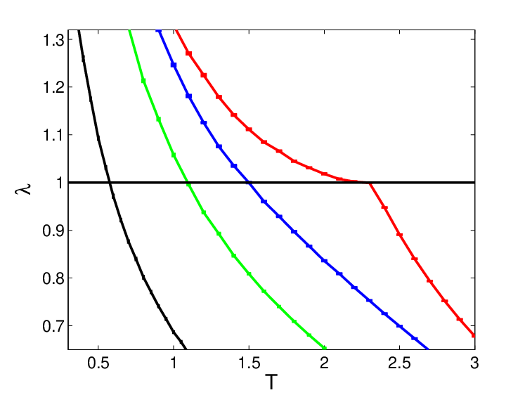
The behaviour of the stability parameter $\lambda$ can be studied analytically in zero external field close to the critical temperature. Writing $\tau=1-T/T_{c}(\alpha)$, one must compute the second and fourth moments of $P(h)$ up to order $\tau^{2}$, and then expand the eigenvalue equation (). One finds after some work $\lambda=1+(\alpha^{2}/3)\;(T_{2}(\alpha)+2T_{4}(\alpha))/(T_{2}(\alpha)-T_{4}(\alpha))\;\tau^{2}+O(\tau^{3})$, where $T_{n}(\alpha)=\int_{0}^{\infty}\alpha dx/x^{1+\alpha}\tanh^{n}x$. As the coefficient of $\tau^{2}$ is positive for all $\alpha\in]1,2[$, the RS solution is always unstable close to $T_{c}$, contrary to what was found with the Gaussian Ansatz [1]. The same is obtained numerically in presence of an external field : we have not found any evidence for a stable RS spin glass phase, at all the values of $\alpha$ and $h_{\mathrm{ext}}$ that we have studied.

To summarize, we have shown how the Lévy spin glass problem can be studied naturally within the framework of diluted spin glasses, using a decomposition of the couplings into strong and weak. The resulting phase diagram is very similar to the one found in other mean field spin glasses. In particular, the spin glass phase is never replica symmetric. The large fluctuations due to the presence of rare strong couplings request the introduction of some rather sophisticated methods in order to compute the spin glass instability. These fluctuations are even more pronounced in the case $\alpha<1$ not treated here where the free energy ceases to be self-averaging. They will also complicate the discussion of the RSB solution of the Lévy glass.

Acknowledgements : We would like to thank Martin Weigt for interesting discussions. Financial support from the Deutsche Forschungsgemeinschaft under EN 278/7 is gratefully acknowledged. MM thanks the Alexander von Humboldt foundation. While we were writing up this work, the preprint [15] has appeared where similar issues were addressed.