Towards Plugging Privacy Leaks in Domain Name System
Abstract
Privacy leaks are an unfortunate and an integral part of the current Internet domain name resolution. Each DNS query generated by a user reveals – to one or more DNS servers – the origin and target of that query. Over time, a user’s browsing behavior might be exposed to entities with little or no trust. Current DNS privacy leaks stem from fundamental features of DNS and are not easily fixable by simple patches. Moreover, privacy issues have been overlooked by DNS security efforts (i.e. DNSSEC) and are thus likely to propagate into future versions of DNS.
In order to mitigate privacy issues in current DNS, this paper proposes a Privacy-Preserving Domain Name System (PPDNS), which maintains privacy during domain name resolution. PPDNS is based on distributed hash tables (DHTs), an alternative naming infrastructure, and computational private information retrieval (cPIR) [14], an advanced cryptographic construct. PPDNS takes advantage of the DHT’s index structure to improve name resolution query privacy, while leveraging cPIR to reduce communication overhead for bandwidth-sensitive clients. Our analysis shows that PPDNS is a viable approach for obtaining a higher degree of privacy for name resolution queries. PPDNS also serves as a demonstration of blending advanced systems techniques with their cryptographic counterparts.
1 Introduction
Domain Name System (DNS) [22] is a global hierarchically distributed database. It translates human-readable hostnames into numerical identifiers associated with network-layer IP interface addresses for the purpose of locating (and routing to) individual hosts. Given the importance of DNS, much effort has been put into the next generation of secure DNS, referred to as DNSSEC [19]. The main purpose of DNSSEC is to authenticate the origin, and guarantee the integrity of, DNS records. Notably, DNSSEC explicitly rules out data disclosure threats [9].
It is easy to see that today’s DNS provides no privacy. All DNS messages are transmitted in the clear. A malicious local name server that delegates DNS queries for all clients in its administrative domain can easily gain all origin-target information. It also knows each target’s query volume from its administrative domain. Each name server in the DNS zone hierarchy – from the root to the authoritative server for a target queried by a local name server on behalf of its client – learns both the target of the query and query volume for the target. Although caching at the local name server hides the exact volume from other name servers in the hierarchy, authoritative servers can still infer expected query volume based on the distribution of queries’ arrival. Different leaks of DNS query pose differnt risks.
Leaks of query target’s identity can be abused for censorship purposes. For example, an ISP can forbid access to a host by simply dropping all queries for that host-name at the local name server controlled by that ISP. This approach, known as DNS filtering, is effectively employed by Great Firewall of China [2] to filter out websites considered as a threat by the state. Also it is part of the upcoming German national ISP filtering plan and similar efforts by Australian and New Zealand governments are already partially deployed. Although this is not the only way for an ISP to block a host, it is more effective than other approaches. First, a host name is easier memorizable than an IP address; hence, most people prefer to use host-names. Second, IP blocking may not work if a host can have a large pool of IP addresses and frequently change the mapping between its host-name and an IP address unknown to the ISP. If there was a perfect scheme for privately resolving host-names, the only conclusion the ISP would draw is that there is traffic between the client and an unknown IP address11 1 Assuming IPSec [19] can be used to hide all information above IP layer.. Of course, the ISP can use reverse DNS to retrieve the host-name corresponding to the unknown IP address. However, a host can simply configure its PTR record to some random name to prevent the ISP from learning anything useful. Another approach ISP can use is to install a proxy bound to all sensitive host names, hoping to catch all traffic directed to those host names. However, DNSSEC can effectively prevent this from happening.
Leaks of target query volume can be used for surveillance purposes. For example, if a DNS server observes a sudden spike in the number of DNS queries for a given host-name, it can alert authorities to check whether suspicious or offensive information on that host is causing its increased popularity. This is a common surveillance skill used in countries such as China to check possible sensitive websites.
Leaks of relative target query volume (which maybe inferred from target query volume) can be abused for commercial purposes. For example, suppose that the adversary can measure the relative popularity of any two domain names registered under a certain registrar. Then, the adversary might steal a popular domain name when its owner fails to renew it. One may think the chance is quite low for a popular domain owner to forget to register its domain name. However, in history, even industry giants like Microsoft once forgets to renew its domain names [5]. Many registrars have been making it more difficult for such theft to occur with auto-renewals, e.g., by parking domains for a grace period. However, if the adversary happens to be the registrar itself, it can reserve any popular domains registered under it and sell them at higher prices later.
Moreover, leaks of information during DNS query also pose risk to applications which rely on DNS as an underlying mechanism. For example, ENUM [13] (Telephone number mapping) system uses special DNS record types to translate a traditional telephone number into a Uniform Resource Identifier from VoIP providers, as well as to other Internet-based services such as E-mail and web page. The exposure of DNS query means the revealing of one’s daily contact list, which is considered to be a serious privacy betrayal.
This paper focuses on adversaries at DNS servers. It is true that a malicious DNS server can pose more threats than those mentioned above. We limit the scope of threats here based on the assumption that a powerful adversary does not want to expose itself too early by performing too aggressively. Although the above-mentioned leaks of information maybe collected by adversaries through other means, for adversaries at DNS servers, learning that information through DNS is a straightforward way. This paper focuses on addressing target-related DNS query privacy problems by proposing a privacy-preserving domain name system (PPDNS). PPDNS combines the use of a distributed hash table (DHT) with a computational private information retrieval (cPIR) [14] technique. Owing to consistent identifiers offered by DHT, the same range query can be posed for each identifier inside the range even in the presence of an active adversary, thereby hiding the actual query target. Moreover, we can also achieve the same range query for each identifier inside the range among all clients, thereby hiding the volume and relative volume for a query target. Furthermore, each DHT node can treat each range as a small database and take advantage of cPIR which allows a client to retrieve a record from a server (without revealing which record is being retrieved) with less than communication overhead; where is the number of database records.
The contribution of this work is as follows: (1) we investigate and categorize DNS privacy leaks, (2) we propose a novel range query technique that mitigates privacy leaks, (3) we design a flexible and parallelizable framework for incorporating cPIR at the server side, and (4) we provide a security analysis showing that PPDNS offers appreciably better privacy than prior work.
The rest of this paper is organized as follows: Sec. 2 provides an overview of current DNS. Sec. 3 formally defines the adversary model. Sec. 4 analyzes some existing approaches and explains why they are insecure. Sec. 5 introduces some preliminaries before presenting PPDNS. The architecture of PPDNS is given in Sec. 6. Detailed security analysis comes in Sec. 7. Sec. 8 shows the performance of PPDNS and Sec. 9 concludes the paper.
2 DNS Overview

The DNS [22, 23] namespace has a tree structure where each node, except the root, has a non-empty label. Each domain is a node in the namespace tree, and bottom-up concatenation of nodes’ labels delimited by periods (“.”), creates a fully qualified domain name. For instance, www.example.com is a fully qualified DNS name of a node www with the parent example, grandparent – com, and great-grandparent – DNS root.
Nodes are grouped together into zones. The apex of a zone is called the start of authority (SOA) and bottom edges are called delegation points if other zones exist below them, or leaf nodes, otherwise. Zones are served by authoritative name servers that are either primary, if the zone data comes to them from the outside of DNS, or secondary, if their zone data comes to them from primary servers via a zone transfer procedure. Authoritative name servers manage all name information in the domain, keep track of authoritative name servers of their sub-domains rooted at their domain, and are administered by namespace operators.
Every node can store resource records (RRs) containing information associated with a domain name. A RR can map a host name to an IP address or vice versa, or serve a variety of other purposes. Each RR has a name, class, type, TTL and data. A RRset is a list of all the records matching a given domain name and resource type. A nameserver returns a RRset as a response to a query.
DNS initiators on host machines are called stub resolvers; they do not have caches of their own and do not directly interact with the zone hierarchy. They pose basic queries to local name servers, also known as recursive resolvers, within their own administrative domain. The local name server is usually designated by the ISP and only provides service to hosts within its administrative domain. It accepts recursive queries from stub resolvers, contacts a chain of authoritative name servers inside the zone hierarchy to locate a DNS RRset, and answers the stub resolver. Because pursuing a chain of delegations to resolve a query can incur significant delays, the local name server caches the result and answers subsequent queries using the cache, until a TTL (assigned by the authoritative nameserver) expires.
In an example shown in Fig. 1 (which assumes no caching), the resolution of www.example.com involves following steps: (1) The user types the domain name into the web browser which consults its local stub resolver, usually implemented as a set of library routines. (2) The stub resolver sends the query to its local name server. (3) The local name server consults with the root server – the authority for the empty label. (4) The root server refers the local name server to “com.” zone’s authoritative server. (5) The local name server consults a “com.” zone’s authoritative server. (6) It delegates the local name server to “example.com” zone’s authoritative server. (7) The local name server consults “example.com” zone authoritative server. (8) This authoritative server answers the host address record for “www.example.com”. (9) Finally the local name server caches the resource record and meanwhile returns the result to the stub resolver. (10) The stub resolver returns the IP address to the web browser which then launches connection to the IP address.
3 Threat Analysis
In this section we discuss DNS privacy threats and the adversarial model.
3.1 DNS Privacy Leaks
We consider the following DNS privacy leaks/problems:
- 1.
query source-target association
- 2.
query source identity
- 3.
source query volume, i.e., number of DNS queries issued by a given source.
- 4.
relative source query volume, i.e., the difference between query volumes for two given sources.
- 5.
query target identity
- 6.
target query volume, i.e., number of DNS queries issued for a given target.
- 7.
relative target query volume, i.e., the difference between query volumes for two given targets.
Of course, DNS clients may choose to use a general-purpose anonymization service, such as TOR [12] to hide the DNS query source. This prevents problems (1)-(4). However, source anonymity afforded by tools like TOR does nothing to address target-specific leaks (5)-(7). In the rest of this paper, we focus on the latter.
3.2 Adversary Model
An adversary can be an insider or an outsider. Outsider is an adversary that does not compromise any name server and only eavesdrops on messages to learn target-related information in the DNS query. We are not interested in this type of adversary, since standard security tools, such as SSL/TLS and/or IPSec [19], are effective against them. Insiders refer to malicious local or authoritative domain name servers. Although a malicious local name server can be trivially bypassed by letting clients running their own recursive resolvers, we still need to seriously analyze the malicious local name server’s advantage given the fact that few clients are willing to sacrifice the performance gained from caching at the local name server. Insiders can be further classified into:
- 1.
Passive (Honest-but-Curious) Insider - only listens to queries sent to it but responds honestly.
- 2.
Active Insider - may drop, forge or manipulate DNS responses.
We further assume that malicious name servers under the same namespace operator’s control may collude.
3.3 Advantage of the Adversary
We now formally define the advantage of the adversary . First, we give some definitions. denotes the average number of queries for name within time interval . We give different meanings based on where it is measured. At a local name server, represents the number of queries only from its local administrative domains, while, at an authoritative name server, represents the number of queries from all over the world.
The advantage of a specific in terms of each privacy leak in Sec. 3.1 is defined to be:
- 1.
: the probability of successfully outputting the target identity for a query against domain name .
- 2.
: the probability of successfully outputting for a given domain name .
- 3.
: the probability of successfully outputting for two given domain names and .
In the following, we may omit the parameter and use for simplicity.
4 Privacy Threats with Existing Approach
It is easy to see that, in current DNS, all three advantages in Sec. 3.3 are for the respective insider adversaries. In this section, we discuss some existing approaches that attempt to mitigate the situation.
4.1 General-Purpose Anonymity Service
TOR [12] uses the onion routing technique to hide traffic source. As mentioned earlier, it is an effective approach for hiding the source/target relationship, query source, source query volume and relative source query volume. However it has nothing to do with mitigating target-related leaks.
4.2 Random-Set Query
Zhao, et al. [31] and Castillo-Perez, et al. [10] propose a random-set query approach. Specifically, each time a client queries a domain name , it constructs a query set , of size , comprising of (real target) and randomly picked names (confusing targets). The source then queries each of the names. This method has the advantage of easy implementation and requires no changes to current DNS infrastructure. However it has some notable drawbacks.

With respect to , both [31] and [10] claim their respective approaches can achieve . However, this is not necessarily true in the face of an active malicious local name server that can force a client in its administrative domain to re-launch a random-set query to the same target. A local name server can achieve this (while remaining undetected) by simply dropping requests from a local client within a short period of time. Let denote the random set of the th query to target . If the local DNS server can get random set queries for the same target, , then, since , instead of . Let denote the pool of domain names where the client picks both the real target and the confusing targets. Let denote the size of . For each name , the probability of appearing in is . Therefore, the probability of is assuming that confusing targets are independent for each . Thus, the average size of the intersection is . Fig. 2 gives an example of the relationship between and . It shows that, as increases, increases dramatically, especially, when is small.
As far as is concerned, at the local name server still has full advantage. Assume that , within the past interval , witnessed domain names being queried. counts the number of queries from its administrative domain to in interval as which includes both queries for as real targets and those querying as confusing targets. Let . Then where is the number of queries which query as a real target. For each , its confusing targets have probability of hitting for . Therefore, we have:
Solving this equation yields .
We also observe that for both malicious local name servers and authoritative name servers. It is trivial for at a local name server to compute , since it already knows and (). If is an authoritative server, it does not learn , since it does not know and . However, , given . Thus, can also easily determine .
4.3 Fixed-Set Query
Instead of choosing confusing targets randomly, each client can fix them for each real target . This can be achieved efficiently through a pseudo-random function with a seed only known by the client. This way, each query for the same target will end up with the same set and . However, this approach lacks robustness. If the adversary learns the mapping of a target from one client, all future requests for from that client is clear to the adversary since the mapping is fixed. Moreover, for a malicious authoritative name server, is still . This is because it is hard to synchronize the mapping function between different clients and therefore the fixed set chosen for the same target by different clients are still independent. If in time , the number of requests to or from the same client is negligible to the total volume, then still gives a good estimate of for the same reason as discussed in Sec. 4.2.
4.4 Combining Tor and Random Set Query

If we combine Random-Set Query with TOR, the adversary at the local name server cannot force the same client to relaunch a random-set query to the same target. As shown in Fig. 3, a client can use TOR to query “local” name servers around the world by forwarding random-set queries to TOR nodes in different regions. This way, an adversary at a single local name server cannot see multiple random-set queries to the same target by dropping client’s requests, since if a random-set query is dropped, the client can choose a different local name server to relaunch the query. As long as there are honest local name servers, the client’s query can be answered. This approach effectively reduces to for adversaries at local name servers. However, this gain does not come for free. To maintain perfect unlinkability, the client needs to create a new TOR circuit, which can take more than seconds [24], for each DNS query. This is a very high overhead for a client that only wants to hide its query target. Also, if the number of TOR users in a local domain is negligible, and for adversaries at local name servers remain quite high. Moreover, even there are large number of TOR users, for adversaries at authoritative servers is not affected, since they are the ultimate “sink” for all queries.
4.5 DNS Caching
DNS caching only moves the overhead of DNS resolution from authoritative name servers to local name servers. Thus, as pertains to at a local name server, caching does not offer any privacy benefits.
With caching, if is located at an authoritative name server, it cannot learn the exact query volume for a target. However, it can still compute the average target query volume. To see this, we first need to model the arrival process of DNS request. Poisson processes are widely used to model events if times between consecutive events are independent random variables and the number of events in one interval is independent from previous intervals. Earlier work [25] suggests that session inter-arrivals can be reasonably approximated by an exponential distribution, and that has been supported in studies on DNS caching [16]. We thus consider it reasonable to model DNS requests’ arrival events as a poisson process.
We assume the arrival process of DNS queries to target from a local administrative domain conforms to a poisson distribution with arrival rate . Let denote the TTL for . After a client within a local administrative domain queries its local name server for , the local name server caches the response (from authoritative name server) for time . After seeing a query against from a local name server from domain , the adversary knows that, within the next period of length , it will not see further queries from this local name server. However, because of poisson distribution, knows the average number of queries against in the following time is . Given a longer time period , can count the number of queries, , against from the local name server. Then, it can estimate the total number of queries that occur in time as: . Again, due to poisson distribution, the following equation holds:
Solving it yields and as the average number of queries from that local administrative domain . Finally, summing up the average number of queries from all local domains, obtains .
If is an active insider at an authoritative name server, it can also set the TTL to a negligible value, since it has the right to do so. Then, retains the same advantage as discussed in previous sections.
4.6 Information-theoretic Private Information Retrieval
Information-theoretic PIR is a cryptographic technique that allows a client to retrieve a record from two or more non-colluding servers, each having a copy of the database, without either server learning which record the client wants to retrieve. Zhao, et al. [32] use the two-server version of information-theoretic PIR to achieve DNS query privacy. However, information-theoretic PIR requires the assumption of multiple non-colluding servers, each having a copy of the database. In reality, servers with duplicate database are usually the primary and secondary servers for the same zone. These servers can collude with each other according to the assumptions in Sec. 3.2, since they are under control of the same namespace operators. Thus, we do not consider information-theoretic PIR to be suitable for preventing leaks in DNS queries.
5 Building Blocks
In this section, we introduce some building blocks that are used in our system.
5.1 DHT-based DNS
Distributed hash tables (DHTs) are a class of decentralized distributed systems that provide a lookup service similar to a hash table: (key, value) pairs are stored in the DHT, and any participating node can efficiently retrieve the value associated with a given key. There has been plenty of research devoted to flat-structure DHT-based DNS [26, 11]. In fact, some results have already seen trial deployment on the Internet. DHT-based DNS solutions propose to use a flat-structure to replace the current hierarchical DNS structure. Basically, it is a peer-to-peer domain name system wherein both nodes and objects have randomly assigned identifiers from the same circular space. Here we take CoDoNS [26] as an example and describe its architecture in detail.
CoDoNS is based on prefix-matching DHT. It designates the node whose identifier is closest to the consistent hash of a domain name as the home node for that domain name. The home node stores a permanent copy of the resource records owned by that domain name and manages their replication. If the home node fails, the next closest node in the identifier space automatically becomes the new home node.
CoDoNS supports DNSSEC by separating the authentication of data from the service of that data. Every namespace operator has a public-private key pair; the private key is used to digitally sign DNS records managed by that operator, and the corresponding public key is in turn certified by a signature from a domain higher up in the hierarchy. This process creates a chain of certificates, terminating at a small number of well-known public keys for globally trusted authorities. The signature and the public key are stored in CoDoNS as resource records of type sig and key respectively. Clients can verify the authenticity of a resource record by fetching the sig record and the key record from the CoDoNS. CoDoNS servers cache the certificates along with the resource records to help clients check the validity of a record.
CoDoNS decouples namespace management from the physical location of name servers in the network. Namespace operators do not need to participate in the data serving. Their responsibility is only to sell certificates of names they account for to nameowners. Nameowners later introduce these names into CoDoNS. CoDoNS servers authenticate nameowners directly through certificates provided for every insertion, deletion and update. CoDoNS is agnostic about the hierarchical structure of namespace while namespace operators are agnostic about which CoDoNS servers are serving the names they give a certificate to.
Some common DNS operations are not specified by CoDoNS but can be easily combined into any DHT-based DNS. For example, to support wildcard query, a DHT node, when finding unmatched result for a specific subdomain name, e.g. “random.example.com”, the DHT node can redirect this request to a node accounting for ”*.example.com” where there is a record for default mapping.
5.2 Gentry-Ramzan(GR) cPIR
Gentry-Ramzan cPIR [14] is a computational private information retrieval (cPIR) scheme. cPIR schemes typically assume a single server, in contrast to multiple non-colluding replicated servers required by information-theoretic PIR.
In Gentry-Ramzan (GR) cPIR, the database server and clients share distinct prime numbers , and prime powers where and for a database with blocks, each of size at most . Each block is associated with a prime power . Using the Chinese Remainder Theorem, the server can express the entire database as an integer that satisfies . Notice that to retrieve , it suffices to retrieve since .
Query Generation: The user determines index of its desired block, and then generates an appropriate cyclic group with order for some suitable integer . It sends to the server and keeps private. It also stores for future use. Note that is a generator of subgroup of order .
Database Response Generation: The database server first expresses each block as a number in in the obvious fashion. Then it sets to be the smallest positive integer such that for all by Chinese Remainder Theorem. Last it outputs the response to the user.
Response Retrieval: Given the input , the user retrieves block as follows: It computes and gets through the discrete logarithm within the subgroup of order using Pohlig-Hellman algorithm.
To instantiate the cyclic group , one may first construct a random “semi-safe” prime for some prime and a random safe prime for some prime and set as a composite modulus. Then one can take a quadratic residue from and test if it is a generator for a cyclic group whose order is which is where is Euler’s totient function until a generator is found.
The security of this scheme comes from -Hiding assumption that it is computationally intractable to decide whether a given small prime divides where is a composite integer of unknown factorization. In other words, given a cyclic group constructed in above way where , the server is computationally difficult to test which divides and therefore computationally difficult to know which element the user tries to retrieve.
6 PPDNS Architecture
This section describes the Privacy Preserving Domain Name System (PPDNS) which aims to mitigate target-related DNS privacy problems. PPDNS is built upon a DHT-based naming infrastructure. It takes advantage of DHT’s index to implement fixed-range routing. It also offers bandwidth-limited clients the option of using cPIR to reduce communication overhead.
6.1 Why DHT-based DNS?
Having examined existing approaches, we conclude that current DNS cannot be amended to offer privacy due to its fundamental design features. Therefore, we must consider new approaches for emulating DNS that would lend themselves to better privacy. We believe that DHT-based DNS is a viable candidate for a privacy-preserving domain name system.
There are two privacy advantages of DHT-based DNS. First, it uses consistent hashing for object location, which enables approaches, such as fixed range query and cPIR. Second, the flat and balanced storage structure gives equal power to adversaries compromising different servers. This is in contrast to adversaries in current DNS that attain more power by compromising higher-level DNS servers or servers with more records.
6.2 Why GR cPIR?
There are many available cPIR schemes. Our choice of GR cPIR is based on two factors. First, its communication complexity is , where is a security parameter that depends on the database size and is the bit-length of the retrieved database block. This communication complexity is, by far, the best. Second, the dominant component of server’s computation is in computing which consists of at most modular multiplications, where is the number of blocks in server’s database and is the block length. As shown in Sec. 8.2 below, this amount of overhead can be tolerable for DNS servers in some circumstances.
6.3 PPDNS protocol
We begin by introducing some definitions and notation. All clients and PPDNS nodes share a hash function that maps any domain name into a circular space where is the upper-bound of the hash space. We use SHA1 [8] as the hash function, and thus, . We say that an identifier is empty if there are no domain names attached to it. We refer to the identifier space density as – the ratio of the number of non-empty identifiers to the total number of identifiers. Each PPDNS node can compute individually, due to the uniformity of the hash function. We define query range for a target identifier to be a set of continuous identifiers, including the target identifier. We refer to the identifiers in the query range – except the target – as confusing identifiers. Each client has a security parameter representing the number of non-empty identifiers it expects in the query range.
Each client gets its estimate of from its local name server and periodically updates it as a moving average of its previous estimate and newly learnt values. A client who wants to resolve a target domain name first hashes it into an identifier . Then, it determines the number of non-empty identifiers, , in its query range. The actual range size is computed as where . We expect most clients to have the same and . However, we allow clients to have different -s and have some estimation error on . The reason for the client to select its range as a power of is to accommodate these differences. Finally the query range for target identifier is formulated as:
| (1) |
Theorem 7.1 shows that, if the query range is formed in the above manner, then the query range generated for each identifier is fixed and the same query range can be posed for each identifier inside this range. Theorem 7.2 shows that, even for clients with different and values, the intersection of their query ranges is guaranteed by the smallest query range among them.
Next, the client constructs a range query, which only needs to include the start and end identifiers. The range query is initially sent to the local PPDNS node which replies immediately if it has a cached copy of the queried range. Otherwise, it routes the query towards its destination node, which accounts for the identifiers inside the range, by following the underlying DHT protocol. If any intermediate PPDNS nodes happen to have a cache of the queried range, they respond directly to the local PPDNS node and the query stops. Otherwise, they pass the query onto the next intermediate node until it reaches the destination.
Range splitting may occur and multiple sub-range queries may be generated at intermediate PPDNS nodes. A PPDNS node that has complete records for a sub-range query returns all records (with identifiers inside the subrange) to the local PPDNS server. The local PPDNS server waits until all responses arrive and then delegates them to the client. The local PPDNS server also caches the whole range of responses for the minimum TTL among all responses in the range. Since all clients in the same administrative domain get from the same local name server, they come up with the same range size, as long as is also the same. Therefore, by caching the whole range answered to one client, the local PPDNS server can also answer later queries from other clients.

As an example, consider Chord [29] circular space shown in Fig. 4 where . Suppose the client wants to query a domain name with hash identifier . Then the client will make a range query of according to Eq. (1) to its local PPDNS server (node ). Node forwards this range query to node by looking at its finger table. Node further forwards the range query to node which is the home node for range . Node first splits the range into and . Then it replies the records corresponding to range to the local PPDNS server and further forwards the subrange query of to node which later replies to the local name server with records corresponding to range . The local name server finally delegates the answer to the client.
6.4 cPIR support

As an option, the client may choose to use cPIR to save bandwidth. Modern residential ISPs can offer up to Mbps download speeds; thus, most clients do not need to worry about the extra communication overhead due to range queries. However, for GPRS [3] users in developing countries, the maximum currently achievable speed is between and kbps, depending on the distance to the base station. If we assume the user issues one range query with every seconds, the bandwidth tallies up to kbps for regular DNS ( bytes per response) and kbps for DNSSEC ( bytes per response), which consumes a lot of the channel’s capacity. This is unacceptable for most GPRS users. Moreover, many cell phone users’ data plans are based on traffic volume, especially, when roaming in foreign countries. These factors motivate the use of cPIR.
To take advantage of cPIR, the client needs to view the query range as a small database. An output of a secure hash function is typically on the order of hundreds of bits (e.g. 160 for SHA-1). The total number of domain names with respect to the total number of identifiers in the hash space is quite low, i.e., is very small. Given the low density of the hash space, simply using the hash identifier as the index into the database for cPIR would work. However, it would cause very high computation and bandwidth overhead as cPIR’s overhead is proportional to the number of database entries.
One way to tackle this problem is for the client to divide the range (database) into equal blocks and assign a consecutive index to each. Then, the client uses cPIR to retrieve the block which contains the desired identifier’s record. Because the hash function is near-uniform, the average number of non-empty records in each block is . This way, cPIR overhead is proportional to instead of .
Consider an example in Fig. 5 where hash output is bits and . A client picks a query range (3b0000-3bffff). It wants to retrieve the blue record with identifier 3b5a5c but it does not know the other non-empty identifiers. If the client sets , the whole range is split into two equal-size blocks and, by reassigning the blocks, it knows that the blue record lies in the first reassigned block which accounts for identifiers from to 3b7fff. Next, the client retrieves the first reassigned block, which includes three original records from the server. The choice of depends on the computation power of the server, which is to be analyzed in Sec. 8.2. The larger is, the lower the communication overhead is while the higher the computation overhead is. Any cPIR schemes can fit here. Due to the reasons we explained in Sec. 6.2, we currently employ GR cPIR in PPDNS. In the future, however, if there are more efficient cPIR schemes, we can easily apply them here.
In order to incorporate GR cPIR, we need the local name server and the clients to share a sequence of consequtive prime numbers. The number of prime numbers should be equal to the maximum number of blocks the local name server allows a client to retrieve each time. When the client issues a range query, it also indicates a range of prime numbers. The client can do so by only showing the ending prime numbers’ index in the consecutive prime numbers’ list if the client always use the first prime it shared with the server as the starting prime. From the range of primes embedded inside the range query, the server can compute the number of blocks the client wants to divide the range into. Then, the local PPDNS server gets all the responses to this range from other servers (through normal range query described in Sec. 6.3) and then performs cPIR with the client. If the local PPDNS server happens to have cached the whole range, it can perform cPIR immediately.
Currently, we only employ cPIR between the client and the local PPDNS server. If cPIR was also used between PPDNS servers, the range cache would be no longer possible. We observe through simulation in Sec. 8.3 that the cache captures more than % of all range queries. Thus, giving up the cache actually counteracts cPIR benefits. Moreover, due to the high capacity of backbone links, backbone traffic resulting from a range query is very limited (less than % in our simulations). Therefore, we see no reason to use cPIR between PPDNS servers.
As an example in Fig. 4, if the client chooses to use GR cPIR and decides to divide the range into blocks (), it indicates its prime range by sending the prime index along with its range query , which means using the first eight prime numbers in the consecutive prime number lists shared with the local name server to execute GR cPIR. When the client receives the answer to the query range , it knows its desired index can be extracted by using the th prime number in the shared prime number lists.
6.5 Other Ideas
To facilitate incremental deployment, the client relies on current DNS to resolve queries for records not in PPDNS and explicitly inserts them into the system. To protect its privacy from adversaries in both DNS and PPDNS, the client first queries PPDNS with the range formed by Eq. 1. Once client realizes the target domain name’s RR set is not inside the response, it uses the same range query to query current DNS. Instead, the domain names except the real target inside the range query to current DNS is learnt from the responses of PPDNS. Once the client learns the records for target domain name, it asks a random PPDNS node (e.g., chosen by random walk [15]) to insert the target into the system. DNSSEC is employed for preventing poisoning attack.
7 Security Analysis
In this section, we analyze the security of PPDNS in terms of adversary’s advantage described in Section 3.3.
First, we state two theorems about range selection in Eq. 1. In short, the first theorem states that the query range for a specific identifier is fixed, such that the same range can be formed for each identifier inside this range. The second states that even if clients have different and values, the size of the intersection of their ranges for the same identifier cannot be smaller than the smallest range size among them, which gives the adversary limited power by making intersection over query range.
Theorem 7.1
such that divides N, the query range generated by Eq. (1) for any identifier is fixed and the same query range can be posed for any identifier inside this range.
Proof
Suppose . Then, for any identifier , there exists one such that . Moreover, , the range generated by Eq. (1) for is .
Theorem 7.2
The lower bound of the size of the intersection for all query ranges generated for a common identifier by different clients with different and is guaranteed by the smallest .
Proof
We only need to prove that, if two ranges: and where , overlap, then .
If , then . Since both sides are integers, we have . Therefore, . Similarly, we can prove that if , then .
Thus, if one end of falls inside , so does the other. Then, the theorem holds.
We expect that most clients have the same security parameter . As to be shown in Sec. 8.1, the density estimated at different PPDNS node in real senario is very close. These facts combined with Theorem 7.2 means the intersection size should be reasonably close to . Even if some clients use extremely small , it only affects as to its own query and has limited effect on and as long as the number of such clients are small.
Now we use the model of Sec. 3 to analyze the security of PPDNS. We assume all clients have the same and parameters. Recall that any PPDNS server can be both a local name server and an authoritative name server. We neglect the security analysis for intermediate routing PPDNS nodes, since their advantage is captured by the authoritative name server.
A passive at a local PPDNS server receives range queries from, and provides responses, to clients in its administrative domain. By examining range responses that it delegates to clients, it knows all domain names inside the range. Therefore, .
As far as target volume, suppose that is the total volume for target ’s query range from the local administrative domain. Then, the average volume to should be , where is the probability of being queried in each range query to . If we assume does not have any prior knowledge of , any value from to is equally likely, from ’s perspective. Therefore, the target volume can be any value between and and .
One issue may come into mind is that if the confusing identifiers have low probability and the real one has high probability, a plaintext attack is possible since hash value is fixed for each identifier. However, we think this kind of difference between confusing and the real identifier comes from prior knowledge before PPDNS is deployed. Once PPDNS is fully deployed, the prior knowledge would become less and less credible over time.
In terms of relative target volume, given two domain names and , if the total volume to and is and respectively, then, in ’s view, can be any value between and . Therefore, . Note that and only relies on the volume and has nothing to do with query range . In particular, if (resp. ), (resp. ).
An active at a local PPDNS server can drop a response without being detected. However, this does not give it more advantage, since the same range query is always issued for the same target, as shown in Theorem 7.1. has no incentive to spread false density information to clients in its administrative domain, as doing so can be detected by checking the density difference with other PPDNS nodes. also has no motivation to forge or manipulate responses since DNSSEC can effectively prevent this. Therefore, the advantage for the active malicious local DNS server is the same as that of its passive counterpart.
A passive at an authoritative PPDNS server knows whether an identifier in its charge is empty or not, since . The advantage of guessing target query volume is again , where is the total volume to the target identifier’s query range. And, the advantage of guessing relative target query volume is if , where is the volume to two given domain names’ query range.
An active at an authoritative PPDNS server cannot change the TTL or manipulate RRset, unlike an authoritative name server in today’s DNS, since all records are signed by different namespace operators and the authoritative PPDNS server is just a host for domain names for which it does not have corresponding signing keys. Thus, its advantage is the same as that of a passive adversary.
8 Performance Evaluation
This section evaluates the performance of different components comprising PPDNS.
We start with judging the accuracy of computing density , which plays an important role in determining query range. Then we benchmark a cPIR scheme, an optional feature supported by PPDNS, to see how much bandwidth it can save a client and how much computation power it would take. Last, we test PPDNS’s performance under realistic backbone environment through simulation.
8.1 Density Estimation Accuracy
Density estimated at each PPDNS node plays an important role in determining the query range Eq. 1. Recall that clients in the same administrative domain have the same estimated , since they all get it from the local PPDNS server. However, there is a security threat if values estimated at different PPDNS nodes vary significantly. This is because: (1) large deviation in allows the local adversary to cheat clients by spreading larger , which may not be detected and (2) by intersecting query ranges, may gain higher advantage, since the intersection size is the smallest query range for a specific target identifier.
SHA1 is well known for maintaining uniformity across its space. However, due to the importance of , we want to make sure SHA1 can maintain high uniformity in terms of domain names as input. To test this, we retrieved all the second-level domain names ending with “.com” ( total) from VeriSign [7] in July 2009, prefixed each with “www.”, hashed with SHA1 and stored these results at Chord Nodes.


Fig. 8 shows the density deviation with respect to the number of PPDNS. Errorbars show quantiles 5, 50 and 95 related to the set of density estimation made at each node. As we can see, the deviation of density estimation increases with the number of nodes. This is expected because, with more nodes, the sample space at each node becomes smaller.
To measure the range deviation, we set to be for all nodes and check the deviation of which is the logarithm of the final range size to the base of two. We choose a large here because larger tends to generate larger error. Fig. 8 shows the range deviation. The errorbars here capture the minimum, median and maximum points. As we can see, until the number of nodes reach , the estimated at each node is exactly the same. Even when the number of nodes is equal to , the difference of the maximum/minimum with the median is only . We expect in the real world, the number of domain names will be much bigger and the error will be even smaller.
8.2 Performance of GR cPIR
Storage Overhead
With GR cPIR, all clients and servers need to synchronize a list of prime numbers, the number of which decides the maximum number of blocks a client can retrieve from the server. This can be easily achieved by sharing a range of consecutive prime numbers. Theoretically, there is no limit to the number of shared primes. But, in practice, since is good enough for hiding clients’ target, storing one thousand prime numbers are enough. Therefore, the number of shared primes would not pose a serious overhead for the client and the server.
Communication Overhead
The advantage of GR cPIR is its near-optimal communication overhead. Specifically, the communication from the client to the server includes one index indicating the ending prime number in the shared list, the generator of a cyclic group and a composite modulus. The communication from the server to the client is just a group element. For example, if we set the modulus to be bits, we can safely retrieve a block of length bits from a database of blocks. Then we have the generator, the modulus and the prime index to be bits, bits and bits respectively. The response from the server is bits. Therefore the total communication overhead is bits. If the block length bits, we can split each block into chunks with 512 bits each and execute instances of cPIR in parallel. Since these instances share the same generator and modulus, the client only needs to send the generator and modulus once. And the communication overhead becomes bits. This is an tremendous improvement over the communication, compared to trivially sending all the blocks whose communication is bits. Fig. 8 shows the compression ratio under different combination of and . As we can see, the larger or is, the higher the compression ratio is.
Computation Overhead


We implemented GR cPIR by using GMP library [4] and tested it on a desktop with Intel Core i7-920 (2.66MHz and 8M cache, MSRP: ) inside. We choose the group modulus to be bits long which is expected to be safe until 2030 [17]. As described in Sec. 5.2, GR cPIR includes three operations: (1) server representing the whole database as an integer through Chinese Remainder Theorem, (2) server responding to client’s query by modular exponentiation . (3) client computing discrete logarithm by Pohlig-Hellman algorithm.
Fig. 11 shows the speed of computing congruence by Chinese Remainder Theorem. We can see that computing bits congruence takes negligible time until reaches , where the time spent for bits is ms, which means real time congruence computation for is possible. We can also see that the computation overhead increases super linearly with the block size and with the number of retrieved elements . However, a local PPDNS node does not always need to do this operation on demand. If a local PPDNS server has a cache of the range of responses, it can precompute for this range to save time for future queries.
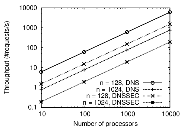
Fig. 11 shows the computation time of modular exponentiation . Since is a representation of the whole database, its size is up to bits. From Fig. 11, we can see that the speed of modular exponentiation is still quite slow. To retrieve blocks of bits each, it takes ms. The maximum size of a regular DNS response is bytes (k bytes for DNSSEC). In other words, to retrieve a DNS response, the worst time is ms for regular DNS (ms for DNSSEC). However, if we consider a server equipped with multiple processors, each -bit block retrieval can be executed in parallel, therefore it is possible to make this scheme scalable. These processors can be some cheap special-purpose FPGAs [21] which can work faster than general-purpose CPU in computing modular exponentiation. Fig. 12 shows the number of requests a server can serve in one second with respect to the number of processors it uses. From the figure, we can see that at least processors are needed to serve concurrent requests if we assume the server receives requests per second. This actually matches Sion’s results [27] that it is computationally expensive to deploy cPIR. However, as long as one is willing to invest money on the server side, cPIR can still be practical in reducing communication overhead.
Fig. 11 shows the speed of extracting the exponent from the response. As we can see, the time increases quadratically with and is stable for small . Retrieving -bit exponent takes up to ms for . However, the waiting time occurs only at the client side and it does not block other user’s response. A user who executes cPIR should be ready for some reasonable waiting time (several seconds).
In conclusion, GR cPIR works impressively well in reducing traffic between the client and the server. However, it also poses high computation overhead on both sides. Fortunately, we notice there are some high-speed efficient cPIR variants [30, 20] and we expect more efficient cPIR schemes to appear in the future. As PPDNS’s support for cPIR is flexible, we can accommodate any promising cPIR schemes into the system.
8.3 Simulation Results
In this section, we examine PPDNS’s performance through simulations built on NS-3 [6] and show that PPDNS can efficiently do target lookup while incuring reasonable cost to the backbone network.
We compare the average delay, maximum link utilization and cache hit ratio of PPDNS with standard single query and random-set query performed in DHT-based DNS. We also study the range split ratio in PPDNS.
Setup
We collected the DNS trace at one of UCI’s name servers between June and July 2009. We exclude those non-legitimate names by querying each distinct names in the trace, which results in distinct legitimate fully-qualified names. For each legitimate name, its TTL and response size are recorded. We feed each simulator node in NS-3 with one distinct day’s DNS trace from 12:00 pm to 22:00 pm. We choose Chord [29] as the underlying DHT for PPDNS. Each simulator nodes’ identifier is randomly picked from the hash space.
| Topology | Type | # of Nodes | # of Links |
|---|---|---|---|
| Abilene | R | 11 | 28 |
| Geant | R | 23 | 74 |
| Sprint | I | 52 | 168 |
| Tiscali | I | 41 | 174 |
| Brite-1 | A | 50 | 342 |
| Brite-2 | A | 50 | 386 |
We simulate PPDNS with backbone topologies as we expect that PPDNS should be deployed at domain level. We use real, inferred, and synthetic topologies in our simulations. For real ones we use the Abilene backbone topology and the Geant backbone topology. We also use the topologies inferred by the Rocketfuel project [28]. In addition, we generate synthetic topologies using the BRITE [1] topology generator. All real and inferred topologies are on the level of Point-of-Presenses (PoPs). Table 1 summarizes the topologies.
For real topologies, we use the actual link capacity in our study. For Rocketfuel and random topologies, the link capacities are set according to a two-tier model [18] where each link is either OC48 (i.e., 2.48Gbps) or OC192 (i.e., 10Gbps). Specifically, Links connecting to the top 20% PoPs with the highest node degrees have the higher capacity (10Gbps), while other links have the lower capacity (2.48 Gbps). In addition, we make each link’s initial utilization to be at to simulate a median loaded network. We set the propagation delay of the link with the smallest weight to ms and make all the other links’ delays proportional to their weights.
Maximum link utilization


Fig. 15 and Fig. 15 compares the variation of the maximum link utilization with time in the case of the random topology for our range query and random-set query. The line marked with means single query. We omit other topologies here because they all show the same trend. The link utilization we show here excludes the link’s initial load and is purely contributed by DNS queries. As we can see, the maximum link utilization almost doubles as the range size doubles. Our range-query scheme sees less maximum link utilization than random-set query.
To further compare the link utilization between our range query and random-set query, Fig. 15 shows the maximum link utilization averaged over time for different topologies where is fixed at . We can see that our range query is much better than random query in terms of maximum link utilization. This is due to the fact that the local PPDNS node has a high chance of caching the whole range if there is a previous range query to any target inside this range. While as to random-set query, even if the same target has been queried before, there is little chance PPDNS can cache all responses for every name inside the random set of a new query for the same target since the random set chosen each time is random.
Average Delay


The delay calculated here is caused purely by backbone network, not including the delay between end host and local PPDNS node. Fig. 18 shows the average delay for our range query. As we can see, the average delay in different cases is almost the same as a single query (e.g. ). This again is due to our range query’s better capability of being cached. We measure the delay for a random set query as the delay between when the first request is sent and when the last response is received for one query set. From Fig. 18, we can see the average delay for random-set query, is much higher than that for the single query and our range query.
Cache hit ratio
Fig. 18 shows the cache hit ratio for our range query. We can see that the cache hit ratio decreases first as query range size increases and then the ratio increases. This is because the TTL for a range is decided by the smallest TTL of all domain names’ TTL inside the range. By increasing the range, the smallest TTL has a chance to decrease and therefore the hit ratio decreases as well. However, further increasing range size also helps cache more results which increases the probability of the range being hit. That is why cache hit ratio at is higher than that at . Also we can see that the cache hit ratio is over for our range query in all cases. In contrast, the cache hit ratio for random-set query is zero throughout our study and we do not show it here.
Range split ratio

Finally, we measure the split ratio for the range query. Range split can cause extra response delay, since local PPDNS needs to wait for all split-ranges’ responses to arrive before answering its client. Fig. 19 shows the percentage of queries which are split in our study. In all cases we examined, the split ratio is below . And it is linearly proportional to query range size. We only use legitimate domain names in our simulation. If we increase the number of available domain names (up the density), the split ratio should decrease accordingly. In practice, we expect the total number of legitimate domain names to be 100 times larger than we recorded. Even with a range size of , the split ratio should remain below .
9 Conclusion
In this paper, we propose a new Privacy-Preserving Domain Name System, called PPDNS. PPDNS is built upon DHT and employs a special range query which takes advantage of DHT index structure to yield a secure system. Meanwhile PPDNS incorporates an adjustable cPIR framework which can help clients reduce their communication overhead.
Security analysis shows that PPDNS significantly improves privacy for name queries. Performance evaluation demonstrates that PPDNS incurs reasonable communication overhead to the backbone links. It also shows that PPDNS retains the efficient part of the traditional DNS–high cache hit ratio, and incurs much lower latency than random-set query.
References
- [1] BRITE Topology Generator. http://www.cs.bu.edu/brite.
- [2] Empirical analysis of internet filtering in china. http://cyber.law.harvard.edu/filtering/china/appendix-tech.html.
- [3] General packet radio service. http://en.wikipedia.org/wiki/General\_Packet\_Radio\_Service.
- [4] Gmp library. http://gmplib.org/.
- [5] Microsoft forgets to renew hotmail.co.uk domain. http://www.theregister.co.uk/2003/11/06/microsoft_forgets_to_renew_hotm%ail/.
- [6] The Network Simulator 3. http://www.nsnam.org/.
- [7] VeriSign. http://www.verisign.com/.
- [8] Secure Hash Standard. National Institute of Standards and Technology, Washington, 2002. Federal Information Processing Standard 180-2.
- [9] D. Atkins and R. Austein. Threat analysis of the domain name system (dns). RFC 3833, August 2004.
- [10] S. Castillo-Perez and J. Garcia-Alfaro. Anonymous resolution of dns queries. In OTM. Springer, 2008.
- [11] R. Cox, A. Muthitacharoen, and R. Morris. Serving dns using a peer-to-peer lookup service. Peer-to-Peer Systems, 2002.
- [12] R. Dingledine, N. Mathewson, and P. Syverson. Tor: the second-generation onion router. In SSYM, Berkeley, CA, USA, 2004.
- [13] P. Faltstrom and M. Mealling. Dynamic delegation discovery system (ddds) application (enum). RFC 3761, April 2004.
- [14] C. Gentry and Z. Ramzan. Single-database private information retrieval with constant communication rate. In Automata, Languages and Programming. Springer, 2005.
- [15] C. Gkantsidis, M. Mihail, and A. Saberi. Random walks in peer-to-peer networks. In INFOCOM. IEEE, 2004.
- [16] J. Jung, A. W. Berger, and H. Balakrishnan. Modeling TTL-based Internet Caches. In INFOCOM. IEEE, 2003.
- [17] B. Kaliski. Twirl and rsa key size. ”http://www.rsa.com/rsalabs/node.asp?id=2004”, 2003.
- [18] S. Kandula, D. Katabi, B. Davie, and A. Charny. Walking the tightrope: responsive yet stable traffic engineering. SIGCOMM Comput. Commun. Rev., 35(4):253–264, 2005.
- [19] S. Kent and K. a. Seo. Security architecture for the internet protocol. RFC 4033, March 2005.
- [20] C. Melchor and P. Gaborit. A fast private information retrieval protocol. In ISIT. IEEE, 2009.
- [21] A. Michalski and D. Buell. A scalable architecture for rsa cryptography on large fpgas. In FCCM. IEEE, 2006.
- [22] P. Mockapetris. Domain names - concepts and facilities. RFC 1034, December 1987.
- [23] P. Mockapetris. Domain names - implementation and specification. RFC 1035, December 1987.
- [24] A. Panchenko, L. Pimenidis, and J. Renner. Performance analysis of anonymous communication channels provided by tor. In ARES. IEEE, 2008.
- [25] V. Paxson and S. Floyd. Wide-area traffic: The failure of poisson modeling. IEEE/ACM Transactions on Networking, 3:226–244, 1995.
- [26] V. Ramasubramanian and E. G. Sirer. The design and implementation of a next generation name service for the internet. In SIGCOMM. ACM, 2004.
- [27] R. Sion. On the computational practicality of private information retrieval. In NDSS. ISOC, 2007.
- [28] N. T. Spring, R. Mahajan, D. Wetherall, and T. E. Anderson. Measuring ISP topologies with rocketfuel. IEEE/ACM Trans. Netw., 12(1):2–16, 2004.
- [29] I. Stoica, R. Morris, D. Karger, F. M. Kaashoek, and H. Balakrishnan. Chord: A scalable peer-to-peer lookup service for internet applications. In SIGCOMM. ACM, 2001.
- [30] J. Trostle and A. Parrish. Efficient computationally private information retrieval from anonymity or trapdoor groups. http://eprint.iacr.org/2007/392.pdf.
- [31] F. Zhao, Y. Hori, and K. Sakurai. Analysis of privacy disclosure in dns query. In MUE. IEEE, 2007.
- [32] F. Zhao, Y. Hori, and K. Sakurai. Two-servers pir based dns query scheme with privacy-preserving. In IPC. IEEE, 2007.