跳到论文正文
W Papers独立论文阅读器 arXiv:0910.2439 论文正文 计算阅读时间 · 0%
引用这篇论文根据当前论文元数据生成,正式投稿前建议核对。


License: arXiv.org perpetual non-exclusive license
arXiv:0910.2439v2 [math.SP] 12 Nov 2009

Sharp upper bounds on resonances for perturbations of hyperbolic spaceThanks: Supported in part by NSF grant DMS-0901937.

David Borthwick Address: Department of Mathematics and Computer Science, Emory University, Atlanta, Georgia, 30322, U. S. A. Email address: davidb@mathcs.emory.edu
Date: August 24, 2026
Abstract.

For certain compactly supported metric and/or potential perturbations of the Laplacian on ℍn+1\mathbb{H}^{n+1}, we establish an upper bound on the resonance counting function with an explicit constant that depends only on the dimension, the radius of the unperturbed region in ℍn+1\mathbb{H}^{n+1}, and the volume of the metric perturbation. This constant is shown to be sharp in the case of scattering by a spherical obstacle.

2000 Mathematics Subject Classification
Primary 58J50,35P25; Secondary 47A40

1. Introduction

For conformally compact manifolds that are hyperbolic near infinity, we now have fairly good control over the growth of the resonance counting function. Upper and lower bounds have been obtained for various cases in [1, 2, 5, 12, 13, 14, 20, 21]. In this paper we develop techniques which can provide a sharp constant for the upper bound, and apply these specifically to the case where the manifold is a compactly supported perturbation of the hyperbolic space ℍn+1\mathbb{H}^{n+1}. The techniques are inspired by Stefanov’s recent proof of sharp upper bounds on the resonance counting function for perturbations of the Euclidean Laplacian [23].

Let Δ0\Delta_{0} denote the positive Laplacian on ℍn+1\mathbb{H}^{n+1}. We can write the Green’s function associated to Δ0\Delta_{0} explicitly: if R0​(s):=(Δ0+s⁡(n−s))−1R_{0}(s):=(\Delta_{0}+s(n-s))^{-1}, then

(1.1) R0​(s,z,z′)=2−2​s−1​π−n2​Γ​(s)Γ⁡(s−n2+1)​σ−s​F​(s,s−n−12,2​s−n+1,σ−1),R_{0}(s;z,z^{\prime})=\frac{2^{-2s-1}\pi^{-\tfrac{n}{2}}\Gamma(s)}{\Gamma(s-\tfrac{n}{2}+1)}\sigma^{-s}F(s,s-\tfrac{n-1}{2};2s-n+1;\sigma^{-1}),

where FF is the Gauss hypergeometric function and σ:=cosh2⁡(12​d​(z,z′))\sigma:=\cosh^{2}(\tfrac{1}{2}d(z,z^{\prime})). From this expression we quickly deduce that R0​(s)R_{0}(s) admits an analytic extension to s∈ℂs\in\mathbb{C} if nn is even, and a meromorphic extension with poles at s=−ks=-k for k=0,1,2,…k=0,1,2,\dots if nn is odd. In the latter case the multiplicities of the poles are given by

(1.2) m0​(−k)=(2​k+1)​(k+1)​…​(k+n−1)n!.m_{0}(-k)=(2k+1)\frac{(k+1)\dots(k+n-1)}{n!}.

Let ℛ0\mathcal{R}_{0} denote the resonance set for ℍn+1\mathbb{H}^{n+1} (empty for nn even), with resonances repeated according to multiplicity. The associated resonance counting function is defined by

N0​(t):=#⁡{ζ∈ℛ0:|ζ−n2|≤t}.N_{0}(t):=\#\{\zeta\in\mathcal{R}_{0}:\>|\zeta-\tfrac{n}{2}|\leq t\}.

For nn odd, an asymptotic for N0​(t)N_{0}(t) is easily deduced by integrating (1.2). For later usage, we introduce the constant

Bn(0):={2(n+1)!n​ odd,0n​ even.B_{n}^{(0)}:=\begin{cases}\frac{2}{(n+1)!}&n\text{ odd},\\ 0&n\text{ even}.\end{cases}

The resonance counting function asymptotics for ℍn+1\mathbb{H}^{n+1} are then summarized by

(1.3) N0​(t)∼Bn(0)​tn+1,N_{0}(t)\sim B_{n}^{(0)}t^{n+1},

as t→∞t\to\infty.

The main result of this paper concerns the resonance counting function NP​(t)N_{P}(t) for PP a compactly supported perturbation of Δ0\Delta_{0}. To describe the class of perturbations precisely, let

K0:=B⁡(0,r0)¯⊂ℍn+1K_{0}:=\overline{B(0;r_{0})}\subset\mathbb{H}^{n+1}

for some r0>0r_{0}>0. We assume that (X,g)(X,g) is a smooth Riemannian manifold, possible with boundary, such that for some compact K⊂XK\subset X, we have

(X−K,g)≅(X0−K0,g0).(X-K,g)\cong(X_{0}-K_{0},g_{0}).

In other words, (X,g)(X,g) agrees with ℍn+1\mathbb{H}^{n+1} near infinity. Note that XX is allowed to have a more complicated topology than ℍn+1\mathbb{H}^{n+1}, as illustrated in Figure 1.

Refer to caption
Figure 1. Compactly supported perturbation of ℍn+1\mathbb{H}^{n+1}, with KK replacing the closed ball K0K_{0}.

Let Δg\Delta_{g} denote the Laplacian on (X,g)(X,g), and V∈C0∞​(X)V\in C^{\infty}_{0}(X) with supp⁡(V)⊂K\operatorname{supp}(V)\subset K. We then define the perturbed operator

P:=Δg+V,P:=\Delta_{g}+V,

where some self-adjoint boundary condition is imposed if XX has a boundary. Since R0​(s)R_{0}(s) functions as a good parametrix for RP​(s):=(P−s⁡(n−s))−1R_{P}(s):=(P-s(n-s))^{-1} near infinity, it is straightforward to prove meromorphic continuation of RP​(s)R_{P}(s). We can thus define the resonance set ℛP\mathcal{R}_{P}, with resonances repeated according to multiplicity, and the associated counting function

NP​(t):=#⁡{ζ∈ℛP:|ζ−n2|≤t}.N_{P}(t):=\#\{\zeta\in\mathcal{R}_{P}:\>|\zeta-\tfrac{n}{2}|\leq t\}.

The arguments of Cuevas-Vodev [5] and Borthwick [1] are easily extended to show that

NP​(t)=O⁡(tn+1).N_{P}(t)=O(t^{n+1}).

Our goal in this paper is to refine this estimate by producing an explicit constant BPB_{P} for this bound, which is sharp in the sense that NP​(t)∼BP​tn+1N_{P}(t)\sim B_{P}t^{n+1} holds in at least some cases.

As in Stefanov’s work [23], such a result requires a slightly regularized version of the counting function. The basis of our estimate is the following relative counting formula:

(1.4) ∫0aNP​(t)−N0​(t)t​𝑑t=2​∫0aσ⁡(t)t​𝑑t+12​π​∫−π2π2log|τ⁡(n2+a​ei​θ)|𝑑θ+O⁡(log⁡a),\int_{0}^{a}\frac{N_{P}(t)-N_{0}(t)}{t}\>dt=2\int_{0}^{a}\frac{\sigma(t)}{t}\>dt+\frac{1}{2\pi}\int_{-\frac{\pi}{2}}^{\frac{\pi}{2}}\log|\tau(\tfrac{n}{2}+ae^{i\theta})|\>d\theta+O(\log a),

with τ⁡(s)\tau(s) the relative scattering determinant for PP and σ⁡(t)\sigma(t) the corresponding relative scattering phase. This formula holds for a general class of background manifolds (X0,g0)(X_{0},g_{0}) and for much more general perturbations; see Proposition 3.2.

From the relative counting formula (1.4), the role that the asymptotic (1.3) for N0​(t)N_{0}(t) will play is clear. The contribution from the relative scattering phase σ⁡(t)\sigma(t) is similarly easy to account for, because it satisfies a Weyl-type asymptotic as t→∞t\to\infty,

(1.5) σ⁡(t)=12​BP(1)​tn+1+O⁡(tn),\sigma(t)=\frac{1}{2}B_{P}^{(1)}\>t^{n+1}+O(t^{n}),

where

BP(1):=2​(4​π)−n+12Γ⁡(n+32)​[vol⁡(K,g)−vol⁡(K0,g0)].B_{P}^{(1)}:=\frac{2(4\pi)^{-\frac{n+1}{2}}}{\Gamma(\frac{n+3}{2})}\bigl[\operatorname{vol}(K,g)-\operatorname{vol}(K_{0},g_{0})\bigr].

It is for this result that we must require smoothness of gg and VV. In various asymptotically hyperbolic settings, the scattering phase asymptotic was established by Guilopé-Zworski [14], Guillarmou [9], and Borthwick [1]. By adapting of the arguments from [1], we can extend the result to the class of perturbations considered here, for a general class of background manifolds (X0,g0CLOSE(X_{0},g_{0}).

Once we have the scattering phase asymptotic, the final step in estimating the right-hand side of (1.4) is to study the integral of log⁡|τ⁡(s)|\log|\tau(s)| over a half-circle. It is here that we specialize to ℍn+1\mathbb{H}^{n+1} as the background space. With a combination of singular value techniques and asymptotic analysis of Legendre functions, we produce a bound

(1.6) n+12​π​∫−π2π2log⁡|τ⁡(n2+a​ei​θ)|​𝑑θ≤BP(2)​an+1+o⁡(an+1),\frac{n+1}{2\pi}\int_{-\frac{\pi}{2}}^{\frac{\pi}{2}}\log|\tau(\tfrac{n}{2}+ae^{i\theta})|\>d\theta\leq B_{P}^{(2)}a^{n+1}+o(a^{n+1}),

with

(1.7) BP(2):=n+1π​Γ​(n)​∫−π2π2∫0∞[H⁡(x​ei​θ,r0)]+xn+2​𝑑x​𝑑θ,B_{P}^{(2)}:=\frac{n+1}{\pi\Gamma(n)}\int_{-\frac{\pi}{2}}^{\frac{\pi}{2}}\int_{0}^{\infty}\frac{[H(xe^{i\theta},r_{0})]_{+}}{x^{n+2}}\>dx\>d\theta,

where [⋅]+[\cdot]_{+} denotes the positive part and

(1.8) H⁡(α,r):=Re⁡[2​α​log⁡(α​cosh⁡r+1+α2​sinh2⁡r)−α​log⁡(α2−1)]+log⁡|cosh⁡r−1+α2​sinh2⁡rcosh⁡r+1+α2​sinh2⁡r|.\begin{split}H(\alpha,r)&:=\operatorname{Re}\left[2\alpha\log\Bigl(\alpha\cosh r+\sqrt{1+\alpha^{2}\sinh^{2}r}\Bigr)-\alpha\log(\alpha^{2}-1)\right]\\ &\qquad+\log\left|\frac{\cosh r-\sqrt{1+\alpha^{2}\sinh^{2}r}}{\cosh r+\sqrt{1+\alpha^{2}\sinh^{2}r}}\right|.\end{split}

The r0r_{0}-dependence of BP(2)B_{P}^{(2)} is approximated by BP(2)≈cn​en​r0B_{P}^{(2)}\approx c_{n}e^{nr_{0}} for r0r_{0} large, so that BP(2)B_{P}^{(2)} is roughly proportional to vol⁡(K0,g0)\operatorname{vol}(K_{0},g_{0}).

The estimate (1.6) leads directly to our main result:

Theorem 1.1.

For P=Δg+VP=\Delta_{g}+V, a compactly supported perturbation of the Laplacian Δ0\Delta_{0} on ℍn+1\mathbb{H}^{n+1} as described above, we have

(1.9) (n+1)​∫0aNP​(t)t​𝑑t≤BP​an+1+o⁡(an+1),(n+1)\int_{0}^{a}\frac{N_{P}(t)}{t}\>dt\leq B_{P}a^{n+1}+o(a^{n+1}),

where BP:=Bn(0)+BP(1)+BP(2)B_{P}:=B_{n}^{(0)}+B_{P}^{(1)}+B_{P}^{(2)}.

To highlight the dependence of BPB_{P} on PP, we note that the constant Bn(0)B_{n}^{(0)} is dimensional, BP(1)B_{P}^{(1)} depends on r0r_{0} and on (K,g)(K,g) only through its volume, and BP(2)B_{P}^{(2)} depends only on r0r_{0}. None of these components depends on VV.

The factor (n+1)(n+1) is included in the formula (1.9) so that an asymptotic result of the same form as (1.9) would be equivalent to NP​(t)∼BP​tn+1N_{P}(t)\sim B_{P}t^{n+1}, with the same constant. Note that the only missing ingredient needed to establish such an asymptotic result is a lower bound of the same form as (1.6).

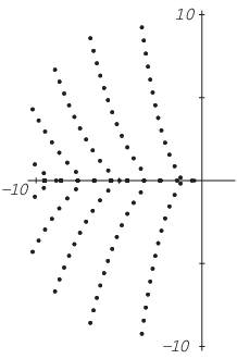
To demonstrate the sharpness of Theorem 1.1, we consider explicitly the case of scattering by a spherical obstacle in ℍn+1\mathbb{H}^{n+1}, for which X=ℍn+1−B⁡(0,r0)X=\mathbb{H}^{n+1}-B(0;r_{0}), and P=Δ0|XP=\Delta_{0}|_{X} with Dirichlet boundary conditions on ∂X\partial X. Figure 2 shows a sample resonance set for a spherical obstacle in ℍ2\mathbb{H}^{2}.

Refer to caption
Figure 2. Resonances for the spherical obstacle of radius r0=1r_{0}=1 in ℍ2\mathbb{H}^{2}. All points off the real axis have multiplicity two; on the real axis the multiplicities are more complicated.
Theorem 1.2.

If PP is the Dirichlet Laplacian on ℍn+1−B⁡(0,r0)\mathbb{H}^{n+1}-B(0;r_{0}), then

NP​(t)∼BP​tn+1.N_{P}(t)\sim B_{P}t^{n+1}.
Refer to caption
Figure 3. Resonance counting functions for spherical obstacles of radius r0r_{0} in ℍ2\mathbb{H}^{2}.

Figure 3 shows that resonance counting functions NP​(t)N_{P}(t) for spherical obstacles in ℍ2\mathbb{H}^{2} with several values of r0r_{0}. These graphs are based on exact computation of the resonances. The approximate values of the asymptotic constants for these cases are

BP≈{1.45r0=12,2.61r0=1,7.50r0=2.B_{P}\approx\begin{cases}1.45&r_{0}=\tfrac{1}{2},\\ 2.61&r_{0}=1,\\ 7.50&r_{0}=2.\end{cases}

Already at t=10t=10 we can see that the behavior of NP​(t)N_{P}(t) is consistent with the predictions of Theorem 1.2.

The paper is organized as follows. In §2 we develop basic spectral results, such as meromorphic continuation of the resolvent, in a very general “black box” perturbation setting. In §3 we narrow the context somewhat, in order to establish a nice factorization formula for the relative scattering determinant, from which the relative counting formula (1.4) follows. Another application of the factorization is the Poisson summation formula for resonances, which leads to (1.5). The process of estimating the scattering determinant begins in §4, with a formula that expresses this determinant in terms of the Poisson kernel on ℍn+1\mathbb{H}^{n+1}. In §5 we exploit this relation to prove (1.6) and complete the proof of Theorem 1.1. A few explicit spherically symmetric examples are considered in §6, which contains the proof of Theorem 1.2. Finally, the asymptotic analysis of Legendre functions that is needed for §5 and §6 is developed in the Appendix.

Acknowledgment. I would like to thank to Plamen Stefanov for suggesting the extension of his results to the hyperbolic setting. That suggestion occurred during a workshop at the Banff International Research Station, and subsequently part of the work was carried out during a stay at the Centre International des Rencontres Mathématiques in Luminy. I am grateful to both of these institutions for their support, and also thank the Emory ICIS for additional travel support for the Luminy meeting.

2. Black box perturbations

In geometric scattering theory, the term “black box” refers to a general class of perturbations of the Euclidean Laplacian in ℝn\mathbb{R}^{n} introduced by Sjöstrand-Zworski [22]. Although in standard usage this terminology is specific to the Euclidean setting, the same abstract formulation can be adapted to other settings. In this section, we will discuss black box perturbations in an asymptotically hyperbolic context. Our goal is to set up the definition of resonances by demonstrating meromorphic continuation of the resolvent, and then to prove a global estimate of the counting function. It makes sense to do this in a general setting, since only minor changes are required to adapt previously published arguments. This section essentially amounts to a review of known results.

An asymptotically hyperbolic metric on (X0,g0)(X_{0},g_{0}) admits, by definition, a compactification X¯0{\bar{X}}_{0} with boundary defining function ρ\rho such that (X¯0,ρ2​g0)({\bar{X}}_{0},\rho^{2}g_{0}) is a smooth, compact Riemannian manifold with boundary and |d​ρ|ρ2​g0=1|d\rho|_{\rho^{2}g_{0}}=1 on ∂X¯0{\partial{\bar{X}}}_{0}. We will assume that (X0,g0)(X_{0},g_{0}) is even in the sense introduced by Guillarmou [10]. This means that the Taylor series of ρ2​g0\rho^{2}g_{0} at ρ=0\rho=0 contains only even powers of ρ\rho. Under this assumption the resolvent R0​(s):=(Δg0−s⁡(n−s))−1R_{0}(s):=(\Delta_{g_{0}}-s(n-s))^{-1} admits a meromorphic to s∈ℂs\in\mathbb{C}, with poles of finite rank [10, 18].

Appropriating the terminology from the Euclidean case, we define a class of perturbations of Δg0\Delta_{g_{0}} as follows. Given a compact K0⊂X0K_{0}\subset X_{0}, we consider the Hilbert space

ℋ=ℋ0⊕L2​(X0−K0,d​g0),\mathcal{H}=\mathcal{H}_{0}\oplus L^{2}(X_{0}-K_{0},dg_{0}),

where ℋ0\mathcal{H}_{0} is some abstract Hilbert space filling in for L2​(K0,d​g0)L^{2}(K_{0},dg_{0}). On ℋ\mathcal{H} we consider a self-adjoint operator PP with domain 𝒟⊂ℋ\mathcal{D}\subset\mathcal{H}, satisfying the following assumptions:

  1. (1)

    𝒟|X0−K0⊂H2​(X0−K0,d​g0)\mathcal{D}|_{X_{0}-K_{0}}\subset H^{2}(X_{0}-K_{0},dg_{0}). If u∈H2​(X0−K0,d​g0)u\in H^{2}(X_{0}-K_{0},dg_{0}) and uu vanishes near K0K_{0}, then u∈𝒟u\in\mathcal{D}.

  2. (2)

    For u∈𝒟u\in\mathcal{D},

    (P​u)|X0−K0=Δg0​(u|X0−K0).(Pu)|_{X_{0}-K_{0}}=\Delta_{g_{0}}(u|_{X_{0}-K_{0}}).
  3. (3)

    As a map ℋ→ℋ\mathcal{H}\to\mathcal{H}, 𝟙K0​(P+i)−1\mathbbm{1}_{K_{0}}(P+i)^{-1} is compact.

Here the notations 𝟙K0:u↦u|K0\mathbbm{1}_{K_{0}}:u\mapsto u|_{K_{0}} and 𝟙X0−K0:u↦u|X0−K0\mathbbm{1}_{X_{0}-K_{0}}:u\mapsto u|_{X_{0}-K_{0}} denote the orthogonal projections ℋ→ℋ0\mathcal{H}\to\mathcal{H}_{0} and ℋ→L2​(X0−K0,d​g0)\mathcal{H}\to L^{2}(X_{0}-K_{0},dg_{0}), respectively.

We will refer to an operator PP defined as above as a black box perturbation of Δg0\Delta_{g_{0}}. Given that meromorphic continuation of the resolvent is already known for Δg0\Delta_{g_{0}}, it is relatively easy to extend this result to PP.

Theorem 2.1.

Let (X0,g0)(X_{0},g_{0}) be an even asymptotically hyperbolic manifold and PP a black box perturbation of Δg0\Delta_{g_{0}}. The resolvent RP​(s):=(P−s⁡(n−s))−1R_{P}(s):=(P-s(n-s))^{-1} admits for any NN a meromorphic continuation to Re⁡s>−N+n2\operatorname{Re}s>-N+\tfrac{n}{2} as an operator ρN​ℋ→ρ−N​ℋ\rho^{N}\mathcal{H}\to\rho^{-N}\mathcal{H}, with poles of finite rank.

Proof.

The resolvent Rg​(s)R_{g}(s) serves as a suitable parametrix for RP​(s)R_{P}(s) near the boundary. Let χ0,χ,χ1∈C0∞​(X)\chi_{0},\chi,\chi_{1}\in C^{\infty}_{0}(X) be cutoff functions equal to 1 on K0K_{0}, such that χ=0\chi=0 on the support of χ1\chi_{1} and χ0=1\chi_{0}=1 on the support of χ\chi. Let K1:=supp⁡χ1K_{1}:=\operatorname{supp}\chi_{1}, and define

P1:=P|K1,P_{1}:=P|_{K_{1}},

as an operator on ℋ|K1\mathcal{H}|_{K_{1}} with Dirichlet boundary conditions imposed on ∂K1\partial K_{1}, so that P1P_{1} is self-adjoint. We can naturally regard χ1​(P1−z)−1​χ\chi_{1}(P_{1}-z)^{-1}\chi as an operator on ℋ\mathcal{H}.

Then for z0z_{0} such that z0∉σ⁡(P)z_{0}\notin\sigma(P) we set

(2.1) M⁡(s)=χ1​(P1−z0)−1​χ+(1−χ0)​R0​(s)​(1−χ).M(s)=\chi_{1}(P_{1}-z_{0})^{-1}\chi+(1-\chi_{0})R_{0}(s)(1-\chi).

Then

(2.2) (P−s⁡(n−s))​M​(s)=I−L⁡(s),(P-s(n-s))M(s)=I-L(s),

where L⁡(s)=L1​(s0)+L2​(s,z0)+L3​(s)L(s)=L_{1}(s_{0})+L_{2}(s,z_{0})+L_{3}(s) with

L1​(z0):=−[Δg,χ1]​(P1−z0)−1​χ,L2​(s,z0):=(s⁡(n−s)−z0)​χ1​(P1−z0)−1​χ,L3​(s):=[Δg,χ0]​R0​(s)​(1−χ).\begin{split}L_{1}(z_{0})&:=-[\Delta_{g},\chi_{1}](P_{1}-z_{0})^{-1}\chi,\\ L_{2}(s,z_{0})&:=(s(n-s)-z_{0})\chi_{1}(P_{1}-z_{0})^{-1}\chi,\\ L_{3}(s)&:=[\Delta_{g},\chi_{0}]R_{0}(s)(1-\chi).\end{split}

Our goal is to prove that L⁡(s)L(s) is compact and then apply the analytic Fredholm theorem.

Consider first the error term L1​(s0)L_{1}(s_{0}), which we can write as

L1​(z0)=−[Δg,χ1]​𝟙X−K​(P1−z0)−1​χL_{1}(z_{0})=-[\Delta_{g},\chi_{1}]\mathbbm{1}_{X-K}(P_{1}-z_{0})^{-1}\chi

By definition, 𝟙X0−K0​(P1−z0)−1\mathbbm{1}_{X_{0}-K_{0}}(P_{1}-z_{0})^{-1} maps ℋ\mathcal{H} to 𝒟|X0−K0\mathcal{D}|_{X_{0}-K_{0}} and we have assumed that the latter is contained in H2​(X0−K0,d​g0)H^{2}(X_{0}-K_{0},dg_{0}). Since [Δg0,χ0][\Delta_{g_{0}},\chi_{0}] is first order with smooth coefficients whose compact support is contained in X0−K0{X_{0}-K_{0}}, we see that [Δg,χ0][\Delta_{g},\chi_{0}] is compact as a mapping H2​(X0−K0,d​g0)↦L2​(X0−K0,d​g0)H^{2}(X_{0}-K_{0},dg_{0})\mapsto L^{2}(X_{0}-K_{0},dg_{0}). Hence L1​(z0)L_{1}(z_{0}) is compact ℋ→ℋ\mathcal{H}\to\mathcal{H}.

The black box assumption that 𝟙K0​(P−i)−1\mathbbm{1}_{K_{0}}(P-i)^{-1} is compact implies that 𝟙K0​(P1−i)−1\mathbbm{1}_{K_{0}}(P_{1}-i)^{-1} is compact on ℋ|K1\mathcal{H}|_{K_{1}}. And the resolvent identity

(2.3) (P1−z)−1=(P1−i)−1​[I+(z−i)​(P1−z)−1](P_{1}-z)^{-1}=(P_{1}-i)^{-1}\Bigl[I+(z-i)(P_{1}-z)^{-1}\Bigr]

then shows that L2​(s,z0)L_{2}(s,z_{0}) is compact on ℋ\mathcal{H}. Finally, the error term L3​(s)L_{3}(s) has a smooth kernel contained in ρ∞​ρ′s​C∞​(X×X)\rho^{\infty}{\rho^{\prime}}^{s}C^{\infty}(X\times X). This implies that for N>0N>0, L3​(s)L_{3}(s) is a compact operator on ρN​ℋ\rho^{N}\mathcal{H} for Re⁡s>−N+n2\operatorname{Re}s>-N+\tfrac{n}{2}.

After adding the pieces together, these arguments show that L⁡(s)L(s) is compact on ρN​ℋ\rho^{N}\mathcal{H} for Re⁡s≥−N+n2\operatorname{Re}s\geq-N+\tfrac{n}{2}. Using the self-adjointness of P1P_{1} and the standard resolvent estimate,

(2.4) ‖(P1−z)−1‖≤1dist​(z,σ​(P))\|(P_{1}-z)^{-1}\|\leq\frac{1}{\text{dist}(z,\sigma(P))}

we can insure that ‖(P1−z0)−1‖\|(P_{1}-z_{0})^{-1}\| is small by choosing Im⁡z0\operatorname{Im}z_{0} large. Similarly, we can make ‖Rg​(s)‖\|R_{g}(s)\| small by choosing ss in the first quadrant sufficiently far from the real axis and the line Re⁡s=n2\operatorname{Re}s=\tfrac{n}{2}. Thus for some s,z0s,z_{0} we have ‖L⁡(s)‖<1\|L(s)\|<1, implying that I−L⁡(s)I-L(s) is invertible at this point. The analytic Fredholm theorem then applies to define (I−L⁡(s))−1(I-L(s))^{-1} meromorphically on ρN​ℋ\rho^{N}\mathcal{H} for Re⁡s>−N+n2\operatorname{Re}s>-N+\tfrac{n}{2}. The claimed result follows from

RP​(s)=M⁡(s)​(I−L⁡(s))−1,R_{P}(s)=M(s)(I-L(s))^{-1},

because M⁡(s)M(s) maps ρN​ℋ→ρ−N​ℋ\rho^{N}\mathcal{H}\to\rho^{-N}\mathcal{H} for Re⁡s>−N+n2\operatorname{Re}s>-N+\tfrac{n}{2}. ∎

The fact that RP​(s)R_{P}(s) admits meromorphic continuation as a bounded operator on ℋ\mathcal{H} for Re⁡s>n2\operatorname{Re}s>\tfrac{n}{2} (the N=0N=0 case) implies, as an immediate corollary, that

(2.5) σ⁡(P)∩(−∞,n24)​ is discrete.\sigma(P)\cap(-\infty,\tfrac{n^{2}}{4})\text{ is discrete}.

Theorem 2.1 allows us to define resonances associated to PP as the poles of RP​(s)R_{P}(s), with multiplicities given by

mP​(ζ):=rank⁡Resζ​RP​(s).m_{P}(\zeta):=\operatorname{rank}\operatorname{Res}_{\zeta}R_{P}(s).

Then ℛP\mathcal{R}_{P} is defined to be the set of resonances of PP, repeated according to the multiplicities mPm_{P}. The corresponding counting function is

NP​(t):=#⁡{ζ∈ℛP:|ζ−n2|≤t}.N_{P}(t):=\#\{\zeta\in\mathcal{R}_{P}:\>|\zeta-\tfrac{n}{2}|\leq t\}.

The remaining goal of this section is to establish an order-of-growth estimate for NP​(t)N_{P}(t). This requires first of all that (X0,g0)(X_{0},g_{0}) be hyperbolic near infinity, in the sense that sectional curvatures all equal −1-1 outside some compact set. (No resonance bounds are currently known in the asymptotically hyperbolic case without this extra condition.) Such asymptotically hyperbolic manifolds are even in particular.

We must also make some extra assumptions of PP:

  1. (i)

    The operator PP must be bounded below, so that the set (2.5) is actually finite.

  2. (ii)

    The singular values of the resolvent of the cutoff operator P1P_{1} introduced in the proof of Theorem 2.1 satisfy a growth estimate,

    (2.6) μk​((P1−z)−1)≤C​|Im⁡z|−12​k−1n+1,\mu_{k}((P_{1}-z)^{-1})\leq C\>|\operatorname{Im}z|^{-\frac{1}{2}}k^{-\frac{1}{n+1}},

    for some CC independent of zz and kk.

The natural way to satisfy the growth estimate (2.6) is to assume that ℋ=L2​(X,d​g)\mathcal{H}=L^{2}(X,dg) for some Riemannian manifold (X,g)(X,g), possibly with boundary, and that PP is an elliptic self-adjoint pseudodifferential operator of order 22. Then to establish (2.6) we can start by using the resolvent estimate (2.4) to estimate

μk​((P1−z)−1)≤|Im⁡z|−12​μk​(|P1−z|−12).\mu_{k}((P_{1}-z)^{-1})\leq|\operatorname{Im}z|^{-\frac{1}{2}}\>\mu_{k}(|P_{1}-z|^{-\frac{1}{2}}).

Let ΔK1\Delta_{K_{1}} denote the Dirichlet Laplacian on K1K_{1}. Since |P1−z|−12|P_{1}-z|^{-\frac{1}{2}} has order −1-1, the operator (ΔK1+1)12​|P1−z|−12(\Delta_{K_{1}}+1)^{\frac{1}{2}}|P_{1}-z|^{-\frac{1}{2}} is zeroth order and thus bounded on L2​(K1,d​g)L^{2}(K_{1},dg). Then (2.6) follows from

μk​(|P1−z|−12)≤μk​((ΔK1+1)−12)​‖(ΔK1+1)12​|P1−z|−12‖≤C​k−1n+1.\begin{split}\mu_{k}(|P_{1}-z|^{-\frac{1}{2}})&\leq\mu_{k}((\Delta_{K_{1}}+1)^{-\frac{1}{2}})\>\left\|(\Delta_{K_{1}}+1)^{\frac{1}{2}}|P_{1}-z|^{-\frac{1}{2}}\right\|\\ &\leq Ck^{-\frac{1}{n+1}}.\end{split}

(The fact that CC can be chosen independently of zz follows from the resolvent estimate (2.4).)

Theorem 2.2.

Let (X0,g0)(X_{0},g_{0}) be a conformally compact manifold, hyperbolic near infinity, and PP a black box perturbation of Δg0\Delta_{g_{0}} that satisfies the extra assumptions (i) and (ii). Then

NP​(t)=O⁡(tn+1).N_{P}(t)=O(t^{n+1}).
Proof.

This is a fairly minor generalization of the upper bound proved by Cuevas-Vodev [5] and Borthwick [1]. This is because for those arguments the interior metric enters only in the interior parametrix term, i.e., the first term on the right in (2.1). The difficult part of the upper bound analysis involves the terms supported near infinity, and this part of the argument applies immediately to PP by the assumption that P|X0−K0=Δg0P|_{X_{0}-K_{0}}=\Delta_{g_{0}}.

To apply the argument from Cuevas-Vodev, we need to check some estimates on the interior error terms L1​(z0)L_{1}(z_{0}) and L2​(s,z0)L_{2}(s,z_{0}). For the former, the fact that 𝒟|X0−K0⊂H2​(X0−K0,d​g0)\mathcal{D}|_{X_{0}-K_{0}}\subset H^{2}(X_{0}-K_{0},dg_{0}) implies that L1​(z0)L_{1}(z_{0}) is bounded as a map ℋ→H1​(K1−K0,d​g)\mathcal{H}\to H^{1}(K_{1}-K_{0},dg). If ΔK1−K0\Delta_{K_{1}-K_{0}} denotes the Dirichlet Laplacian on K1−K0K_{1}-K_{0}, then we can estimate

(2.7) μk​(L1​(z0))≤μk​((ΔK1−K0+1)−12)​‖(ΔK1−K0+1)12​L1​(s)‖≤C​k−1n+1,\begin{split}\mu_{k}(L_{1}(z_{0}))&\leq\mu_{k}\left((\Delta_{K_{1}-K_{0}}+1)^{-\frac{1}{2}}\right)\>\left\|(\Delta_{K_{1}-K_{0}}+1)^{\frac{1}{2}}L_{1}(s)\right\|\\ &\leq Ck^{-\frac{1}{n+1}},\end{split}

where we can use (2.3) and (2.4) to see that we may take CC to be independent of z0z_{0}. For the L2​(s,z0)L_{2}(s,z_{0}) term, we first of all note that (2.4) implies

‖L2​(s,z0)‖≤C​|s⁡(n−s)−z0||Im⁡z0|.\|L_{2}(s,z_{0})\|\leq C\frac{|s(n-s)-z_{0}|}{|\operatorname{Im}z_{0}|}.

By the assumption (2.6) we can immediately estimate

(2.8) μk​(L2​(s,z0))≤C​|s⁡(n−s)−z0||Im⁡z0|12​k−1n+1.\mu_{k}(L_{2}(s,z_{0}))\leq C\frac{|s(n-s)-z_{0}|}{|\operatorname{Im}z_{0}|^{\frac{1}{2}}}\>k^{-\frac{1}{n+1}}.

For the argument in [5] one needs to set z0=γ​N​(n−γ​N)z_{0}=\gamma N(n-\gamma N) for each NN such that |s|≤N|s|\leq N, so the precise dependence of these estimates on ss and z0z_{0} is significant. The estimates (2.7) and (2.8) correspond precisely to the interior estimates [5, eq.’s (2.23–4)]. The proof of [5, Prop. 1.2] then gives a bound

#{ζ∈ℛP:|ζ|≤r,arg(ζ−n2)∈[−π+ε,π−ε]}≤Cεrn+1\#\Bigl\{\zeta\in\mathcal{R}_{P}:\>|\zeta|\leq r,\>\arg(\zeta-\tfrac{n}{2})\in[-\pi+\varepsilon,\pi-\varepsilon]\Bigr\}\leq C_{\varepsilon}r^{n+1}

To fill in the missing sector containing the negative real axis, we apply the argument from Borthwick [1]. Here the interior parametrix enters only in the proof of [1, Lemma 5.2]. The required bound is that for some constant a≥na\geq n, ‖RP​(s)‖=O​(1)\|R_{P}(s)\|=O(1) for Re⁡s≥a\operatorname{Re}s\geq a. Since PP is self-adjoint and bounded below by assumption, this follows from the standard resolvent estimate. The proof of [1, Prop. 5.1] then shows that

#{ζ∈ℛP:|ζ|≤r,arg(ζ+a−n)∈[π2+ε,3​π2−ε]}≤Cεrn+1.\#\Bigl\{\zeta\in\mathcal{R}_{P}:\>|\zeta|\leq r,\>\arg(\zeta+a-n)\in[\tfrac{\pi}{2}+\varepsilon,\tfrac{3\pi}{2}-\varepsilon]\Bigr\}\leq C_{\varepsilon}r^{n+1}.

The combination of estimates in the two regions gives the global result. ∎

Remark 2.3.

Colin Guillarmou has noted a mistake in the original argument from [12], which propagated through the arguments in [5] and [1]. The faulty claim is that one can choose a family of cutoffs {χi}\{\chi^{i}\} such that ∑χi=1\sum\chi^{i}=1 in some neighborhood of ∂X¯{\partial{\bar{X}}} and also so that, in local coordinates isometric to the unit half-disk in ℍn+1\mathbb{H}^{n+1}, χi\chi^{i} factors as φ⁡(x)​ψ​(y)\varphi(x)\psi(y) in the coordinates (x,y)∈ℝn×ℝ+(x,y)\in\mathbb{R}^{n}\times\mathbb{R}_{+}. It is not possible to satisfy these assumptions simultaneously.

Fortunately, this problem is relatively easy to fix. There are two sets of cutoffs used in these proofs. (All three proofs use the same construction.) The inner cutoffs {χi}\{\chi^{i}\} must form a partition of unity near the boundary, but are not actually required to factor in local coordinates. The essential requirement for the inner cutoffs is that their derivatives satisfy quasi-analytic estimates (see [1, eq. (2.6)] for example), and this is easily obtained without reference to a factorization. The local factorization assumption is crucial only for outer cutoffs {χ1i}\{\chi_{1}^{i}\} (with χ1i=1\chi_{1}^{i}=1 on the support of χi\chi^{i}). We may keep this assumption in place because the outer cutoffs do not form a partition of unity.

3. Relative scattering theory

For this section we continue to assume, as in Theorem 2.2, a conformally compact background manifold (X0,g0)(X_{0},g_{0}) that is hyperbolic near infinity. The restriction h0=ρ2​g0|ρ=0h_{0}=\rho^{2}g_{0}|_{\rho=0} defines a Riemannian metric on ∂X¯0{\partial{\bar{X}}}_{0}, whose conformal class is independent of ρ\rho. Thus ∂X¯0{\partial{\bar{X}}}_{0} is commonly referred to as the “conformal infinity” of (X0,g0)(X_{0},g_{0}). A black box perturbation PP shares the same conformal infinity, since PP agrees with Δg0\Delta_{g_{0}} outside a compact set.

The scattering matrices SP​(s)S_{P}(s) and S0​(s)S_{0}(s), associated to PP and Δg0\Delta_{g_{0}}, respectively, are pseudodifferential operators on ∂X¯0{\partial{\bar{X}}}_{0} defined as in [16, 8]. Away from the diagonal, we can realize the kernel of the scattering matrix as a boundary limit of the resolvent:

(3.1) S∗​(s,x,x′)=limρ,ρ′→0(ρ​ρ′)−s​R∗​(s,z,z′)for ​x≠x′.S_{*}(s;x,x^{\prime})=\lim_{\rho,\rho^{\prime}\to 0}(\rho\rho^{\prime})^{-s}R_{*}(s;z,z^{\prime})\qquad\text{for }x\neq x^{\prime}.

where ∗* = PP or 00. (This relationship can be extended to the diagonal if one is sufficiently careful - see [16].) This connection allows us to see that SP​(s)S_{P}(s) and S0​(s)S_{0}(s) differ by a smoothing operator, as follows. By applying RP​(s)R_{P}(s) to (2.2) from the left, we obtain the identity

RP​(s)=M⁡(s)+RP​(s)​L​(s).R_{P}(s)=M(s)+R_{P}(s)L(s).

Then taking boundary limits as in (3.1) gives the kernel of SP​(s)S_{P}(s) on the left, while on the right we obtain the kernel of S0​(s)S_{0}(s) as the limit of M⁡(s)M(s), plus a smooth contribution from the L⁡(s)L(s) term. This implies that the relative scattering matrix SP​(s)​S0​(s)−1S_{P}(s)S_{0}(s)^{-1} is determinant class, and we define the relative scattering determinant

(3.2) τ⁡(s):=detSP​(s)​S0​(s)−1.\tau(s):=\det S_{P}(s)S_{0}(s)^{-1}.

Let H∗​(s)H_{*}(s) denote the Hadamard product over the resonance set ℛ∗\mathcal{R}_{*}:

(3.3) H∗​(s):=∏ζ∈ℛ∗E⁡(sζ,n+1),H_{*}(s):=\prod_{\zeta\in\mathcal{R}_{*}}E\Bigl(\frac{s}{\zeta},n+1\Bigr),

where

E⁡(z,p):=(1−z)​exp⁡(z+z2z+⋯+zpp).E(z,p):=(1-z)\exp\Bigl(z+\frac{z^{2}}{z}+\dots+\frac{z^{p}}{p}\Bigr).
Proposition 3.1.

Assume that (X0,g0)(X_{0},g_{0}) is conformally compact and hyperbolic near infinity, and PP is a black box perturbation of Δg0\Delta_{g_{0}} satisfying the extra assumptions (i) and (ii) from §2. The relative scattering determinant admits a factorization

(3.4) τ⁡(s)=eq⁡(s)​HP​(n−s)HP​(s)​H0​(s)H0​(n−s),\tau(s)=e^{q(s)}\frac{H_{P}(n-s)}{H_{P}(s)}\frac{H_{0}(s)}{H_{0}(n-s)},

where q⁡(s)q(s) is a polynomial of degree at most n+1n+1.

Proof.

Since structure near infinity is unchanged from (X0,g0)(X_{0},g_{0}), the arguments of Guillarmou [11] relating the resolvent and scattering pole multiplicities apply to PP. Thus the proof of [1, Prop. 7.2] shows that (3.4) holds with with q⁡(s)q(s) a polynomial of unknown degree.

To control the degree, we use the fact that PP is bounded from below to obtain

‖RP​(s)‖=O⁡(1), for ​Re⁡s≥a,\|R_{P}(s)\|=O(1),\text{ for }\operatorname{Re}s\geq a,

for some a≥na\geq n. Then the proof of [1, Lemma 5.2] gives that

|ϑP​(s)|<eCη​⟨s⟩n+1,|\vartheta_{P}(s)|<e^{C_{\eta}\langle s\rangle^{n+1}},

for Re⁡s<a−n\operatorname{Re}s<a-n with dist(s,−ℕ0)>η(s,-\mathbb{N}_{0})>\eta. The same estimate applies to ϑ0​(s)\vartheta_{0}(s). In the formula

ϑP​(s)=e−q⁡(s)​H0​(n−s)H0​(s)​HP​(s)HP​(n−s)​ϑ0​(s),\vartheta_{P}(s)=e^{-q(s)}\frac{H_{0}(n-s)}{H_{0}(s)}\frac{H_{P}(s)}{H_{P}(n-s)}\>\vartheta_{0}(s),

the Hadamard products have order n+1n+1. Thus the ϑ∗​(s)\vartheta_{*}(s) estimates imply that |q⁡(s)|≤C​|s|n+1+δ|q(s)|\leq C|s|^{n+1+\delta} in the half-plane Re⁡s<a−n\operatorname{Re}s<a-n, for any δ>0\delta>0. Since q⁡(s)q(s) is already known to be polynomial, the degree of q⁡(s)q(s) is at most n+1n+1. ∎

One nice application of Proposition 3.1 is a Jensen-type formula connecting the resonance counting functions to a contour integral involving the relative scattering determinant. To state this we introduce the relative scattering phase of PP, defined as

σ⁡(ξ):=i2​π​log⁡τ⁡(12+i​ξ),\sigma(\xi):=\frac{i}{2\pi}\log\tau(\tfrac{1}{2}+i\xi),

with branches of the log chosen so that σ⁡(ξ)\sigma(\xi) is continuous starting from σ⁡(0)=0\sigma(0)=0. By the properties of the relative scattering matrix, σ⁡(ξ)\sigma(\xi) is real and σ⁡(−ξ)=−σ⁡(ξ)\sigma(-\xi)=-\sigma(\xi).

The following relative counting formula is the asymptotically hyperbolic analog of a formula developed by Froese [7] for Schrödinger operators in the Euclidean setting.

Proposition 3.2.

Assume that PP is a black box perturbation of (X0,g0)(X_{0},g_{0}) as in Proposition 3.1. As a→∞a\to\infty,

∫0aNP​(t)−N0​(t)t​𝑑t=2​∫0aσ⁡(t)t​𝑑t+12​π​∫−π2π2log|τ⁡(n2+a​ei​θ)|𝑑θ+O⁡(log⁡a).\int_{0}^{a}\frac{N_{P}(t)-N_{0}(t)}{t}\>dt=2\int_{0}^{a}\frac{\sigma(t)}{t}\>dt+\frac{1}{2\pi}\int_{-\frac{\pi}{2}}^{\frac{\pi}{2}}\log|\tau(\tfrac{n}{2}+ae^{i\theta})|\>d\theta+O(\log a).
Proof.

According to Proposition 3.1, for Re⁡(s)>n2\operatorname{Re}(s)>\tfrac{n}{2}, τ⁡(s)\tau(s) has zeros when n−s∈ℛPn-s\in\mathcal{R}_{P} or s∈ℛ0s\in\mathcal{R}_{0} and the latter case occurs only if s⁡(n−s)s(n-s) lies in the discrete spectrum of Δg0\Delta_{g_{0}}. Likewise, poles of τ⁡(s)\tau(s) for Re⁡s>n2\operatorname{Re}s>\tfrac{n}{2} occur when either n−s∈ℛ0n-s\in\mathcal{R}_{0} or s∈ℛPs\in\mathcal{R}_{P}, the latter only if s⁡(n−s)s(n-s) lies in the discrete spectrum of PP. All of these are counted with multiplicity of course.

Let η\eta denote the contour (n2+texp(i[−π/2,π/2]))∪[n2+it,n2−it](\tfrac{n}{2}+t\exp(i[-\pi/2,\pi/2]))\cup[\tfrac{n}{2}+it,\tfrac{n}{2}-it], as shown in Figure 4. Assuming tt is not the absolute value of a resonance in ℛ\mathcal{R} or ℛ0\mathcal{R}_{0}, we have

12​π​i​∮ητ′τ​(s)​𝑑s=NP​(t)−N0​(t)−2​dP​(t)+2​d0​(t),\frac{1}{2\pi i}\oint_{\eta}\frac{\tau^{\prime}}{\tau}(s)\>ds=N_{P}(t)-N_{0}(t)-2d_{P}(t)+2d_{0}(t),

where d∗​(u)d_{*}(u) is the counting function for the (finite) set ℛ∗∩(n2,∞)\mathcal{R}_{*}\cap(\tfrac{n}{2},\infty) (the resonances coming from the discrete spectrum).

Refer to caption
Figure 4. The contour η\eta.

Evaluating the contour integral yields

12​π​i​∮ητ′τ​(s)​𝑑s=Im⁡12​π​∮ητ′τ​(s)​𝑑s=∫−ttσ′​(ξ)​𝑑ξ+Im⁡12​π​∫−π2π2τ′τ​(n2+t​ei​θ)​i​t​ei​θ​𝑑θ=2​σ​(t)+12​π​∫−π2π2t​∂∂t​log⁡|τ⁡(n2+t​ei​θ)|​dθ.\begin{split}\frac{1}{2\pi i}\oint_{\eta}\frac{\tau^{\prime}}{\tau}(s)\>ds&=\operatorname{Im}\frac{1}{2\pi}\oint_{\eta}\frac{\tau^{\prime}}{\tau}(s)\>ds\\ &=\int_{-t}^{t}\sigma^{\prime}(\xi)\>d\xi+\operatorname{Im}\frac{1}{2\pi}\int_{-\frac{\pi}{2}}^{\frac{\pi}{2}}\frac{\tau^{\prime}}{\tau}(\tfrac{n}{2}+te^{i\theta})\>ite^{i\theta}\>d\theta\\ &=2\sigma(t)+\frac{1}{2\pi}\int_{-\frac{\pi}{2}}^{\frac{\pi}{2}}t\frac{\partial}{\partial t}\log|\tau(\tfrac{n}{2}+te^{i\theta})|\>d\theta.\end{split}

Now if we divide by tt and integrate, we obtain the claimed formula with remainder given by

2​∫0adP​(t)−d0​(t)t​𝑑t=O⁡(log⁡a).2\int_{0}^{a}\frac{d_{P}(t)-d_{0}(t)}{t}\>dt=O(\log a).

∎

Our second important application of Proposition 3.1 is to establish the Poisson formula, which will lead to Weyl-type asymptotics for the relative scattering phase. Define the meromorphic function Υ∗​(s)\Upsilon_{*}(s) by

(2​s−n)​0−tr⁡[R∗​(s)−R∗​(1−s)],(2s-n)\operatorname{0-tr}[R_{*}(s)-R_{*}(1-s)],

for s∉ℤ/2s\notin\mathbb{Z}/2. The connection between Υ∗​(s)\Upsilon_{*}(s) and the relative scattering determinant established by Patterson-Perry [20, Prop. 5.3 and Lemma 6.7] depends only on the structure of model neighborhoods near infinity, and so carries over to our case without alteration. This yields the following Birman-Krein type formula:

Proposition 3.3.

For s∉ℤ/2s\notin\mathbb{Z}/2 we have the meromorphic identity,

−∂slogτ(s)=ΥP(s)−Υ0(s).-\partial_{s}\log\tau(s)=\Upsilon_{P}(s)-\Upsilon_{0}(s).

By the functional calculus, Υ∗​(n2+i​ξ)\Upsilon_{*}(\tfrac{n}{2}+i\xi) is essentially the Fourier transform of the continuous part of the wave 0-trace (see [1, Lemma 8.1] for the precise statement). By Propositions 3.1 and 3.3 we can write

ΥP​(s)−Υ0​(s)=∂slog⁡[eq⁡(s)​HP​(s)HP​(n−s)​H0​(n−s)H0​(s)]\Upsilon_{P}(s)-\Upsilon_{0}(s)=\partial_{s}\log\left[e^{q(s)}\frac{H_{P}(s)}{H_{P}(n-s)}\frac{H_{0}(n-s)}{H_{0}(s)}\right]

Taking the Fourier transform just as in the proof of [1, Thm. 1.2] then gives a relative Poisson formula:

Theorem 3.4.

Assume that PP is a black box perturbation of (X0,g0)(X_{0},g_{0}) as in Proposition 3.1. The difference of regularized wave traces satisfies

0−tr⁡[cos⁡(t​P−n24)]−0−tr⁡[cos⁡(t​Δg0−n24)]=12​∑ζ∈ℛPe(ζ−n2)​|t|−12​∑ζ∈ℛ0e(ζ−n2)​|t|,\begin{split}&\operatorname{0-tr}\left[\cos\left(t\sqrt{P-\tfrac{n^{2}}{4}}\,\right)\right]-\operatorname{0-tr}\left[\cos\left(t\sqrt{\Delta_{g_{0}}-\tfrac{n^{2}}{4}}\,\right)\right]\\ &\qquad=\frac{1}{2}\sum_{\zeta\in\mathcal{R}_{P}}e^{(\zeta-\frac{n}{2})|t|}-\frac{1}{2}\sum_{\zeta\in\mathcal{R}_{0}}e^{(\zeta-\frac{n}{2})|t|},\end{split}

in the sense of distributions on ℝ−{0}\mathbb{R}-\{0\}.

The desired asymptotics of the scattering phase correspond to the big singularity of the wave trace at t=0t=0. This singularity is very much analogous to that worked out by Duistermaat-Guillemin [6] in the compact case. The following result was proven for Riemann surfaces, possible with internal boundary, by Guillopé-Zworski [14, Lemma 6.2] and for higher dimensional asymptotically hyperbolic manifolds (without boundary) by Joshi-Sá Baretto [17].

Let (X0,g0)(X_{0},g_{0}) be a Riemannian manifold that is conformally compact and hyperbolic outside some compact set K0⊂X0K_{0}\subset X_{0} (a more restrictive class than asymptotically hyperbolic). Then we consider another Riemannian manifold (X,g)(X,g), possibly with boundary, with compact K⊂XK\subset X such that (X−K,g)≅(X0−K0,g0)(X-K,g)\cong(X_{0}-K_{0},g_{0}). Let Δg\Delta_{g} denote the Laplacian on (X,g)(X,g). We may also include a potential V∈C0∞​(X)V\in C^{\infty}_{0}(X), supported in KK. Given this setup we define the operator

P:=Δg+V,P:=\Delta_{g}+V,

acting on L2​(X,d​g)L^{2}(X,dg) with some self-adjoint boundary condition imposed on the internal boundary ∂X\partial X. Clearly PP is a black box perturbation of Δg0\Delta_{g_{0}}, and it satisfies assumptions (i) and (ii) of §2 by the remark preceding Theorem 2.2.

Proposition 3.5.

Assume that P=Δg+VP=\Delta_{g}+V as described above. If ψ∈C0∞​(ℝ)\psi\in C^{\infty}_{0}(\mathbb{R}) has support in a sufficiently small neighborhood of 00 and ψ=1\psi=1 in some smaller neighborhood of 00, then

(3.5) ∫−∞∞e−i​t​ξ​ψ​(t)​0−tr⁡[cos⁡(t​P−n2/4)]​𝑑t∼∑k=0∞ak​|ξ|n−2​k,\int_{-\infty}^{\infty}e^{-it\xi}\psi(t)\operatorname{0-tr}\left[\cos\left(t\sqrt{\smash[b]{P-n^{2}/4}}\,\right)\right]\>dt\sim\sum_{k=0}^{\infty}a_{k}|\xi|^{n-2k},

where

a0=2−n​π−n−12Γ⁡(n+12)​0−vol⁡(X,g).a_{0}=\frac{2^{-n}\pi^{-\frac{n-1}{2}}}{\Gamma(\frac{n+1}{2})}\operatorname{0-vol}(X,g).
Proof.

By finite speed of propagation we can use cutoffs to split the wave trace into internal and external pieces:

0−tr⁡[cos⁡(t​P−n2/4)]=tr⁡[cos⁡(t​P1−n2/4)​χ]+0−tr⁡[cos⁡(t​Δg0−n2/4)​(1−χ)].\begin{split}\operatorname{0-tr}\left[\cos\left(t\sqrt{\smash[b]{P-n^{2}/4}}\,\right)\right]&=\operatorname{tr}\left[\cos\left(t\sqrt{\smash[b]{P_{1}-n^{2}/4}}\,\right)\chi\right]\\ &\qquad+\operatorname{0-tr}\left[\cos\left(t\sqrt{\smash[b]{\Delta_{g_{0}}-n^{2}/4}}\,\right)(1-\chi)\right].\end{split}

The small time behavior of the first term (which is an actual trace) is given by Ivrii’s result for compact manifolds with boundary [15]. For the exterior term we can apply [17]. ∎

Using Proposition 3.3 and the Fourier transform relationship between Υ∗​(ξ)\Upsilon_{*}(\xi) and the wave 00-trace, we can extract from Proposition 3.5 the asymptotic behavior of the relative scattering phase, defined as

σ⁡(ξ):=i2​π​log⁡τ⁡(12+i​ξ),\sigma(\xi):=\frac{i}{2\pi}\log\tau(\tfrac{1}{2}+i\xi),

with branches of the log chosen so that σ⁡(ξ)\sigma(\xi) is continuous starting from σ⁡(0)=0\sigma(0)=0. By the properties of the relative scattering matrix, σ⁡(ξ)\sigma(\xi) is real and σ⁡(−ξ)=−σ⁡(ξ)\sigma(-\xi)=-\sigma(\xi).

Corollary 3.6.

As ξ→+∞\xi\to+\infty,

σ⁡(ξ)=(4​π)−n+12Γ⁡(n+32)​[vol⁡(K,g)−vol⁡(K0,g0)]​ξn+1+O⁡(ξn).\sigma(\xi)=\frac{(4\pi)^{-\frac{n+1}{2}}}{\Gamma(\frac{n+3}{2})}\bigl[\operatorname{vol}(K,g)-\operatorname{vol}(K_{0},g_{0})\bigr]\>\xi^{n+1}+O(\xi^{n}).

The argument to derive Corollary 3.6 from Theorem 3.4 and Proposition 3.5 requires almost no change from that given for n=1n=1 by Guillopé-Zworski [14, Thm. 1.5], so we omit the details. Proposition 3.1 (and in particular the bound on the order of τ⁡(s)\tau(s)) supplies the additional information needed to extend their result to n>1n>1. The leading coefficient is initially given by a difference of 00-volumes, and we use (X−K,g)≅(X0−K0,g0)(X-K,g)\cong(X_{0}-K_{0},g_{0}) to reduce this to a difference of the volumes of KK and K0K_{0}.

4. Poisson kernel formulas

Since the asymptotics of σ⁡(t)\sigma(t) are given by Corollary 3.6, application of the formula from Proposition 3.2 requires only estimation of |τ⁡(s)||\tau(s)| in the half-plane Re⁡s>n2\operatorname{Re}s>\tfrac{n}{2}. To facilitate this estimation, we need a more explicit realization of τ⁡(s)\tau(s) as a Fredholm determinant. This realization will involve the Poisson kernel for the background metric (X0,g0)(X_{0},g_{0}). For the moment we assume only that (X0,g0)(X_{0},g_{0}) is an even asymptotically hyperbolic metric.

The Poisson kernel can be derived from the kernel of the resolvent R0​(s)R_{0}(s) by the limit

E0​(s,z,x′):=limρ′→0ρ′−s​R0​(s,z,z′),E_{0}(s;z,x^{\prime}):=\lim_{\rho^{\prime}\to 0}{\rho^{\prime}}^{-s}R_{0}(s;z,z^{\prime}),

for z∈X0z\in X_{0} and x′∈∂X¯0x^{\prime}\in{\partial{\bar{X}}}_{0}. This kernel defines the Poisson operator

E0​(s):L2​(∂X¯0,d​h)→ρ−N​L2​(X0,d​g0),E_{0}(s):L^{2}({\partial{\bar{X}}}_{0},dh)\to\rho^{-N}L^{2}(X_{0},dg_{0}),

for Re⁡s>−N+n2\operatorname{Re}s>-N+\tfrac{n}{2}, where hh is the metric induced on ∂X¯0{\partial{\bar{X}}}_{0} by ρ2​g0\rho^{2}g_{0}. For f∈C∞​(∂X¯)f\in C^{\infty}({\partial{\bar{X}}}) we can solve (Δg0−s⁡(n−s))​u=0(\Delta_{g_{0}}-s(n-s))u=0 by setting u=E0​(s)​fu=E_{0}(s)f. Moreover, for Re⁡s≥n2\operatorname{Re}s\geq\tfrac{n}{2} with s⁡(n−s)s(n-s) not in the discrete spectrum of Δg0\Delta_{g_{0}}, uu has a two-part asymptotic expansion as ρ→0\rho\to 0,

(4.1) (2​s−n)​E0​(s)​f∼ρn−s​f+ρs​S0​(s)​f,(2s-n)E_{0}(s)f\sim\rho^{n-s}f+\rho^{s}S_{0}(s)f,

where S0​(s)S_{0}(s) is the scattering matrix. This expansion, for general choice of ff, uniquely determines the scattering matrix via meromorphic continuation.

The same construction works for SP​(s)S_{P}(s). In particular, if we manage to find a family of solutions of (P−s⁡(n−s))​u=0(P-s(n-s))u=0 such that

(2​s−n)​u∼ρn−s​f+ρs​f′,(2s-n)u\sim\rho^{n-s}f+\rho^{s}f^{\prime},

for f∈C∞​(∂X¯0)f\in C^{\infty}({\partial{\bar{X}}}_{0}) and ss in some suitable region, then SP​(s)S_{P}(s) can be identified as the map f↦f′f\mapsto f^{\prime}.

Lemma 4.1.

Suppose that PP is a black box perturbation of (X0,g0)(X_{0},g_{0}) with support in K0K_{0}. Let χ1,χ2∈C0∞​(X)\chi_{1},\chi_{2}\in C^{\infty}_{0}(X) be cutoff functions such that K0⊂{χ1=1}K_{0}\subset\{\chi_{1}=1\} and suppχ1⊂{χ2=1}\operatorname{supp}\chi_{1}\subset\{\chi_{2}=1\}. The relative scattering matrix can be written as the Fredholm determinant

τ⁡(s)=det(1+Q⁡(s)),\tau(s)=\det(1+Q(s)),

where

Q⁡(s):=(2​s−n)​E0​(s)t​[Δ0,χ2]​RP​(s)​[Δ0,χ1]​E0​(n−s).Q(s):=(2s-n)E_{0}(s)^{t}[\Delta_{0},\chi_{2}]R_{P}(s)[\Delta_{0},\chi_{1}]E_{0}(n-s).
Proof.

Since all of the operators in question are meromorphic families, we can restrict ss to some convenient set like Re⁡s=n2\operatorname{Re}s=\tfrac{n}{2}, s≠n2s\neq\tfrac{n}{2} to avoid poles in the proof.

Given f∈C∞​(∂X¯0)f\in C^{\infty}({\partial{\bar{X}}}_{0}), consider the ansatz

(4.2) u=(1−χ1)​E0​(s)​f+u′,u=(1-\chi_{1})E_{0}(s)f+u^{\prime},

as a solution of (P−s⁡(n−s))​u=0(P-s(n-s))u=0. Then P⁡(1−χ1)=Δ0​(1−χ1)P(1-\chi_{1})=\Delta_{0}(1-\chi_{1}) implies that

−[Δ0,χ1]​E0​(s)​f+(P−s⁡(n−s))​u′=0.-[\Delta_{0},\chi_{1}]E_{0}(s)f+(P-s(n-s))u^{\prime}=0.

After applying RP​(s)R_{P}(s) on the left, we see that (P−s⁡(n−s))​u=0(P-s(n-s))u=0 may be solved by setting

u′=RP​(s)​[Δ0,χ1]​E0​(s)​f.u^{\prime}=R_{P}(s)[\Delta_{0},\chi_{1}]E_{0}(s)f.

Using the assumption on supports of χ1\chi_{1} and χ2\chi_{2}, we can derive

(Δ0−s⁡(n−s))​(1−χ2)​u′=−[Δ0,χ2]​u′+(1−χ2)​(P−s⁡(n−s))​u′=−[Δ0,χ2]​u′.\begin{split}(\Delta_{0}-s(n-s))(1-\chi_{2})u^{\prime}&=-[\Delta_{0},\chi_{2}]u^{\prime}+(1-\chi_{2})(P-s(n-s))u^{\prime}\\ &=-[\Delta_{0},\chi_{2}]u^{\prime}.\end{split}

This is compactly supported, so that R0​(s)R_{0}(s) may be applied to give

(1−χ2)​u′=−R0​(s)​[Δ0,χ2]​u′=−R0​(s)​[Δ0,χ2]​RP​(s)​[Δ0,χ1]​E0​(s)​f.\begin{split}(1-\chi_{2})u^{\prime}&=-R_{0}(s)[\Delta_{0},\chi_{2}]u^{\prime}\\ &=-R_{0}(s)[\Delta_{0},\chi_{2}]R_{P}(s)[\Delta_{0},\chi_{1}]E_{0}(s)f.\end{split}

From this we can deduce the asymptotic behavior of u′u^{\prime} as ρ→0\rho\to 0,

u′∼−ρs​E0​(s)t​[Δ0,χ2]​RP​(s)​[Δ0,χ1]​E0​(s)​f.u^{\prime}\sim-\rho^{s}E_{0}(s)^{t}[\Delta_{0},\chi_{2}]R_{P}(s)[\Delta_{0},\chi_{1}]E_{0}(s)f.

Using the definition (4.2) of uu and the known asymptotic (4.1) for E0​(s)​fE_{0}(s)f, we thus derive the expansion

(2​s−n)​u∼ρn−s​f+ρs​S0​(s)​f−ρs​(2​s−n)​E0​(s)t​[Δ0,χ2]​RP​(s)​[Δ0,χ1]​E0​(s)​f.(2s-n)u\sim\rho^{n-s}f+\rho^{s}S_{0}(s)f-\rho^{s}(2s-n)E_{0}(s)^{t}[\Delta_{0},\chi_{2}]R_{P}(s)[\Delta_{0},\chi_{1}]E_{0}(s)f.

We can rewrite this as

(4.3) (2​s−n)​u∼ρn−s​f+(1+Q⁡(s))​S0​(s)​f,(2s-n)u\sim\rho^{n-s}f+(1+Q(s))S_{0}(s)f,

using the identity

E0​(s)=−E0​(n−s)​S0​(s),E_{0}(s)=-E_{0}(n-s)S_{0}(s),

which follows immediately from (4.1). From (4.3) we read off that

SP​(s)=(1+Q⁡(s))​S0​(s),S_{P}(s)=(1+Q(s))S_{0}(s),

and the determinant follows. ∎

In order to use Lemma 4.1 to estimate τ⁡(s)\tau(s), we need explicit knowledge of the background Poisson operator E0​(s)E_{0}(s). At this point we specialize to (X0,g0)≅ℍn+1(X_{0},g_{0})\cong\mathbb{H}^{n+1} and work out formulas for E0​(s,z,x′)E_{0}(s;z,x^{\prime}). In the usual ℍn\mathbb{H}^{n} coordinates, z=(x,y)∈ℝn×ℝ+z=(x,y)\in\mathbb{R}^{n}\times\mathbb{R}_{+}, we can read off immediately from (1.1) that

E0​(s,z,x′)=2−2​s−1​π−n2​Γ⁡(s)Γ⁡(s−n2+1)​[yy2+|x−x′|2]s.E_{0}(s;z,x^{\prime})=2^{-2s-1}\pi^{-\tfrac{n}{2}}\frac{\Gamma(s)}{\Gamma(s-\tfrac{n}{2}+1)}\biggl[\frac{y}{y^{2}+|x-x^{\prime}|^{2}}\biggr]^{s}.

However, our application requires that E0​(s,⋅,⋅)E_{0}(s;\cdot,\cdot) be written in geodesic polar coordinates and then decomposed into spherical harmonics. The easiest way to do this is to rederive E0​(s,⋅,⋅)E_{0}(s;\cdot,\cdot) from scratch.

In geodesic polar coordinates, ℍn+1≅ℝ+×Sn\mathbb{H}^{n+1}\cong\mathbb{R}_{+}\times S^{n} and the hyperbolic metric is given by

g0=d​r2+sinh2⁡r​d​ω2,g_{0}=dr^{2}+\sinh^{2}r\>d\omega^{2},

where d​ω2d\omega^{2} denotes the standard sphere metric on SnS^{n}. It is thus natural to adopt the boundary defining function

(4.4) ρ=2​e−r,\rho=2e^{-r},

so that hh, the metric induced on ∂X¯0{\partial{\bar{X}}}_{0} by ρ2​g0\rho^{2}g_{0}, is also the standard sphere metric.

The Laplacian on ℍn+1\mathbb{H}^{n+1} is

Δ0=−1sinhn⁡r∂r(sinhnr∂r)+1sinh2⁡rΔSn.\Delta_{0}=-\frac{1}{\sinh^{n}r}\partial_{r}(\sinh^{n}r\>\partial_{r})+\frac{1}{\sinh^{2}r}\Delta_{S^{n}}.

The eigenfunctions of ΔSn\Delta_{S^{n}} are spherical harmonics YlmY_{l}^{m} with

ΔSn​Ylm=l⁡(l+n−1)​Ylm.\Delta_{S^{n}}Y_{l}^{m}=l(l+n-1)Y_{l}^{m}.

Here l=0,1,2,…l=0,1,2,\dots and m=0,1,…,hn​(l)m=0,1,\dots,h_{n}(l) with

(4.5) hn​(l):=2​l+n−1n−1​(l+n−2n−2).h_{n}(l):=\frac{2l+n-1}{n-1}\binom{l+n-2}{n-2}.
Proposition 4.2.

For ℍn+1\mathbb{H}^{n+1} the Poisson kernel in geodesic polar coordinates admits an expansion

(4.6) E0​(s,r,ω,ω′)=∑l=0∞∑m=1hn​(l)al​(s,r)​Ylm​(ω)​Ylm​(ω′)¯,E_{0}(s;r,\omega,\omega^{\prime})=\sum_{l=0}^{\infty}\sum_{m=1}^{h_{n}(l)}a_{l}(s;r)Y_{l}^{m}(\omega)\overline{Y_{l}^{m}(\omega^{\prime})},

with coefficients given by

al​(s,r)=2n−12−s​π1/2​Γ⁡(l+s)Γ⁡(s−n2+1)​(sinh⁡r)−n−12​Ps−n+12−l−n−12​(cosh⁡r),a_{l}(s;r)=2^{\frac{n-1}{2}-s}\pi^{1/2}\frac{\Gamma(l+s)}{\Gamma(s-\tfrac{n}{2}+1)}(\sinh r)^{-\frac{n-1}{2}}P_{s-\frac{n+1}{2}}^{-l-\frac{n-1}{2}}(\cosh r),

where Pνμ​(z)P_{\nu}^{\mu}(z) is the Legendre function.

Proof.

If we expand the Poisson kernel with respect to the spherical harmonic basis as in (4.6), then the equation (Δg−s⁡(n−s))​E0​(s)=0(\Delta_{g}-s(n-s))E_{0}(s)=0 implies the coefficient equations,

(4.7) −∂r2al−ncothr∂ral+(l⁡(l+n−1)sinh2⁡r−s(n−s))al=0.-\partial_{r}^{2}a_{l}-n\coth r\>\partial_{r}a_{l}+\left(\frac{l(l+n-1)}{\sinh^{2}r}-s(n-s)\right)a_{l}=0.

After a standard change of variables this becomes the Legendre equation. Since the Poisson kernel is smooth in the interior, we select the Legendre solutions that are recessive for r→0r\to 0, namely

al​(s,r)=Al​(s)​(sinh⁡r)−n−12​Ps−n+12−l−n−12​(cosh⁡r),a_{l}(s;r)=A_{l}(s)(\sinh r)^{-\frac{n-1}{2}}P_{s-\frac{n+1}{2}}^{-l-\frac{n-1}{2}}(\cosh r),

for some constants Al​(s)A_{l}(s).

The constant Al​(s)A_{l}(s) may be identified from the asymptotic expansion (4.1) as r→∞r\to\infty. For the coefficients this expansion implies that

(2​s−n)​al​(s,r)∼ρn−s+[S0​(s)]l​ρs,(2s-n)a_{l}(s;r)\sim\rho^{n-s}+[S_{0}(s)]_{l}\rho^{s},

with [S0​(s)]l​(s)[S_{0}(s)]_{l}(s) the matrix elements of the scattering matrix S0​(s)S_{0}(s), which will be diagonal in the spherical harmonic basis.

Using (4.4) and the well-known asymptotics of the Legendre PP-function, the leading terms in our ansatz as r→∞r\to\infty are

(sinh⁡r)−n−12​Ps−n+12−l−n−12​(cosh⁡r)∼2s−n+12π−1/2Γ⁡(s−n2)Γ⁡(l+s)ρn−s+2−s+n−12π−1/2Γ⁡(n2−s)Γ⁡(l+n−s)ρs,\begin{split}(\sinh r)^{-\frac{n-1}{2}}P_{s-\frac{n+1}{2}}^{-l-\frac{n-1}{2}}(\cosh r)&\sim 2^{s-\frac{n+1}{2}}\pi^{-1/2}\frac{\Gamma(s-\tfrac{n}{2})}{\Gamma(l+s)}\rho^{n-s}\\ &\qquad+2^{-s+\frac{n-1}{2}}\pi^{-1/2}\frac{\Gamma(\tfrac{n}{2}-s)}{\Gamma(l+n-s)}\rho^{s},\end{split}

from which we deduce

Al​(s)=2n−12−s​π1/2​Γ⁡(l+s)Γ⁡(s−n2+1).A_{l}(s)=2^{\frac{n-1}{2}-s}\pi^{1/2}\frac{\Gamma(l+s)}{\Gamma(s-\tfrac{n}{2}+1)}.

∎

For future reference, note that we can also read off from this construction the (well-known) matrix elements of S0​(s)S_{0}(s),

(4.8) [S0​(s)]l=2n−2​s​Γ⁡(n2−s)Γ⁡(s−n2)​Γ⁡(l+s)Γ⁡(l+n−s).[S_{0}(s)]_{l}=2^{n-2s}\frac{\Gamma(\tfrac{n}{2}-s)}{\Gamma(s-\tfrac{n}{2})}\frac{\Gamma(l+s)}{\Gamma(l+n-s)}.

5. Scattering determinant estimates

In this section we will combine the formula for τ⁡(s)\tau(s) from Lemma 4.1 with the explicit Fourier coefficients of the Poisson kernel given in Proposition 4.2. We can then use estimates of the Legendre PP-function developed in the Appendix to produce an estimate for the |τ⁡(s)||\tau(s)| term in the counting formula from Proposition 3.2.

Throughout this section, the background metric is restricted to (X0,g0)≅ℍn+1(X_{0},g_{0})\cong\mathbb{H}^{n+1}. We assume that PP is a black box perturbation of the hyperbolic Laplacian Δ0\Delta_{0}. As in §1, the support of the perturbation is assumed to lie within

K0:={r≤r0}.K_{0}:=\{r\leq r_{0}\}.

The main result of this section is the following:

Theorem 5.1.

Let PP be a black box perturbation of the hyperbolic Laplacian Δ0\Delta_{0} on ℍn+1\mathbb{H}^{n+1}. For a∈n2+ℕa\in\tfrac{n}{2}+\mathbb{N}, we can estimate

12​π​∫−π2π2log⁡|τ⁡(n2+a​ei​θ)|​𝑑θ≤BP(2)​an+1+o⁡(an+1),\frac{1}{2\pi}\int_{-\frac{\pi}{2}}^{\frac{\pi}{2}}\log|\tau(\tfrac{n}{2}+ae^{i\theta})|\>d\theta\leq B_{P}^{(2)}a^{n+1}+o(a^{n+1}),

as a→∞a\to\infty, where BP(2)B_{P}^{(2)} was defined by (1.7).

Before proceeding with the proof, we note that the combination of Proposition 3.2, Corollary 3.6, and Theorem 5.1, immediately yields the proof of Theorem 1.1. Note also that the restriction to P=Δg+VP=\Delta_{g}+V (from the more general black box class) is needed only for Corollary 3.6.

The proof of Theorem 5.1 will be broken into several stages, starting with:

Lemma 5.2.

Assuming PP and r0r_{0} are defined as above, fix some small ε>0\varepsilon>0 and η>0\eta>0 and define rj:=r0+j​ηr_{j}:=r_{0}+j\eta. For Re⁡s≥n2\operatorname{Re}s\geq\tfrac{n}{2} with dist(s⁡(n−s),σ⁡(P))≥ε(s(n-s),\sigma(P))\geq\varepsilon, the relative scattering determinant can be estimated by

(5.1) log⁡|τ⁡(s)|≤∑l=0∞hn​(l)​log⁡(1+C​λl​(s)),\log|\tau(s)|\leq\sum_{l=0}^{\infty}h_{n}(l)\log\Bigl(1+C\lambda_{l}(s)\Bigr),

where

(5.2) λl​(s):=|2​s−n|​[∫r1r2|al​(n−s,r)|2​(sinh⁡r)n​𝑑r]12​[∫r2r3|al​(s,r)|2​(sinh⁡r)n​𝑑r]12,\lambda_{l}(s):=|2s-n|\>\left[\int_{r_{1}}^{r_{2}}|a_{l}(n-s;r)|^{2}\>(\sinh r)^{n}\>dr\right]^{\frac{1}{2}}\left[\int_{r_{2}}^{r_{3}}|a_{l}(s;r)|^{2}\>(\sinh r)^{n}\>dr\right]^{\frac{1}{2}},

with al​(s,r)a_{l}(s;r) the coefficients from Proposition 4.2, and CC depends only on ε\varepsilon, η\eta, and r0r_{0}.

Proof.

Let χ1\chi_{1} and χ2\chi_{2} be smooth cutoffs as in Lemma 4.1, such that χj=1\chi_{j}=1 for r≤rjr\leq r_{j} and χj=0\chi_{j}=0 for r≥rj+1r\geq r_{j+1}. Then we can rewrite the Q⁡(s)Q(s) from Lemma 4.1 as

Q⁡(s)=(2​s−n)​E0​(s)t​𝟙[r2,r3]​[Δ0,χ2]​RP​(s)​[Δ0,χ1]​𝟙[r1,r2]​E0​(n−s),Q(s)=(2s-n)E_{0}(s)^{t}\mathbbm{1}_{[r_{2},r_{3}]}[\Delta_{0},\chi_{2}]R_{P}(s)[\Delta_{0},\chi_{1}]\mathbbm{1}_{[r_{1},r_{2}]}E_{0}(n-s),

where 𝟙[ri,ri+1]\mathbbm{1}_{[r_{i},r_{i+1}]} denotes the characteristic function χ[ri,ri+1]​(r)\chi_{[r_{i},r_{i+1}]}(r), acting as a multiplication operator. By Lemma 4.1 and the cyclicity of the trace we have

log⁡|τ⁡(s)|=det(1+(2​s−n)​[Δ0,χ2]​RP​(s)​[Δ0,χ1]​𝟙[r1,r2]​E0​(n−s)​E0​(s)t​𝟙[r2,r3]).\log|\tau(s)|=\det\Bigl(1+(2s-n)[\Delta_{0},\chi_{2}]R_{P}(s)[\Delta_{0},\chi_{1}]\mathbbm{1}_{[r_{1},r_{2}]}E_{0}(n-s)E_{0}(s)^{t}\mathbbm{1}_{[r_{2},r_{3}]}\Bigr).

For Re⁡s≥n2\operatorname{Re}s\geq\tfrac{n}{2}, under the assumption dist(s⁡(1−s),σ⁡(P))≥ε(s(1-s),\sigma(P))\geq\varepsilon, we can apply the spectral theorem and standard elliptic estimates to obtain

‖[Δ0,χ2]​RP​(s)​[Δ0,χ1]‖≤C,\Bigl\|[\Delta_{0},\chi_{2}]R_{P}(s)[\Delta_{0},\chi_{1}]\Bigr\|\leq C,

where CC depends on ε\varepsilon, η\eta, and r0r_{0}. Under these restrictions,

(5.3) log⁡|τ⁡(s)|≤∑j=1∞log⁡(1+C​μj​(F⁡(s))),\log|\tau(s)|\leq\sum_{j=1}^{\infty}\log\Bigl(1+C\mu_{j}(F(s))\Bigr),

where

F⁡(s):=(2​s−n)​ 1[r1,r2]​E0​(n−s)​E0​(s)t​𝟙[r2,r3]F(s):=(2s-n)\>\mathbbm{1}_{[r_{1},r_{2}]}E_{0}(n-s)E_{0}(s)^{t}\mathbbm{1}_{[r_{2},r_{3}]}

Using Proposition 4.2, the eigenfunctions of F∗​F​(s)F^{*}F(s) can then be written down explicitly. If we define

ul,m​(r,ω):=𝟙[r2,r3]​al​(s,r)​Ylm​(ω)¯,u_{l,m}(r,\omega):=\mathbbm{1}_{[r_{2},r_{3}]}\overline{a_{l}(s;r)Y_{l}^{m}(\omega)},

then

F∗​F​(s)​ul,m=λl​(s)2​ul,m,F^{*}F(s)u_{l,m}=\lambda_{l}(s)^{2}u_{l,m},

where λl​(s)\lambda_{l}(s) is given by (5.2). To see that {λl​(s)}\{\lambda_{l}(s)\}, counted with multiplicities, contains all of the nonzero eigenvalues of F∗​F​(s)F^{*}F(s), suppose that w∈L2​(ℍn+1)w\in L^{2}(\mathbb{H}^{n+1}) and ⟨ul,m,w⟩=0\langle u_{l,m},w\rangle=0 for all l,ml,m. Then by (4.6) we have E0​(s)t​𝟙[r2,r3]​w=0E_{0}(s)^{t}\mathbbm{1}_{[r_{2},r_{3}]}w=0, which implies that F∗​F​(s)​w=0F^{*}F(s)w=0. Hence, after possible rearrangement, the sequences {λl​(s)}\{\lambda_{l}(s)\} and {μj​(F​(s))}\{\mu_{j}(F(s))\} correspond. The claimed estimate follows from (5.3). ∎

Lemma 5.2 reduces our problem to the estimation of the λl​(s)\lambda_{l}(s)’s, which we take up next.

Lemma 5.3.

Assume that Re⁡s>n2\operatorname{Re}s>\tfrac{n}{2} and |s−n2|∈ℕ|s-\tfrac{n}{2}|\in\mathbb{N}, and set k=l+n−12k=l+\tfrac{n-1}{2} and k​α=s−n2k\alpha=s-\tfrac{n}{2}. Assuming that r3∈(r0,r0+1)r_{3}\in(r_{0},r_{0}+1) in the definition (5.2) of λl​(s)\lambda_{l}(s), we have the bound

log⁡λl​(s)≤k​H​(α,r3)+C​log⁡k,\log\lambda_{l}(s)\leq kH(\alpha,r_{3})+C\log k,

where H⁡(α,r)H(\alpha,r) was defined in (1.8), with a constant CC that depends only on r0r_{0}.

Proof.

From Proposition 4.2 we obtain the explicit formula

λl​(s)=|sin⁡π⁡(s−n2)​Γ​(l+s)​Γ​(l+n−s)|​[∫r1r2|Ps−n+12−l−n−12​(cosh⁡r)|2​sinh⁡r​𝑑r]12×[∫r2r3|Ps−n+12−l−n−12​(cosh⁡r)|2​sinh⁡r​dr]12,\begin{split}\lambda_{l}(s)&=\Bigl|\sin\pi(s-\tfrac{n}{2})\>\Gamma(l+s)\Gamma(l+n-s)\Bigr|\left[\int_{r_{1}}^{r_{2}}\Bigl|P_{s-\frac{n+1}{2}}^{-l-\frac{n-1}{2}}(\cosh r)\Bigr|^{2}\>\sinh r\>dr\right]^{\frac{1}{2}}\\ &\qquad\times\left[\int_{r_{2}}^{r_{3}}\Bigl|P_{s-\frac{n+1}{2}}^{-l-\frac{n-1}{2}}(\cosh r)\Bigr|^{2}\>\sinh r\>dr\right]^{\frac{1}{2}},\end{split}

where we have exploited the symmetry Pν−k​(z)=P−1−ν−k​(z)P^{-k}_{\nu}(z)=P^{-k}_{-1-\nu}(z).

By conjugation, if necessary, we can assume that arg⁡α∈[0,π2]\arg\alpha\in[0,\frac{\pi}{2}]. Applying the estimate from Corollary A.2 then yields

(5.4) λl​(s)≤C​k13​|sin⁡(π​k​α)​Γ​(k⁡(1+α)+12)​Γ​(k⁡(1−α)+12)Γ​(k+1)2|×[∫r1r2e2​k​Re⁡(ϕ⁡(α,r)−p⁡(α))​sinh⁡r​dr]12​[∫r2r3e2​k​Re⁡(ϕ⁡(α,r)−p⁡(α))​sinh⁡r​dr]12.\begin{split}\lambda_{l}(s)&\leq Ck^{\frac{1}{3}}\left|\frac{\sin(\pi k\alpha)\>\Gamma(k(1+\alpha)+\tfrac{1}{2})\>\Gamma(k(1-\alpha)+\tfrac{1}{2})}{\Gamma(k+1)^{2}}\right|\\ &\qquad\times\left[\int_{r_{1}}^{r_{2}}e^{2k\operatorname{Re}(\phi(\alpha,r)-p(\alpha))}\>\sinh r\>dr\right]^{\frac{1}{2}}\left[\int_{r_{2}}^{r_{3}}e^{2k\operatorname{Re}(\phi(\alpha,r)-p(\alpha))}\>\sinh r\>dr\right]^{\frac{1}{2}}.\end{split}

By (A.6), Re⁡ϕ⁡(α,r)\operatorname{Re}\phi(\alpha,r) is increasing as a function of rr. Hence

[∫rjrj+1e2​k​Re⁡(ϕ⁡(α,r)−p⁡(α))sinhrdr]12≤ek​Re⁡(ϕ⁡(α,r3)−p⁡(α))coshr3,j=1,2.\left[\int_{r_{j}}^{r_{j+1}}e^{2k\operatorname{Re}(\phi(\alpha,r)-p(\alpha))}\>\sinh r\>dr\right]^{\frac{1}{2}}\leq e^{k\operatorname{Re}(\phi(\alpha,r_{3})-p(\alpha))}\cosh r_{3},\quad j=1,2.

The first factor on the right side of (5.4) can be estimated directly via Stirling’s formula for α∉[1,∞)\alpha\notin[1,\infty),

(5.5) log⁡|sin⁡π​k​α​Γ​(k⁡(1+α)+12)​Γ​(k⁡(1−α)+12)Γ​(k+1)2|=π​k​|Im⁡α|+k​Re⁡[(α+1)​log⁡(α+1)+(1−α)​log⁡(1−α)]+O⁡(log⁡k),\begin{split}&\log\left|\frac{\sin\pi k\alpha\>\Gamma(k(1+\alpha)+\tfrac{1}{2})\>\Gamma(k(1-\alpha)+\tfrac{1}{2})}{\Gamma(k+1)^{2}}\right|\\ &\qquad=\pi k|\operatorname{Im}\alpha|+k\operatorname{Re}\Bigl[(\alpha+1)\log(\alpha+1)+(1-\alpha)\log(1-\alpha)\Bigr]+O(\log k),\end{split}

as k→∞k\to\infty, uniformly for arg⁡(α−1)>δ\arg(\alpha-1)>\delta. We can extend the same estimate to arg⁡(α−1)≤δ\arg(\alpha-1)\leq\delta, using

sin⁡π​k​α​Γ​(k⁡(1−α)+12)=−π​tan⁡π​k​αΓ⁡(k⁡(α−1)+12),\sin\pi k\alpha\>\Gamma(k(1-\alpha)+\tfrac{1}{2})=\frac{-\pi\tan\pi k\alpha}{\Gamma(k(\alpha-1)+\tfrac{1}{2})},

and our assumption that |k​α|∈ℕ|k\alpha|\in\mathbb{N}, which implies

|tan⁡π​k​α|≤1.|\tan\pi k\alpha|\leq 1.

After we note that

H⁡(α,r)=Re⁡[2​ϕ​(α,r)−2​p​(α)+(α+1)​log⁡(α+1)−(α−1)​log⁡(α−1)],H(\alpha,r)=\operatorname{Re}\Bigl[2\phi(\alpha,r)-2p(\alpha)+(\alpha+1)\log(\alpha+1)-(\alpha-1)\log(\alpha-1)\Bigr],

we obtain from (5.4) and (5.5) the estimate

log⁡λl​(s)≤k​H​(α,r3)+O⁡(log⁡k)+2​log⁡cosh⁡r3.\log\lambda_{l}(s)\leq kH(\alpha,r_{3})+O(\log k)+2\log\cosh r_{3}.

∎

Now we can combine Lemmas 5.2 and 5.3 to estimate τ⁡(s)\tau(s). The strategy here is similar to Stefanov’s in [23, Thm. 5a].

Proposition 5.4.

For a−n2∈ℕa-\tfrac{n}{2}\in\mathbb{N} and |θ|≤π2|\theta|\leq\tfrac{\pi}{2} we have

log⁡|τ⁡(n2+a​ei​θ)|≤b⁡(θ,r0)​an+1+o⁡(an+1),\log|\tau(\tfrac{n}{2}+ae^{i\theta})|\leq b(\theta,r_{0})a^{n+1}+o(a^{n+1}),

uniformly for |θ|≤π2−ε​a−2|\theta|\leq\tfrac{\pi}{2}-\varepsilon a^{-2}, with

(5.6) b⁡(θ,r0):=2Γ⁡(n)​∫0∞[H⁡(x​ei​θ,r0)]+xn+2​𝑑x,b(\theta,r_{0}):=\frac{2}{\Gamma(n)}\int_{0}^{\infty}\frac{[H(xe^{i\theta},r_{0})]_{+}}{x^{n+2}}\>dx,

where [⋅]+[\cdot]_{+} denotes the positive part.

Proof.

Since

s⁡(n−s)=n24−a2​e2​i​θ,s(n-s)=\frac{n^{2}}{4}-a^{2}e^{2i\theta},

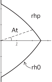
the assumption that |θ|≤π2−ε​a−2|\theta|\leq\tfrac{\pi}{2}-\varepsilon a^{-2} implies that (s⁡(n−s)CLOSE(s(n-s) remains a distance O⁡(ε)O(\varepsilon) from σ⁡(P)\sigma(P) for aa sufficiently large. The hypothesis of Lemma 5.2 is thus satisfied, yielding the estimate (5.1) with a CC that depends only on ε\varepsilon, η\eta, and r0r_{0}. To apply Lemma 5.3 to estimate the right-hand side of (5.1), we need to distinguish the terms according to the sign of H⁡(α,r3)H(\alpha,r_{3}). For large aa the sum is dominated by terms with H⁡(α,r3)>0H(\alpha,r_{3})>0, which occurs for α\alpha outside a certain neighborhood of the origin, as shown in Figure 5.
Refer to caption
Figure 5. The positive region for H⁡(α,r)H(\alpha,r), shown for r=1r=1.

Let x=A⁡(θ)x=A(\theta) be the implicit solution of the equation H⁡(x​ei​θ,r3)=0H(xe^{i\theta},r_{3})=0, so that H⁡(x​ei​θ,r3)>0H(xe^{i\theta},r_{3})>0 precisely when x>A⁡(θ)x>A(\theta). Given some δ>0\delta>0, we will subdivide the sum (5.1) by breaking at values where |α|=A⁡(θ)|\alpha|=A(\theta) and (1−δ)​A​(θ)(1-\delta)A(\theta), leaving us with three parts. The dominant part of the sum will be

Σ+:=∑l:|α|≥A⁡(θ)hn(l)log(1+Cλl(s)).\Sigma_{+}:=\sum_{l:\>|\alpha|\geq A(\theta)}h_{n}(l)\log\Bigl(1+C\lambda_{l}(s)\Bigr).

(Recall that α=(s−n2)/k\alpha=(s-\tfrac{n}{2})/k where k=l+(n−1)/2k=l+(n-1)/2.) For α\alpha in this range, assuming |arg⁡α|≤π2|\arg\alpha|\leq\tfrac{\pi}{2}, we apply Lemma 5.3 to obtain

(5.7) log⁡(1+C​λl​(s))≤k​H​(α,r3)+C​log⁡k\log(1+C\lambda_{l}(s))\leq kH(\alpha,r_{3})+C\log k

Using this estimate together with the asymptotic

hn​(l)=2​ln−1Γ⁡(n)​(1+O⁡(l−1)),h_{n}(l)=\frac{2l^{n-1}}{\Gamma(n)}(1+O(l^{-1})),

we have

(5.8) Σ+≤∑k≤a/A⁡(θ)(2​kn−1Γ⁡(n)+C​kn−2)​(k​H​(a​ei​θk,r3)+C​log⁡k).\Sigma_{+}\leq\sum_{k\leq a/A(\theta)}\left(\frac{2k^{n-1}}{\Gamma(n)}+Ck^{n-2}\right)\biggl(kH\Bigl(\frac{ae^{i\theta}}{k},r_{3}\Bigr)+C\log k\biggr).

(The sum could be restricted to k≥n−12k\geq\tfrac{n-1}{2}, but this would not improve the bound.) We can estimate H⁡(α,r3)=O⁡(|α|)H(\alpha,r_{3})=O(|\alpha|) with a constant that depends only on r3r_{3}. Thus

∑k≤a/A⁡(θ)kn−1​H​(a​ei​θk,r3)=O⁡(an).\sum_{k\leq a/A(\theta)}k^{n-1}H\Bigl(\frac{ae^{i\theta}}{k},r_{3}\Bigr)=O(a^{n}).

With this estimate, the sums over lower order terms in (5.8) are easily controlled, and we obtain

(5.9) Σ+≤2Γ⁡(n)​∑k≤a/A⁡(θ)kn​H​(a​ei​θk,r3)+C​an​log⁡a,\Sigma_{+}\leq\frac{2}{\Gamma(n)}\sum_{k\leq a/A(\theta)}k^{n}H\Bigl(\frac{ae^{i\theta}}{k},r_{3}\Bigr)+Ca^{n}\log a,

where CC depends only on ε\varepsilon, η\eta, and r0r_{0}.

Because H⁡(x​ei​θ,r)H(xe^{i\theta},r) is an increasing function of xx, the right-hand side of (5.9) is easily estimated by the corresponding integral,

Σ+≤2Γ⁡(n)​∫0aA⁡(θ)kn​H​(a​ei​θk,r3)​𝑑k+C​an​log⁡a.\Sigma_{+}\leq\frac{2}{\Gamma(n)}\int_{0}^{\frac{a}{A(\theta)}}k^{n}H\Bigl(\frac{ae^{i\theta}}{k},r_{3}\Bigr)\>dk+Ca^{n}\log a.

Making the substitution x=a/kx=a/k gives

Σ+≤2​an+1Γ⁡(n)​∫0∞[H⁡(x​ei​θ,r3)]+xn+2​𝑑x+C​an​log⁡a=b⁡(θ,r3)​an+1+C​an​log⁡a,\begin{split}\Sigma_{+}&\leq\frac{2a^{n+1}}{\Gamma(n)}\int_{0}^{\infty}\frac{[H(xe^{i\theta},r_{3})]_{+}}{x^{n+2}}\>dx+Ca^{n}\log a\\ &=b(\theta,r_{3})a^{n+1}+Ca^{n}\log a,\end{split}

with CC depending only on ε\varepsilon, η\eta, and r0r_{0}.

The middle term in (5.1) will be

Σ0:=∑l:(1−δ)​A​(θ)≤|α|≤A⁡(θ)hn(l)log(1+Cλl(s)).\Sigma_{0}:=\sum_{l:\>(1-\delta)A(\theta)\leq|\alpha|\leq A(\theta)}h_{n}(l)\log\Bigl(1+C\lambda_{l}(s)\Bigr).

The number of terms in this sum is O⁡(a​δ)O(a\delta), and we can control them using (5.7), noting also that H⁡(α,r3)=O⁡(δ)H(\alpha,r_{3})=O(\delta) for |α||\alpha| in the given range. Using an integral estimate as we did for Σ+\Sigma_{+}, we thus obtain

Σ0≤C​δ​an+1+C​an​log⁡a,\Sigma_{0}\leq C\delta a^{n+1}+Ca^{n}\log a,

where CC depends only on ε\varepsilon, η\eta, and r0r_{0}.

The final portion of the sum is

Σ−:=∑l:|α|≤(1−δ)​A​(θ)hn(l)log(1+Cλl(s)).\Sigma_{-}:=\sum_{l:\>|\alpha|\leq(1-\delta)A(\theta)}h_{n}(l)\log\Bigl(1+C\lambda_{l}(s)\Bigr).

We use the fact that H⁡(α,r3)≤−C​δH(\alpha,r_{3})\leq-C\delta in this range to estimate

log⁡(1+C​λl​(s))≤C​λl​(s)≤C​e−c​k.\log(1+C\lambda_{l}(s))\leq C\lambda_{l}(s)\leq Ce^{-ck}.

This implies

Σ−≤Cδ​e−c​a,\Sigma_{-}\leq C_{\delta}e^{-ca},

for some c>0c>0, where CδC_{\delta} depends on δ\delta as well as ε\varepsilon and the rjr_{j}’s.

Adding the three parts Σ+,Σ0,Σ−\Sigma_{+},\Sigma_{0},\Sigma_{-} of (5.1) together now yields

(5.10) log|τ⁡(n2+a​ei​θ)|≤b⁡(θ,r3)​an+1+C⁡(ε,η,r0)​[δ​an+1+an​log⁡a]+C⁡(ε,η,r0,δ)​e−c​a,\log|\tau(\tfrac{n}{2}+ae^{i\theta})|\leq b(\theta,r_{3})a^{n+1}+C(\varepsilon,\eta,r_{0})\bigl[\delta a^{n+1}+a^{n}\log a\bigr]+C(\varepsilon,\eta,r_{0},\delta)e^{-ca},

where we have made the dependence of the constants explicit. Since H⁡(α,r)H(\alpha,r) is a strictly increasing function of rr, we can absorb the δ​an+1\delta a^{n+1} term into the first term by assuming that δ\delta is small relative to η\eta and replacing r3r_{3} with r4=r0+4​ηr_{4}=r_{0}+4\eta. With this change, we obtain from (5.10) the estimate

(5.11) log⁡|τ⁡(n2+a​ei​θ)|an+1≤b⁡(θ,r0+4​η)+C⁡(ε,η,r0,δ)​a−1​log⁡a.\frac{\log|\tau(\tfrac{n}{2}+ae^{i\theta})|}{a^{n+1}}\leq b(\theta,r_{0}+4\eta)+C(\varepsilon,\eta,r_{0},\delta)a^{-1}\log a.

The constant C⁡(ε,η,r0,δ)C(\varepsilon,\eta,r_{0},\delta) may well blow up as η→0\eta\to 0. The best we can do here is to observe that (5.11) implies

lim supa→∞[log⁡|τ⁡(n2+a​ei​θ)|an+1−b⁡(θ,r0)]≤b⁡(θ,r0+4​η)−b⁡(θ,r0),\limsup_{a\to\infty}\left[\frac{\log|\tau(\tfrac{n}{2}+ae^{i\theta})|}{a^{n+1}}-b(\theta,r_{0})\right]\leq b(\theta,r_{0}+4\eta)-b(\theta,r_{0}),

for any η>0\eta>0. Since b⁡(θ,r)b(\theta,r) is uniformly continuous on [−π2,π2]×[r0,r0+1][-\tfrac{\pi}{2},\tfrac{\pi}{2}]\times[r_{0},r_{0}+1], we can now let η→0\eta\to 0 to obtain the claimed o⁡(an+1)o(a^{n+1}) estimate. ∎

Proof of Theorem 5.1.

For any ε>0\varepsilon>0, we can integrate the result from Proposition 5.4 over |θ|≤π2−ε​a−2|\theta|\leq\tfrac{\pi}{2}-\varepsilon a^{-2}, which gives,

∫|θ|≤π2−ε​a−2log⁡|τ⁡(n2+a​ei​θ)|​𝑑θ≤BP(2)​an+1+o⁡(an+1).\int_{|\theta|\leq\tfrac{\pi}{2}-\varepsilon a^{-2}}\log|\tau(\tfrac{n}{2}+ae^{i\theta})|\>d\theta\leq B_{P}^{(2)}a^{n+1}+o(a^{n+1}).

The factorization given by Proposition 3.1, together with the minimum modulus theorem (see e.g. [24, Thm. 8.71]), implies that for any δ>0\delta>0, there exists a sequence ri→∞r_{i}\to\infty such that

(5.12) |τ⁡(n2+ri​ei​θ)|≤Cδ​exp⁡(rin+1+δ),|\tau(\tfrac{n}{2}+r_{i}e^{i\theta})|\leq C_{\delta}\exp(r_{i}^{n+1+\delta}),

uniformly in θ\theta. In sectors of the form |θ|∈[π2−β,π2]|\theta|\in[\tfrac{\pi}{2}-\beta,\tfrac{\pi}{2}], where τ⁡(n2+a​ei​θ)\tau(\tfrac{n}{2}+ae^{i\theta}) is analytic, we can apply a Phragmén-Lindelöf argument, using (5.12), log⁡|τ⁡(s)|=0\log|\tau(s)|=0 for Re⁡s=n2\operatorname{Re}s=\tfrac{n}{2}, and the estimate from Proposition 5.4 for |θ|=π2−β|\theta|=\tfrac{\pi}{2}-\beta, to conclude that

|τ⁡(n2+a​ei​θ)|≤C​an+1,|\tau(\tfrac{n}{2}+ae^{i\theta})|\leq Ca^{n+1},

uniformly for |θ|∈[π2−β,π2]|\theta|\in[\tfrac{\pi}{2}-\beta,\tfrac{\pi}{2}]. Thus,

∫π2−ε​a−2≤|θ|≤π2log⁡|τ⁡(n2+a​ei​θ)|​𝑑θ≤C​ε​an−1.\int_{\frac{\pi}{2}-\varepsilon a^{-2}\leq|\theta|\leq\frac{\pi}{2}}\log|\tau(\tfrac{n}{2}+ae^{i\theta})|\>d\theta\leq C\varepsilon a^{n-1}.

∎

6. Examples

Suppose that X=ℍn+1X=\mathbb{H}^{n+1} and we consider a black box perturbation P=Δg+VP=\Delta_{g}+V, where both the metric gg and potential VV are spherically symmetric. The symmetry assumption guarantees that the perturbed Poisson kernel is “diagonalized” by spherical harmonics, in the sense that

EP​(s,r,ω,ω′)=∑l=0∞∑m=1hn​(l)al​(s,r)​Ylm​(ω)​Ylm​(ω′)¯,E_{P}(s;r,\omega,\omega^{\prime})=\sum_{l=0}^{\infty}\sum_{m=1}^{h_{n}(l)}a_{l}(s;r)Y_{l}^{m}(\omega)\overline{Y_{l}^{m}(\omega^{\prime})},

The coefficients al​(s,r)a_{l}(s;r) will satisfy (4.5) for r>r0r>r_{0} and are thus expressible in terms of Legendre functions. Following the convention of Olver, we use the Legendre Q-function in the form

(6.1) 𝐐νμ​(z):=e−μ​π​iΓ⁡(ν+μ+1)​Qνμ​(z),\mathbf{Q}_{\nu}^{\mu}(z):=\frac{e^{-\mu\pi i}}{\Gamma(\nu+\mu+1)}\>Q_{\nu}^{\mu}(z),

where Qνμ​(z)Q_{\nu}^{\mu}(z) is the standard definition. This makes 𝐐νμ​(z)\mathbf{Q}_{\nu}^{\mu}(z) an entire function of either μ\mu or ν\nu, which is much more convenient for identifying resonances. We can formulate the general solution of (4.5) for r>r0r>r_{0} as

(6.2) al​(s,r)=(sinh⁡r)−n−12​[Al​(s)​𝐐νk​(cosh⁡r)+Bl​(s)​𝐐−ν−1k​(cosh⁡r)],a_{l}(s;r)=(\sinh r)^{-\frac{n-1}{2}}\biggl[A_{l}(s)\mathbf{Q}_{\nu}^{k}(\cosh r)+B_{l}(s)\mathbf{Q}_{-\nu-1}^{k}(\cosh r)\biggr],

where

(6.3) k:=l+n−12,ν:=s−n+12.k:=l+\frac{n-1}{2},\qquad\nu:=s-\frac{n+1}{2}.

In particular examples, Al​(s)A_{l}(s) and Bl​(s)B_{l}(s) will be determined by matching ala_{l} and its first derivative to the corresponding solutions for r<r0r<r_{0}. The scattering matrix elements can be read off from the asymptotics of these solutions as r→∞r\to\infty, using

al​(s,r)∼cs​(ρn−s+ρs​[SP​(s)]l),a_{l}(s;r)\sim c_{s}\bigl(\rho^{n-s}+\rho^{s}[S_{P}(s)]_{l}\bigr),

in the same way that we found [S0​(s)]l[S_{0}(s)]_{l} in (4.8). Indeed, from the well-known asymptotic [19, eq. (12.09)]

(6.4) 𝐐νk​(z)=π12Γ⁡(ν+32)​(z2)−ν−1​(1+O⁡(z−2)),as ​z→∞,\mathbf{Q}_{\nu}^{k}(z)=\frac{\pi^{\frac{1}{2}}}{\Gamma(\nu+\tfrac{3}{2})}\Bigl(\frac{z}{2}\Bigr)^{-\nu-1}(1+O(z^{-2})),\qquad\text{as }z\to\infty,

we can see from (6.2) that the scattering matrix elements are given by

(6.5) [SP​(s)]l=−2n−2​s​Γ⁡(n2−s)Γ⁡(s−n2)​Al​(s)Bl​(s).[S_{P}(s)]_{l}=-2^{n-2s}\frac{\Gamma(\tfrac{n}{2}-s)}{\Gamma(s-\tfrac{n}{2})}\frac{A_{l}(s)}{B_{l}(s)}.

Consider the case where PP is the Laplacian for a spherical obstacle of radius r0r_{0} in ℍn+1\mathbb{H}^{n+1}. Imposing the Dirichlet boundary condition at r=r0r=r_{0} gives coefficients

As=𝐐−ν−1k​(cosh⁡r0),Bs=−𝐐νk​(cosh⁡r0).A_{s}=\mathbf{Q}_{-\nu-1}^{k}(\cosh r_{0}),\qquad B_{s}=-\mathbf{Q}_{\nu}^{k}(\cosh r_{0}).

In this case, from (6.5) we see that

(6.6) [SP​(s)]l=2n−2​s​Γ⁡(n2−s)Γ⁡(s−n2)​𝐐−ν−1k​(cosh⁡r0)𝐐νk​(cosh⁡r0).[S_{P}(s)]_{l}=2^{n-2s}\frac{\Gamma(\tfrac{n}{2}-s)}{\Gamma(s-\tfrac{n}{2})}\frac{\mathbf{Q}_{-\nu-1}^{k}(\cosh r_{0})}{\mathbf{Q}_{\nu}^{k}(\cosh r_{0})}.

With this observation we can give the:

Proof of Theorem 1.2.

Our goal is to show that

(6.7) 12​π​∫−π2π2log⁡|τ⁡(n2+a​ei​θ)|​𝑑θ∼Bn​(r0)​an+1.\frac{1}{2\pi}\int_{-\frac{\pi}{2}}^{\frac{\pi}{2}}\log|\tau(\tfrac{n}{2}+ae^{i\theta})|\>d\theta\sim B_{n}(r_{0})a^{n+1}.

In conjunction with Proposition 3.2 and Corollary 3.6, (6.7) would imply that

(n+1)​∫0aNP​(t)t​𝑑t∼BP​an+1,(n+1)\int_{0}^{a}\frac{N_{P}(t)}{t}\>dt\sim B_{P}a^{n+1},

and this is equivalent to the stated asymptotic for NP​(t)N_{P}(t).

Using (6.6) with (4.8) gives the relative scattering matrix elements,

[SP​(s)​S0​(s)−1]l=Γ⁡(l+n−s)Γ⁡(l+s)​𝐐−ν−1k​(cosh⁡r0)𝐐νk​(cosh⁡r0),[S_{P}(s)S_{0}(s)^{-1}]_{l}=\frac{\Gamma(l+n-s)}{\Gamma(l+s)}\frac{\mathbf{Q}_{-\nu-1}^{k}(\cosh r_{0})}{\mathbf{Q}_{\nu}^{k}(\cosh r_{0})},

with kk and ν\nu defined as in (6.3). With the connection formula [19, eq. (12.12)],

𝐐−ν−1k​(z)Γ⁡(k+ν+1)−𝐐νk​(z)Γ⁡(k−ν)=cos⁡(π​ν)​Pν−μ​(z),\frac{\mathbf{Q}_{-\nu-1}^{k}(z)}{\Gamma(k+\nu+1)}-\frac{\mathbf{Q}_{\nu}^{k}(z)}{\Gamma(k-\nu)}=\cos(\pi\nu)\>P_{\nu}^{-\mu}(z),

we can rewrite the coefficient in the form

(6.8) [SP​(s)​S0​(s)−1]l=1−cos⁡(π​ν)​Γ​(k−ν)​Pν−k​(cosh⁡r0)𝐐νk​(cosh⁡r0).[S_{P}(s)S_{0}(s)^{-1}]_{l}=1-\cos(\pi\nu)\>\Gamma(k-\nu)\frac{P_{\nu}^{-k}(\cosh r_{0})}{\mathbf{Q}_{\nu}^{k}(\cosh r_{0})}.

Now consider

log⁡|τ⁡(s)|=∑l=0∞hn​(l)​log⁡|[SP​(s)​S0​(s)−1]l|.\log|\tau(s)|=\sum_{l=0}^{\infty}h_{n}(l)\log\Bigl|[S_{P}(s)S_{0}(s)^{-1}]_{l}\Bigr|.

Defining α\alpha by k​α=s−n2k\alpha=s-\tfrac{n}{2}, we can use (6.8) to write this as

(6.9) log⁡|τ⁡(s)|=∑l=0∞hn​(l)​log⁡|1−ηk​(α)|,\log|\tau(s)|=\sum_{l=0}^{\infty}h_{n}(l)\log|1-\eta_{k}(\alpha)|,

where

ηk​(α):=sin⁡(π​k​α)​Γ​(k⁡(1−α)+12)​P−12+k​α−k​(cosh⁡r0)𝐐−12+k​αk​(cosh⁡r0).\eta_{k}(\alpha):=\sin(\pi k\alpha)\>\Gamma(k(1-\alpha)+\tfrac{1}{2})\>\frac{P_{-\frac{1}{2}+k\alpha}^{-k}(\cosh r_{0})}{\mathbf{Q}_{-\frac{1}{2}+k\alpha}^{k}(\cosh r_{0})}.

Assuming that |arg⁡α|≤π2−ε|\arg\alpha|\leq\tfrac{\pi}{2}-\varepsilon, Corollary A.3 gives the estimate

log⁡|ηk​(α)|≍|sin⁡(π​k​α)​Γ​(k⁡(1−α)+12)​Γ​(k​α+1)Γ⁡(k+1)|​ek​Re⁡[2​ϕ​(α,r0)−p⁡(α)−q⁡(α)],\log|\eta_{k}(\alpha)|\asymp\left|\frac{\sin(\pi k\alpha)\>\Gamma(k(1-\alpha)+\tfrac{1}{2})\Gamma(k\alpha+1)}{\Gamma(k+1)}\right|e^{k\operatorname{Re}[2\phi(\alpha,r_{0})-p(\alpha)-q(\alpha)]},

with constants depending only on ε\varepsilon. Applying Stirling’s formula and avoiding the poles by assuming |s−n2|∈ℕ|s-\tfrac{n}{2}|\in\mathbb{N} as in the proof of Lemma 5.3, we have

sin⁡(π​k​α)​Γ​(k⁡(1−α)+12)​Γ​(k​α+1)Γ⁡(k+1)=k​Re⁡[α​log⁡α−(α−1)​log⁡(α−1)]+O⁡(log⁡α)\frac{\sin(\pi k\alpha)\>\Gamma(k(1-\alpha)+\tfrac{1}{2})\Gamma(k\alpha+1)}{\Gamma(k+1)}=k\operatorname{Re}\Bigl[\alpha\log\alpha-(\alpha-1)\log(\alpha-1)\Bigr]+O(\log\alpha)

Since

Re⁡[2​ϕ​(α,r0)−p⁡(α)−q⁡(α)+α​log⁡α−(α−1)​log⁡(α−1)]=H⁡(α,r0),\operatorname{Re}\Bigl[2\phi(\alpha,r_{0})-p(\alpha)-q(\alpha)+\alpha\log\alpha-(\alpha-1)\log(\alpha-1)\Bigr]=H(\alpha,r_{0}),

the full estimate is

(6.10) log⁡|ηk​(α)|≍k​H​(α,r0)+O⁡(log⁡α).\log|\eta_{k}(\alpha)|\asymp kH(\alpha,r_{0})+O(\log\alpha).

As in the proof of Proposition 5.4 we divide the sum (6.9) into three pieces Σ+,Σ0\Sigma_{+},\Sigma_{0}, and Σ−\Sigma_{-}, with breaks at |α|=(1±δ)​A​(θ)|\alpha|=(1\pm\delta)A(\theta) for some δ>0\delta>0. The dominant piece is

Σ+:=∑l:|α|≥(1+δ)​A​(θ)hn(l)log|1−ηk(α)|\Sigma_{+}:=\sum_{l:\>|\alpha|\geq(1+\delta)A(\theta)}h_{n}(l)\log|1-\eta_{k}(\alpha)|

Using the lower bound from (6.10), but otherwise arguing as in the proof of Proposition 5.4, we have

Σ+≥b⁡(θ,r0)​an+1+O⁡(an​log⁡a)\Sigma_{+}\geq b(\theta,r_{0})a^{n+1}+O(a^{n}\log a)

The estimates on Σ0\Sigma_{0} and Σ−\Sigma_{-} are identical to those in Proposition 5.4:

Σ0≤c​δ​an+1+O⁡(an​log⁡a),\Sigma_{0}\leq c\delta a^{n+1}+O(a^{n}\log a),

and

Σ−=O⁡(e−c​a).\Sigma_{-}=O(e^{-ca}).

Hence we conclude that

log|τ⁡(n2+a​ei​θ)|≥(b⁡(θ,r0)−c​δ)​an+1+O⁡(an​log⁡a),\log|\tau(\tfrac{n}{2}+ae^{i\theta})|\geq(b(\theta,r_{0})-c\delta)a^{n+1}+O(a^{n}\log a),

for a∈ℕa\in\mathbb{N} and |θ|≤π2−ε|\theta|\leq\tfrac{\pi}{2}-\varepsilon, with constants that depend only on r0r_{0} and ε\varepsilon.

Integrating, over θ\theta, and using Proposition 5.4 to control the errors from |θ|∈[π2−ε,π2]|\theta|\in[\tfrac{\pi}{2}-\varepsilon,\tfrac{\pi}{2}], we obtain the estimate

12​π​∫−π2π2log|τ⁡(n2+a​ei​θ)|𝑑θ≥(BP(2)−ϵ)​an+1−Cr0,ϵ​an​log⁡a,\frac{1}{2\pi}\int_{-\frac{\pi}{2}}^{\frac{\pi}{2}}\log|\tau(\tfrac{n}{2}+ae^{i\theta})|\>d\theta\geq(B_{P}^{(2)}-\epsilon)a^{n+1}-C_{r_{0},\epsilon}a^{n}\log a,

valid for any ϵ>0\epsilon>0. (This ϵ\epsilon combines the terms proportional to ε\varepsilon and δ\delta from above.) In combination with Theorem 5.1, this proves (6.7). ∎

With some care, the explicit scattering matrix provided by (6.5) can be used to compute resonances. Scattering poles and zeros are defined a renormalized scattering matrix S~P​(s)\tilde{S}_{P}(s), in which the infinite rank poles and zeros coming from the gamma functions are removed,

S~P​(s):=Γ⁡(s−n2)Γ⁡(n2−s)​SP​(s).\tilde{S}_{P}(s):=\frac{\Gamma(s-\tfrac{n}{2})}{\Gamma(\tfrac{n}{2}-s)}S_{P}(s).

The scattering multiplicity is then defined by

νP​(ζ):=−tr⁡[Resζ⁡S~P′​(s)​S~P​(s)−1].\nu_{P}(\zeta):=-\operatorname{tr}\bigl[\operatorname{Res}_{\zeta}\tilde{S}_{P}^{\prime}(s)\tilde{S}_{P}(s)^{-1}\bigr].

For ℍn+1\mathbb{H}^{n+1}, the connection between scattering multiplicities and resonances is given by [14, 3, 11]

νP​(ζ)=mP​(ζ)−mP​(n−ζ)+{0n​ odd∑l∈ℕ(𝟙n/2−l​(ζ)−𝟙n/2+l​(ζ))​hn+1​(l)n​ even\nu_{P}(\zeta)=m_{P}(\zeta)-m_{P}(n-\zeta)+\begin{cases}0&n\text{ odd}\\ \sum_{l\in\mathbb{N}}\Bigl(\mathbbm{1}_{n/2-l}(\zeta)-\mathbbm{1}_{n/2+l}(\zeta)\Bigr)h_{n+1}(l)&n\text{ even}\end{cases}

For Re⁡ζ<n2\operatorname{Re}\zeta<\tfrac{n}{2}, the term mP​(n−ζ)m_{P}(n-\zeta) plays a role only if PP has discrete spectrum. In the examples that we will consider explicitly, n=1n=1 and the discrete spectrum is empty. For these cases, the resonances are precisely the poles of the S~P​(s)\tilde{S}_{P}(s).

Consider first the spherical obstacle of radius r0r_{0} in ℍ2\mathbb{H}^{2}, for which the scattering matrix is given by (6.6). From this expression we can read off the resonance set

ℛP=⋃k∈ℤ{s:𝐐s−1k​(cosh⁡r0)=0}.\mathcal{R}_{P}=\bigcup_{k\in\mathbb{Z}}\bigl\{s:\mathbf{Q}^{k}_{s-1}(\cosh r_{0})=0\bigr\}.

Figures 2 and 3 were thus obtained through numerical computation of zeroes of the Legendre Q-function.

As a second example, we consider scattering in ℍ2\mathbb{H}^{2} by a radial step potential of the form

V⁡(r)={cr≤r0,0r>r0.V(r)=\begin{cases}c&r\leq r_{0},\\ 0&r>r_{0}.\end{cases}

In this case, with P=Δ0+VP=\Delta_{0}+V, the coefficient solutions for r≤r0r\leq r_{0} are Legendre PP functions Pω⁡(s)−k​(r0)P^{-k}_{\omega(s)}(r_{0}), with

ω⁡(s):=−12+(s−12)2+c.\omega(s):=-\tfrac{1}{2}+\sqrt{(s-\tfrac{1}{2})^{2}+c}.

The corresponding resonance set is

(6.11) ℛP=⋃k∈ℤ{s:𝒲⁡[𝐐s−1k​(z),Pω⁡(s)−k​(z)]|z=cosh⁡r0=0}.\mathcal{R}_{P}=\bigcup_{k\in\mathbb{Z}}\Bigl\{s:\mathcal{W}\bigl[{\mathbf{Q}^{k}_{s-1}}(z),P^{-k}_{\omega(s)}(z)\bigr]\Big|_{z=\cosh r_{0}}=0\Bigr\}.

where 𝒲\mathcal{W} is the Wronskian. Resonance counting functions for c=1c=1 and c=5c=5, with r0=1r_{0}=1, are shown in Figure 6.

We should note that Theorem 1.1 does not apply to the step potential, because the lack of smoothness means that we cannot derive scattering phase asymptotics through Corollary 3.6. In view of the scattering phase asymptotics proved by Christiansen [4] in the black box Euclidean case, one might hope that the smoothness requirement in our case could be loosened. However, the technique of Robert used in [4] does not seem to be applicable to the conformally compact hyperbolic case. In any case, it is interesting to compare the putative upper bound suggested by Theorem 1.1 to the empirical results based on (6.11). For both of the cases shown in Figure 6, the constant from the theorem would be BP≈3.15B_{P}\approx 3.15. The numerical results thus suggest that NP​(t)N_{P}(t) satisfies an asymptotic with a constant significantly smaller than upper bound that Theorem 1.1 would predict.

Refer to caption
Figure 6. Resonance counting functions for radial step potentials in ℍ2\mathbb{H}^{2}.

Our final example is a “transparent” spherical obstacle. Let P=ΔgP=\Delta_{g} where

g={κ2​g0r<r0,g0r≥r0..g=\begin{cases}\kappa^{2}g_{0}&r<r_{0},\\ g_{0}&r\geq r_{0}.\end{cases}.

Then

ℛP=⋃k∈ℤ{s:𝒲⁡[𝐐s−1k​(r0),Pω⁡(s)−k​(r0)]=0},\mathcal{R}_{P}=\bigcup_{k\in\mathbb{Z}}\Bigl\{s:\mathcal{W}\bigl[{\mathbf{Q}^{k}_{s-1}}(r_{0}),P^{-k}_{\omega(s)}(r_{0})\bigr]=0\Bigr\},

where

ω⁡(s):=−12+κ2​s​(s−1)+14\omega(s):=-\tfrac{1}{2}+\sqrt{\kappa^{2}s(s-1)+\tfrac{1}{4}}

Figure 7 shows resonance counting functions for κ=12\kappa=\tfrac{1}{2} and κ=2\kappa=\sqrt{2}. Once again, Theorem 1.1 does not apply because of the lack of smoothness. However, in this case the predicted constants,

BP={2.75κ=12,3.70κ=2,B_{P}=\begin{cases}2.75&\kappa=\tfrac{1}{2},\\ 3.70&\kappa=\sqrt{2},\end{cases}

at least roughly match the observed behavior, so that one might believe that the theorem would give a sharp result if extended to this case.

Refer to caption
Figure 7. Resonance counting functions for transparent spherical obstacles in ℍ2\mathbb{H}^{2} with r0=1r_{0}=1.

Appendix A Legendre function estimates

In this section we will estimate the growth of the Legendre functions Pνk​(cosh⁡r)P_{\nu}^{k}(\cosh r) and 𝐐νk​(cosh⁡r)\mathbf{Q}_{\nu}^{k}(\cosh r) as k,|ν|→∞k,|\nu|\to\infty simultaneously. We wish to extract the leading asymptotic behavior, with error bounds uniform in α:=(ν+12)/k\alpha:=(\nu+\tfrac{1}{2})/k for Re⁡α≥0\operatorname{Re}\alpha\geq 0. The construction of these estimates leans heavily on techniques from Olver [19, §11].

Throughout this discussion we identify z=cosh⁡rz=\cosh r and switch freely between the two variables. Let

w⁡(z)=(sinh⁡r)​{P−12+k​α−k​(cosh⁡r), or𝐐−12+k​αk​(cosh⁡r).w(z)=(\sinh r)\>\begin{cases}P_{-\frac{1}{2}+k\alpha}^{-k}(\cosh r),&\text{ or}\\ \mathbf{Q}_{-\frac{1}{2}+k\alpha}^{k}(\cosh r).\\ \end{cases}

Then the Legendre equation reduces to

(A.1) ∂z2w=(k2​f+g)​w,\partial_{z}^{2}w=(k^{2}f+g)\>w,

with

(A.2) f⁡(r):=1+α2​sinh2⁡rsinh4⁡r,g⁡(r):=−sinh2⁡r+44​sinh4⁡r.f(r):=\frac{1+\alpha^{2}\sinh^{2}r}{\sinh^{4}r},\qquad g(r):=-\frac{\sinh^{2}r+4}{4\sinh^{4}r}.

If Re⁡α=0\operatorname{Re}\alpha=0 then the equation (A.1) has turning points (points where ff vanishes to first order) when α=±i/sinhr\alpha=\pm i/\sinh r. By conjugation, it suffices to assume Im⁡α≥0\operatorname{Im}\alpha\geq 0 and so we focus on the upper turning point. To obtain uniform estimates near this point, we introduce the complex variable ζ\zeta defined by integrating

(A.3) ζ​d​ζ=f​d​z,\sqrt{\zeta}\>d\zeta=\sqrt{f}\>dz,

starting from ζ=0\zeta=0 on the left and from z0=1−1/α2z_{0}=\sqrt{1-1/\alpha^{2}} (the turning point) on the right. Throughout this section we assume principal branches for the logs and square roots, under the restriction that arg⁡α∈[0,π/2]\arg\alpha\in[0,\pi/2].

Integrating both sides of (A.3) yields

(A.4) 23​ζ32=ϕ,\tfrac{2}{3}\zeta^{\frac{3}{2}}=\phi,

where

(A.5) ϕ⁡(α,r):=∫cosh−1⁡z0r1+α2​sinh2⁡tsinh⁡t​𝑑t=α​log⁡(α​cosh⁡r+1+α2​sinh2⁡rα2−1)+12​log⁡[cosh⁡r−1+α2​sinh2⁡rcosh⁡r+1+α2​sinh2⁡r].\begin{split}\phi(\alpha,r)&:=\int_{\cosh^{-1}z_{0}}^{r}\frac{\sqrt{1+\alpha^{2}\sinh^{2}t}}{\sinh t}\>dt\\ &=\alpha\log\left(\frac{\alpha\cosh r+\sqrt{1+\alpha^{2}\sinh^{2}r}}{\sqrt{\alpha^{2}-1}}\right)+\frac{1}{2}\log\left[\frac{\cosh r-\sqrt{1+\alpha^{2}\sinh^{2}r}}{\cosh r+\sqrt{1+\alpha^{2}\sinh^{2}r}}\right].\end{split}

The expression (A.5) is well-defined by principal branches for arg⁡α∈(0,π/2]\arg\alpha\in(0,\pi/2], and we extend the definition to the positive real axis by continuity. (At the apparent singularity at α=1\alpha=1, this extension yields ϕ⁡(1,r)=log⁡sinh⁡r\phi(1,r)=\log\sinh r.)

The region of interest, namely arg⁡α∈[0,π/2]\arg\alpha\in[0,\pi/2] and r≥0r\geq 0, corresponds to the sector arg⁡ϕ∈[−π,π2]\arg\phi\in[-\pi,\tfrac{\pi}{2}], as illustrated in Figure 8. Figure 9 show the corresponding picture for ζ\zeta, and illustrates in particular how passing from ϕ\phi to ζ\zeta resolves the singularity at the turning point.

Refer to caption
Figure 8. Trajectories of ϕ⁡(α,⋅)\phi(\alpha,\cdot) with |α|=2|\alpha|=2 and θ=arg⁡α\theta=\arg\alpha. The turning point occurs at the origin.
Refer to caption
Figure 9. Trajectories of ζ⁡(α,⋅)\zeta(\alpha,\cdot) with |α|=2|\alpha|=2 and θ=arg⁡α\theta=\arg\alpha.

For future reference, we note that ϕ\phi satisfies the equation

(A.6) ∂rϕ=f​sinh⁡r,\partial_{r}\phi=\sqrt{f}\>\sinh r,

implying in particular that Re∂rϕ≥0\operatorname{Re}\partial_{r}\phi\geq 0. The fact that Re⁡ϕ\operatorname{Re}\phi is an increasing function of rr will be important later, and is not so evident from (A.5).

The asymptotics of ϕ⁡(α,⋅)\phi(\alpha,\cdot) will also play a crucial role. As r→0r\to 0, we have

(A.7) ϕ⁡(α,r)=log⁡(r2)+p⁡(α)+O⁡(r2),\phi(\alpha,r)=\log\left(\frac{r}{2}\right)+p(\alpha)+O(r^{2}),

where

(A.8) p⁡(α):=α2​log⁡(α+1α−1)+12​log⁡(1−α2),p(\alpha):=\frac{\alpha}{2}\log\left(\frac{\alpha+1}{\alpha-1}\right)+\frac{1}{2}\log(1-\alpha^{2}),

And as r→∞r\to\infty, we have

(A.9) ϕ⁡(α,r)=α​r+q⁡(α)+O⁡(r−2),\phi(\alpha,r)=\alpha r+q(\alpha)+O(r^{-2}),

where

(A.10) q⁡(α):=α​log⁡(αα2−1)+12​log⁡(1−α1+α),q(\alpha):=\alpha\log\left(\frac{\alpha}{\sqrt{\alpha^{2}-1}}\right)+\frac{1}{2}\log\left(\frac{1-\alpha}{1+\alpha}\right),
Proposition A.1.

Assuming that k>0k>0, arg⁡α∈[0,π2]\arg\alpha\in[0,\tfrac{\pi}{2}] and r∈[0,∞)r\in[0,\infty), we have

(A.11) P−12+k​α−k​(cosh⁡r)=2​π12Γ⁡(k+1)​k16​ζ14​eπ​i6[1+α2​sinh2⁡r]14​e−k​p​(α)​[Ai⁡(k23​e2​π​i3​ζ)+h1​(k,α,r)],P_{-\frac{1}{2}+k\alpha}^{-k}(\cosh r)=\frac{2\pi^{\frac{1}{2}}}{\Gamma(k+1)}\frac{k^{\frac{1}{6}}\zeta^{\frac{1}{4}}e^{\frac{\pi i}{6}}}{\bigl[1+\alpha^{2}\sinh^{2}r\bigr]^{\frac{1}{4}}}\>e^{-kp(\alpha)}\Bigl[{\rm Ai}\bigl(k^{\frac{2}{3}}e^{\frac{2\pi i}{3}}\zeta\bigr)+h_{1}(k,\alpha,r)\Bigr],

and

(A.12) 𝐐−12+k​αk​(cosh⁡r)=2​πΓ⁡(k​α+1)​k16​ζ14​(α2)12[1+α2​sinh2⁡r]14​ek​q​(α)​[Ai⁡(k23​ζ)+h0​(k,α,r)],\mathbf{Q}_{-\frac{1}{2}+k\alpha}^{k}(\cosh r)=\frac{2\pi}{\Gamma(k\alpha+1)}\frac{k^{\frac{1}{6}}\zeta^{\frac{1}{4}}(\frac{\alpha}{2})^{\frac{1}{2}}}{\bigl[1+\alpha^{2}\sinh^{2}r\bigr]^{\frac{1}{4}}}\>e^{kq(\alpha)}\Bigl[{\rm Ai}\bigl(k^{\frac{2}{3}}\zeta\bigr)+h_{0}(k,\alpha,r)\Bigr],

where ζ\zeta is defined by (A.4) and (A.5), p⁡(α)p(\alpha) and q⁡(α)q(\alpha) are defined in (A.8) and (A.10), respectively. The error terms satisfy

(A.13) |k16​ζ14​h1​(k,α,r)|≤C​ek​Re⁡ϕ​k−1​(1+|α|−23),|k16​ζ14​h0​(k,α,r)|≤C​e−k​Re⁡ϕ​k−1​(1+|α|−23).\begin{split}|k^{\frac{1}{6}}\zeta^{\frac{1}{4}}h_{1}(k,\alpha,r)|&\leq Ce^{k\operatorname{Re}\phi}k^{-1}\Bigl(1+|\alpha|^{-\frac{2}{3}}\Bigr),\\ |k^{\frac{1}{6}}\zeta^{\frac{1}{4}}h_{0}(k,\alpha,r)|&\leq Ce^{-k\operatorname{Re}\phi}k^{-1}\Bigl(1+|\alpha|^{-\frac{2}{3}}\Bigr).\end{split}

with CC independent of both α\alpha and rr.

Proof.

If we set W=(f/ζ)1/4​wW=(f/\zeta)^{1/4}w, then the equation (A.1) transforms to:

(A.14) ∂ζ2W=(k2​ζ+ψ)​W,\partial_{\zeta}^{2}W=(k^{2}\zeta+\psi)W,

a perturbed version of the Airy equation, with the extra term given by

(A.15) ψ=ζ4​f2​∂z2f−5​ζ16​f3​(∂zf)2+ζ​gf+516​ζ2.\psi=\frac{\zeta}{4f^{2}}\partial_{z}^{2}f-\frac{5\zeta}{16f^{3}}(\partial_{z}f)^{2}+\frac{\zeta g}{f}+\frac{5}{16\zeta^{2}}.

Following Olver [19, Thm. 11.9.1], we consider solutions of the form

(A.16) Wσ=Ai⁡(k23​e2​π​i​σ3​ζ)+hσ​(k,α,r),W_{\sigma}={\rm Ai}(k^{\frac{2}{3}}e^{\frac{2\pi i\sigma}{3}}\zeta)+h_{\sigma}(k,\alpha,r),

for σ=−1,0,1\sigma=-1,0,1, where the error terms satisfy

(A.17) ∂ζ2hσ−k2​ζ​hσ=ψ⁡[hσ+Ai⁡(k23​e2​π​i​σ3​ζ)],\partial_{\zeta}^{2}h_{\sigma}-k^{2}\zeta h_{\sigma}=\psi\>\Bigl[h_{\sigma}+{\rm Ai}(k^{\frac{2}{3}}e^{\frac{2\pi i\sigma}{3}}\zeta)\Bigr],

Let us focus first on the Legendre PP-function. As |w|→∞|w|\to\infty, the Airy function Ai⁡(w){\rm Ai}(w) is exponentially decreasing for |arg⁡w|<π3|\arg w|<\tfrac{\pi}{3} and exponentially increasing for |arg⁡w|∈(π3,π]|\arg w|\in(\tfrac{\pi}{3},\pi]. Since P−12+k​α−k​(cosh⁡r)P_{-\frac{1}{2}+k\alpha}^{-k}(\cosh r) is recessive at zero, and r→0r\to 0 corresponds to ζ→e−2​π​i3​∞\zeta\to e^{-\frac{2\pi i}{3}}\infty, we choose the solution W1W_{1} from (A.16). The assumption that the solution is recessive as r→0r\to 0 implies boundary conditions,

(A.18) h1|r=0=∂rh1|r=0=0,h_{1}|_{r=0}=\partial_{r}h_{1}|_{r=0}=0,

which we must impose on (A.17). To identify the Legendre PP function with a multiple of W1W_{1}, we compare the well-known asymptotic

P−12+k​α−k​(cosh⁡r)=1Γ⁡(k+1)​(r2)k​(1+O⁡(r2)),P_{-\frac{1}{2}+k\alpha}^{-k}(\cosh r)=\frac{1}{\Gamma(k+1)}\Bigl(\frac{r}{2}\Bigr)^{k}(1+O(r^{2})),

to the behavior of the ansatz

(sinh⁡r)−1​(ζ/f)14​W1=ζ14[1+α2​sinh2⁡r]14​(Ai⁡(k23​e2​π​i3​ζ)+h1​(k,α,r)).(\sinh r)^{-1}(\zeta/f)^{\frac{1}{4}}W_{1}=\frac{\zeta^{\frac{1}{4}}}{[1+\alpha^{2}\sinh^{2}r]^{\frac{1}{4}}}\Bigl({\rm Ai}(k^{\frac{2}{3}}e^{\frac{2\pi i}{3}}\zeta)+h_{1}(k,\alpha,r)\Bigr).

Away from the negative real axis, the Airy function has the asymptotic behavior [19, eq. (4.4.03)]

(A.19) Ai⁡(w)=12​π12​w−14​exp⁡(−23​w32)​[1+O⁡(|w|−32)],{\rm Ai}(w)=\frac{1}{2\pi^{\frac{1}{2}}}w^{-\frac{1}{4}}\exp\bigl(-\tfrac{2}{3}w^{\frac{3}{2}}\bigr)\bigl[1+O(|w|^{-\frac{3}{2}})\bigr],

uniformly for |arg⁡w|≤π−δ|\arg w|\leq\pi-\delta, with a constant that depends only on δ>0\delta>0. To cover the negative real axis we have also [19, eq. (4.4.05)],

(A.20) Ai⁡(w)=1π12​(−w)−14​cos⁡(23​(−w)32−π4)​[1+O⁡(|w|−32)],{\rm Ai}(w)=\frac{1}{\pi^{\frac{1}{2}}}(-w)^{-\frac{1}{4}}\cos\Bigl(\tfrac{2}{3}(-w)^{\frac{3}{2}}-\tfrac{\pi}{4}\Bigr)\bigl[1+O(|w|^{-\frac{3}{2}})\bigr],

uniformly for |arg⁡w|∈[π3+δ,π]|\arg w|\in[\tfrac{\pi}{3}+\delta,\pi]. (These estimates agree where they overlap.)

As r→0r\to 0, we have e2​π​i3​ζ→+∞e^{\frac{2\pi i}{3}}\zeta\to+\infty, which is in the range covered by (A.19). Along with the asymptotic behavior of ζ\zeta deduced from (A.7), this yields

ζ14​Ai​(k23​e2​π​i3​ζ)∼k−16​e−π​i62​π12​ek​p​(α)​(r2)kas ​r→0.\zeta^{\frac{1}{4}}{\rm Ai}(k^{\frac{2}{3}}e^{\frac{2\pi i}{3}}\zeta)\sim k^{-\frac{1}{6}}\frac{e^{-\frac{\pi i}{6}}}{2\pi^{\frac{1}{2}}}e^{kp(\alpha)}\left(\frac{r}{2}\right)^{k}\quad\text{as }r\to 0.

Thus for the Legendre PP-function we find

P−12+k​α−k​(cosh⁡r)=2​π12​k16​eπ​i6​e−k​p​(α)Γ⁡(k+1)​(sinh⁡r)−1​(ζ/f)14​W1,P_{-\frac{1}{2}+k\alpha}^{-k}(\cosh r)=2\pi^{\frac{1}{2}}k^{\frac{1}{6}}e^{\frac{\pi i}{6}}\frac{e^{-kp(\alpha)}}{\Gamma(k+1)}(\sinh r)^{-1}(\zeta/f)^{\frac{1}{4}}W_{1},

which proves (A.11).

To complete the analysis of the PP case, it remains to control the size of the error term h1​(k,α,r)h_{1}(k,\alpha,r). The error bounds may be derived as in the proof of [19, Thm. 11.9.1], starting from the differential equation (A.17) satisfied by h1h_{1}. Using the boundary condition (A.18), we can apply variation of parameters to transform this to an integral equation,

h1(k,α,r)=−2​π​ei​π6k23∫0rK1(r,r′)ψ(r′)[h1(k,α,r′)+Ai(k23e2​π​i3ζ(r′))]f(r′)12sinhr′ζ​(r′)12dr′,h_{1}(k,\alpha,r)=-\frac{2\pi e^{\frac{i\pi}{6}}}{k^{\frac{2}{3}}}\int_{0}^{r}K_{1}(r,r^{\prime})\psi(r^{\prime})\>[h_{1}(k,\alpha,r^{\prime})+{\rm Ai}(k^{\frac{2}{3}}e^{\frac{2\pi i}{3}}\zeta(r^{\prime}))]\>\frac{f(r^{\prime})^{\frac{1}{2}}\sinh r^{\prime}}{\zeta(r^{\prime})^{\frac{1}{2}}}\>dr^{\prime},

where

K1​(r,r′):=Ai⁡(k23​e2​π​i3​ζ​(r′))​Ai​(k23​ζ​(r))−Ai⁡(k23​ζ​(r′))​Ai​(k23​e2​π​i3​ζ​(r)).K_{1}(r,r^{\prime}):={\rm Ai}(k^{\frac{2}{3}}e^{\frac{2\pi i}{3}}\zeta(r^{\prime})){\rm Ai}(k^{\frac{2}{3}}\zeta(r))-{\rm Ai}(k^{\frac{2}{3}}\zeta(r^{\prime})){\rm Ai}(k^{\frac{2}{3}}e^{\frac{2\pi i}{3}}\zeta(r)).

Then, using the method of successive approximations as in [19, Thm. 6.10.2], together with the bounds on the Airy function and its derivatives developed in [19, §11.8], we obtain the bound,

(A.21) |k16​ζ14​h1|≤C​ek​Re⁡ϕ​(ec​k−1​Ψ1​(r)−1),\Bigl|k^{\frac{1}{6}}\>\zeta^{\frac{1}{4}}h_{1}\Bigr|\leq Ce^{k\operatorname{Re}\phi}\Bigl(e^{ck^{-1}\Psi_{1}(r)}-1\Bigr),

where

(A.22) Ψ1(r):=∫0r|ψf12ζ−12|sinhr′dr′.\Psi_{1}(r):=\int_{0}^{r}\left|\psi f^{\frac{1}{2}}\zeta^{-\frac{1}{2}}\right|\>\sinh r^{\prime}\>dr^{\prime}.

Using (A.2) and (A.15), direct computation shows that

(A.23) ψ​f12​ζ−12=ζ12​[α4​sinh2⁡r−4​α2​cosh2⁡r+14​(1+α2​sinh2⁡r)52]+516​(1+α2​sinh2⁡r)12ζ52​sinh2⁡r.\psi f^{\frac{1}{2}}\zeta^{-\frac{1}{2}}=\zeta^{\frac{1}{2}}\left[\frac{\alpha^{4}\sinh^{2}r-4\alpha^{2}\cosh^{2}r+1}{4(1+\alpha^{2}\sinh^{2}r)^{\frac{5}{2}}}\right]+\frac{5}{16}\frac{(1+\alpha^{2}\sinh^{2}r)^{\frac{1}{2}}}{\zeta^{\frac{5}{2}}\sinh^{2}r}.

Because we require estimates that are uniform in both α\alpha and rr, the analysis of (A.23) is somewhat complicated. For some small c>0c>0, we will break the estimation into 3 different zones as described below. We use the notation A≍BA\asymp B to mean that the ratio A/BA/B is bounded above and below by positive constants that do not depend on α\alpha or rr.

Zone 1: Assume that |1+α2​sinh2⁡r|≥c|1+\alpha^{2}\sinh^{2}r|\geq c and |α|≥1|\alpha|\geq 1. The first term in the formula (A.5) for ϕ\phi dominates for large rr and the second term for small rr. We can thus derive the bounds,

|ϕ|≍{−log⁡|α|​rfor ​|α|​sinh⁡r≤12|α|​rfor ​|α|​sinh⁡r≥12,|\phi|\asymp\begin{cases}-\log|\alpha|r&\text{for }|\alpha|\sinh r\leq\tfrac{1}{2}\\ |\alpha|r&\text{for }|\alpha|\sinh r\geq\tfrac{1}{2},\end{cases}

Using this to estimate ζ=(32​ϕ)23\zeta=(\tfrac{3}{2}\phi)^{\frac{2}{3}} in (A.23) gives

|ψ​f12​ζ−12|​sinh⁡r≤{C1​|α|2​(−log⁡|α|​r)13​r+C2​(−log⁡|α|​r)−53​r−1for ​|α|​sinh⁡r≤12,C1​|α|−23​r13​e−2​r+C2​|α|−23​r−53for ​|α|​sinh⁡r≥12.\left|\psi f^{\frac{1}{2}}\zeta^{-\frac{1}{2}}\right|\>\sinh r\leq\begin{cases}C_{1}|\alpha|^{2}(-\log|\alpha|r)^{\frac{1}{3}}r+C_{2}(-\log|\alpha|r)^{-\frac{5}{3}}r^{-1}&\text{for }|\alpha|\sinh r\leq\tfrac{1}{2},\\ C_{1}|\alpha|^{-\frac{2}{3}}r^{\frac{1}{3}}e^{-2r}+C_{2}|\alpha|^{-\frac{2}{3}}r^{-\frac{5}{3}}&\text{for }|\alpha|\sinh r\geq\tfrac{1}{2}.\end{cases}

It is then relatively straightforward to control the contribution of these terms to (A.22). For |α|≥1|\alpha|\geq 1, we obtain

(A.24) ∫|1+α2​sinh2⁡r|≥c|ψ​f12​ζ−12|​sinh⁡r​𝑑r≤C,\int_{|1+\alpha^{2}\sinh^{2}r|\geq c}\left|\psi f^{\frac{1}{2}}\zeta^{-\frac{1}{2}}\right|\>\sinh r\>dr\leq C,

for some CC that depends on cc but not on α\alpha.

Zone 2: Assume that |1+α2​sinh2⁡r|≥c|1+\alpha^{2}\sinh^{2}r|\geq c and |α|≤1|\alpha|\leq 1. In this case we claim that

|ϕ|≍{|log⁡(1−e−r)|for ​|α|​sinh⁡r≤12|α|​(r+log⁡2​|α|)for ​|α|​sinh⁡r≥12,|\phi|\asymp\begin{cases}|\log(1-e^{-r})|&\text{for }|\alpha|\sinh r\leq\tfrac{1}{2}\\ |\alpha|\bigl(r+\log 2|\alpha|\bigr)&\text{for }|\alpha|\sinh r\geq\tfrac{1}{2},\end{cases}

Using these in conjunction with (A.23) then gives

|ψ​f12​ζ−12|​sinh⁡r≤{C1​|log⁡(1−e−r)|13​sinh⁡r+C2​|log⁡(1−e−r)|−53​(sinh⁡r)−1for ​|α|​sinh⁡r≤12,C1​|α|−23​(r+log⁡2​|α|)13​e−2​r+C2​|α|−23​(r+log⁡2​|α|)−53for ​|α|​sinh⁡r≥12.\left|\psi f^{\frac{1}{2}}\zeta^{-\frac{1}{2}}\right|\>\sinh r\leq\begin{cases}C_{1}|\log(1-e^{-r})|^{\frac{1}{3}}\sinh r+C_{2}|\log(1-e^{-r})|^{-\frac{5}{3}}(\sinh r)^{-1}&\text{for }|\alpha|\sinh r\leq\tfrac{1}{2},\\ C_{1}|\alpha|^{-\frac{2}{3}}(r+\log 2|\alpha|)^{\frac{1}{3}}e^{-2r}+C_{2}|\alpha|^{-\frac{2}{3}}\bigl(r+\log 2|\alpha|\bigr)^{-\frac{5}{3}}&\text{for }|\alpha|\sinh r\geq\tfrac{1}{2}.\end{cases}

For |α|≤1|\alpha|\leq 1, we obtain

(A.25) ∫|1+α2​sinh2⁡r|≥c|ψ​f12​ζ−12|​sinh⁡r​𝑑r≤C​|α|−23,\int_{|1+\alpha^{2}\sinh^{2}r|\geq c}\left|\psi f^{\frac{1}{2}}\zeta^{-\frac{1}{2}}\right|\>\sinh r\>dr\leq C|\alpha|^{-\frac{2}{3}},

for some CC that depends on cc but not on α\alpha.

Zone 3: Assume that |1+α2​sinh2⁡r|≤c|1+\alpha^{2}\sinh^{2}r|\leq c. This puts us near the turning point. It is convenient to use the z=cosh⁡rz=\cosh r variable here. The turning point occurs at the point

z0:=1−α−2,z_{0}:=\sqrt{1-\alpha^{-2}},

which lies near the path of integration for (A.22) only when arg⁡α\arg\alpha is close to π2\tfrac{\pi}{2}. Note that

1+α2​sinh2⁡r=α2​(z2−z02),1+\alpha^{2}\sinh^{2}r=\alpha^{2}(z^{2}-z_{0}^{2}),

so that the assumption |1+α2​sinh2⁡r|≤c|1+\alpha^{2}\sinh^{2}r|\leq c translates to

|z−z0|={O⁡(|α|−1)for ​|α|≤1O⁡(|α|−2)for ​|α|≥1|z-z_{0}|=\begin{cases}O(|\alpha|^{-1})&\text{for }|\alpha|\leq 1\\ O(|\alpha|^{-2})&\text{for }|\alpha|\geq 1\end{cases}

To obtain estimates near the turning point, we introduce the functions

p⁡(z):=(fz−z0)12,q⁡(z)=ϕ(z−z0)32.p(z):=\left(\frac{f}{z-z_{0}}\right)^{\frac{1}{2}},\quad q(z)=\frac{\phi}{(z-z_{0})^{\frac{3}{2}}}.

By rewriting p⁡(z)p(z) in the form

p⁡(z)=α​z+z0z2−1,p(z)=\frac{\alpha\sqrt{z+z_{0}}}{z^{2}-1},

we can easily obtain estimates,

(A.26) |p(k)​(z)|≍{|α|52+kfor ​|α|≤1​ and |z−z0|=O⁡(|α|−1),|α|3+2​kfor ​|α|≥1​ and |z−z0|=O⁡(|α|−2).|p^{(k)}(z)|\asymp\begin{cases}|\alpha|^{\frac{5}{2}+k}&\text{for }|\alpha|\leq 1\text{ and }|z-z_{0}|=O(|\alpha|^{-1}),\\ |\alpha|^{3+2k}&\text{for }|\alpha|\geq 1\text{ and }|z-z_{0}|=O(|\alpha|^{-2}).\end{cases}

Using the definition of ϕ\phi as ∫z0zf​𝑑z\int_{z_{0}}^{z}\sqrt{f}\>dz, we can write q⁡(z)q(z) in the form

q⁡(z)=∫01t12​p​(z0+t⁡(z−z0))​𝑑t.q(z)=\int_{0}^{1}t^{\frac{1}{2}}p(z_{0}+t(z-z_{0}))\>dt.

Then from (A.26) we can derive estimates of the same form for q⁡(z)q(z),

(A.27) |q(k)​(z)|≍{|α|52+kfor ​|α|≤1​ and |z−z0|=O⁡(|α|−1),|α|3+2​kfor ​|α|≥1​ and |z−z0|=O⁡(|α|−2).|q^{(k)}(z)|\asymp\begin{cases}|\alpha|^{\frac{5}{2}+k}&\text{for }|\alpha|\leq 1\text{ and }|z-z_{0}|=O(|\alpha|^{-1}),\\ |\alpha|^{3+2k}&\text{for }|\alpha|\geq 1\text{ and }|z-z_{0}|=O(|\alpha|^{-2}).\end{cases}

Using (A.26) and (A.27), with the fact that f/ζ=p2​(32​q)−23f/\zeta=p^{2}(\tfrac{3}{2}q)^{-\frac{2}{3}} and the formula for ψ\psi given in (A.15), we obtain

|ψ​f12​ζ−12|≤{O⁡(|α|13)for ​|α|≤1​ and |z−z0|=O⁡(|α|−1),O⁡(|α|2)for ​|α|≥1​ and |z−z0|=O⁡(|α|−2).\left|\psi f^{\frac{1}{2}}\zeta^{-\frac{1}{2}}\right|\leq\begin{cases}O(|\alpha|^{\frac{1}{3}})&\text{for }|\alpha|\leq 1\text{ and }|z-z_{0}|=O(|\alpha|^{-1}),\\ O(|\alpha|^{2})&\text{for }|\alpha|\geq 1\text{ and }|z-z_{0}|=O(|\alpha|^{-2}).\end{cases}

For |α|≤1|\alpha|\leq 1, the result is

(A.28) ∫|z−z0|≤C​|α|−1|ψ​f12​ζ−12|​𝑑z=O⁡(|α|−23),\int_{|z-z_{0}|\leq C|\alpha|^{-1}}\left|\psi f^{\frac{1}{2}}\zeta^{-\frac{1}{2}}\right|\>dz=O(|\alpha|^{-\frac{2}{3}}),

For |α|≥1|\alpha|\geq 1 the corresponding estimate is

(A.29) ∫|z−z0|≤C​|α|−2|ψ​f12​ζ−12|​𝑑z=O⁡(1).\int_{|z-z_{0}|\leq C|\alpha|^{-2}}\left|\psi f^{\frac{1}{2}}\zeta^{-\frac{1}{2}}\right|\>dz=O(1).

Now we can combine the estimates of contributions to Ψ⁡(r)\Psi(r) from all three zones, namely (A.24), (A.25), (A.28), and (A.29), to obtain

(A.30) |Ψ1​(r)|≤C⁡(1+|α|−23),|\Psi_{1}(r)|\leq C(1+|\alpha|^{-\frac{2}{3}}),

for arg⁡α∈[0,π2]\arg\alpha\in[0,\tfrac{\pi}{2}] and r∈[0,∞)r\in[0,\infty), with CC independent of both rr and α\alpha. Applying the resulting estimate of Ψ⁡(r)\Psi(r) in (A.21) then gives

|k16​ζ14​h1|≤C​k−1​(1+|α|−23)​ek​Re⁡ϕ.\Bigl|k^{\frac{1}{6}}\>\zeta^{\frac{1}{4}}h_{1}\Bigr|\leq Ck^{-1}\Bigl(1+|\alpha|^{-\frac{2}{3}}\Bigr)e^{k\operatorname{Re}\phi}.

This completes the error analysis in the PP case.

We turn now to the Legendre QQ-function and the proof of (A.12). We want the solution to be recessive at r=∞r=\infty, so we set σ=0\sigma=0 in the ansatz (A.16) and impose the condition

(A.31) h0=O⁡(r−2), as ​r→∞.h_{0}=O(r^{-2}),\quad\text{ as }r\to\infty.

Using (A.9) and (A.19) we have

ζ14[1+α2​sinh2⁡r]14​Ai​(k23​ζ)∼k−16​(α2)−122​π12​e−(k​α+12)​r,\frac{\zeta^{\frac{1}{4}}}{[1+\alpha^{2}\sinh^{2}r]^{\frac{1}{4}}}{\rm Ai}(k^{\frac{2}{3}}\zeta)\sim\frac{k^{-\frac{1}{6}}(\frac{\alpha}{2})^{-\frac{1}{2}}}{2\pi^{\frac{1}{2}}}e^{-(k\alpha+\frac{1}{2})r},

as r→∞r\to\infty. From the asymptotic (6.4) we find

𝐐−12+k​αk​(cosh⁡r)∼π12Γ⁡(k​α+1)​e−(k​α+12)​r.\mathbf{Q}_{-\frac{1}{2}+k\alpha}^{k}(\cosh r)\sim\frac{\pi^{\frac{1}{2}}}{\Gamma(k\alpha+1)}e^{-(k\alpha+\frac{1}{2})r}.

Hence, for the QQ-Legendre function we have

𝐐−12+k​αk​(cosh⁡r)=2​π​k16​(α2)12Γ⁡(k​α+1)​(sinh⁡r)−1​(ζ/f)14​W0,\mathbf{Q}_{-\frac{1}{2}+k\alpha}^{k}(\cosh r)=\frac{2\pi k^{\frac{1}{6}}(\frac{\alpha}{2})^{\frac{1}{2}}}{\Gamma(k\alpha+1)}(\sinh r)^{-1}(\zeta/f)^{\frac{1}{4}}W_{0},

which proves (A.12).

To control h0h_{0} we use the boundary condition (A.31) to transform the differential equation (A.17) for h0h_{0} into an integral equation,

h0​(k,α,r)=2​π​e−i​π6k23​∫r∞K0​(r,r′)​ψ​(r′)​[h0​(k,α,r′)+Ai⁡(k23​ζ​(r′))]​f(r′)12sinhr′ζ​(r′)12​d​r′,h_{0}(k,\alpha,r)=\frac{2\pi e^{-\frac{i\pi}{6}}}{k^{\frac{2}{3}}}\int_{r}^{\infty}K_{0}(r,r^{\prime})\psi(r^{\prime})\>[h_{0}(k,\alpha,r^{\prime})+{\rm Ai}(k^{\frac{2}{3}}\zeta(r^{\prime}))]\>\frac{f(r^{\prime})^{\frac{1}{2}}\sinh r^{\prime}}{\zeta(r^{\prime})^{\frac{1}{2}}}\>dr^{\prime},

where

K0​(r,r′):=Ai⁡(k23​ζ​(r′))​Ai​(k23​e−2​π​i3​ζ​(r))−Ai⁡(k23​e−2​π​i3​ζ​(r′))​Ai​(k23​ζ​(r)).K_{0}(r,r^{\prime}):={\rm Ai}(k^{\frac{2}{3}}\zeta(r^{\prime})){\rm Ai}(k^{\frac{2}{3}}e^{-\frac{2\pi i}{3}}\zeta(r))-{\rm Ai}(k^{\frac{2}{3}}e^{-\frac{2\pi i}{3}}\zeta(r^{\prime})){\rm Ai}(k^{\frac{2}{3}}\zeta(r)).

The consequence is that the analog of (A.21) for h2h_{2} is

(A.32) |k16​ζ14​h0|≤C​e−k​Re⁡ϕ​(ec​k−1​Ψ0​(r)−1),\Bigl|k^{\frac{1}{6}}\>\zeta^{\frac{1}{4}}h_{0}\Bigr|\leq Ce^{-k\operatorname{Re}\phi}\Bigl(e^{ck^{-1}\Psi_{0}(r)}-1\Bigr),

with

Ψ0(r):=∫r∞|ψf12ζ−12|sinhr′dr′.\Psi_{0}(r):=\int_{r}^{\infty}\left|\psi f^{\frac{1}{2}}\zeta^{-\frac{1}{2}}\right|\>\sinh r^{\prime}\>dr^{\prime}.

Since Ψ0​(r)=Ψ1​(∞)−Ψ1​(r)\Psi_{0}(r)=\Psi_{1}(\infty)-\Psi_{1}(r), we can simply apply the estimate (A.30) from the PP case to complete the proof. ∎

The first application we need from Proposition A.1 is a set of good upper bounds.

Corollary A.2.

Assuming that |k​α|≥1|k\alpha|\geq 1, Re⁡α≥0\operatorname{Re}\alpha\geq 0, and r∈[r0,r1]r\in[r_{0},r_{1}], we have the following estimates:

(A.33) |P−12+k​α−k​(cosh⁡r)|≤C​k16Γ⁡(k+1)​ek​Re⁡[ϕ⁡(α,r)−p⁡(α)]\Bigl|P_{-\frac{1}{2}+k\alpha}^{-k}(\cosh r)\Bigr|\leq\frac{Ck^{\frac{1}{6}}}{\Gamma(k+1)}\>e^{k\operatorname{Re}[\phi(\alpha,r)-p(\alpha)]}

and

(A.34) |𝐐−12+k​αk​(cosh⁡r)|≤C​k16​|α|12|Γ⁡(k​α+1)|​e−k​Re⁡[ϕ⁡(α,r)−q⁡(α)],\Bigl|\mathbf{Q}_{-\frac{1}{2}+k\alpha}^{k}(\cosh r)\Bigr|\leq\frac{Ck^{\frac{1}{6}}|\alpha|^{\frac{1}{2}}}{|\Gamma(k\alpha+1)|}\>e^{-k\operatorname{Re}[\phi(\alpha,r)-q(\alpha)]},

where CC depends only on r0r_{0} and r1r_{1}.

Proof.

By conjugation, it suffices to assume that arg⁡α∈[0,π2]\arg\alpha\in[0,\tfrac{\pi}{2}]. Using the asymptotics, (A.19) and (A.20), and the first error estimate from (A.13), we have

(A.35) |k16​ζ14​[Ai⁡(k23​e2​π​i3​ζ)+h1​(k,α,r)]|≤C​ek​Re⁡ϕ\Bigl|k^{\frac{1}{6}}\zeta^{\frac{1}{4}}\bigl[{\rm Ai}\bigl(k^{\frac{2}{3}}e^{\frac{2\pi i}{3}}\zeta\bigr)+h_{1}(k,\alpha,r)\bigr]\Bigr|\leq Ce^{k\operatorname{Re}\phi}

If we assume that |1+α2​sinh2⁡r|≥c|1+\alpha^{2}\sinh^{2}r|\geq c, for some c>0c>0, then the estimate (A.33) follows immediately from (A.11).

On the other hand, if |1+α2​sinh2⁡r|≤c|1+\alpha^{2}\sinh^{2}r|\leq c, then by the assumption that r∈[r0,r1]r\in[r_{0},r_{1}], we deduce that |α||\alpha|, |ϕ||\phi|, and the ratio ζ/[1+α2​sinh2⁡r]\zeta/[1+\alpha^{2}\sinh^{2}r] are all O⁡(1)O(1). For |ϕ|≥k−1|\phi|\geq k^{-1}, we can use (A.35) to complete the estimate. If |ϕ|<k−1|\phi|<k^{-1}, then |Ai⁡(k23​e2​π​i3​ζ)+h1​(k,α,r)||{\rm Ai}(k^{\frac{2}{3}}e^{\frac{2\pi i}{3}}\zeta)+h_{1}(k,\alpha,r)| is bounded by (A.13) and the fact that Ai⁡(w){\rm Ai}(w) is regular at the origin. (It is only because of this last case that the factor k16k^{\frac{1}{6}} must be included in the final estimate.)

The argument for (A.34) is essentially identical. ∎

Our second application of Proposition A.1 is to control the ratio of Legendre functions.

Corollary A.3.

Assuming that |k​α|≥1|k\alpha|\geq 1, ε>0\varepsilon>0, and arg⁡α∈[0,π2−ε]\arg\alpha\in[0,\tfrac{\pi}{2}-\varepsilon], we have uniform bounds for kk sufficiently large:

|P−12+k​α−k​(cosh⁡r)𝐐−12+k​αk​(cosh⁡r)|≍|Γ⁡(k​α+1)α12​Γ​(k+1)|​ek​Re⁡[2​ϕ​(α,r)−p⁡(α)−q⁡(α)],\left|\frac{P_{-\frac{1}{2}+k\alpha}^{-k}(\cosh r)}{\mathbf{Q}_{-\frac{1}{2}+k\alpha}^{k}(\cosh r)}\right|\asymp\left|\frac{\Gamma(k\alpha+1)}{\alpha^{\frac{1}{2}}\Gamma(k+1)}\right|e^{k\operatorname{Re}[2\phi(\alpha,r)-p(\alpha)-q(\alpha)]},

meaning the the ratio of the two sides is bounded above and below by constants depending only on ε\varepsilon. (The upper bound extends to arg⁡α=π2\arg\alpha=\tfrac{\pi}{2}, but the lower bound does not.)

Proof.

By (A.11) and (A.12) we have

(A.36) P−12+k​α−k​(cosh⁡r)𝐐−12+k​αk​(cosh⁡r)=c​α12​Γ​(k​α+1)Γ⁡(k+1)​e−k⁡[p⁡(α)+q⁡(α)]​Ai⁡(k23​e2​π​i3​ζ)+h1​(k,α,r)Ai⁡(k23​ζ)+h2​(k,α,r)\frac{P_{-\frac{1}{2}+k\alpha}^{-k}(\cosh r)}{\mathbf{Q}_{-\frac{1}{2}+k\alpha}^{k}(\cosh r)}=c\>\frac{\alpha^{\frac{1}{2}}\Gamma(k\alpha+1)}{\Gamma(k+1)}\>e^{-k[p(\alpha)+q(\alpha)]}\>\frac{{\rm Ai}\bigl(k^{\frac{2}{3}}e^{\frac{2\pi i}{3}}\zeta\bigr)+h_{1}(k,\alpha,r)}{{\rm Ai}\bigl(k^{\frac{2}{3}}\zeta\bigr)+h_{2}(k,\alpha,r)}

For some c>0c>0, consider first the case where |k​ϕ|>c|k\phi|>c. The assumption that arg⁡α\arg\alpha is bounded away from π2\tfrac{\pi}{2} implies that arg⁡ζ∈[−2​π3,π3−ε1]\arg\zeta\in[-\tfrac{2\pi}{3},\tfrac{\pi}{3}-\varepsilon_{1}], so that we can apply (A.19) to estimate both of the Airy functions in (A.36). By choosing cc sufficiently large, we can assume that the factor 1+O(|w|−3/2)1+O(|w|^{-3/2}) appearing in (A.19) is bounded away from zero, since 23​|w|32=|k​ϕ|\tfrac{2}{3}|w|^{\frac{3}{2}}=|k\phi| in our case. By the estimates (A.13) and the assumption |k​α|≥1|k\alpha|\geq 1, by choosing kk sufficiently large we can assume that |h1||h_{1}| and |h2||h_{2}| are arbitrarily small relative to the Airy function estimates. Under these assumptions we have

|Ai⁡(k23​e2​π​i3​ζ)+h1​(k,α,r)Ai⁡(k23​ζ)+h2​(k,α,r)|≍e2​k​Re⁡ϕ​(α,r).\left|\frac{{\rm Ai}\bigl(k^{\frac{2}{3}}e^{\frac{2\pi i}{3}}\zeta\bigr)+h_{1}(k,\alpha,r)}{{\rm Ai}\bigl(k^{\frac{2}{3}}\zeta\bigr)+h_{2}(k,\alpha,r)}\right|\asymp e^{2k\operatorname{Re}\phi(\alpha,r)}.

The bound then follows immediately.

If |k​ϕ|≤c|k\phi|\leq c, then because Ai⁡(w){\rm Ai}(w) is non-zero near the origin, the bound follows immediately from (A.11), (A.12), and (A.13), provided that kk is sufficiently large. ∎

References

  • [1] D. Borthwick, Upper and lower bounds on resonances for manifolds hyperbolic near infinity, Comm. Partial Differential Equations 33 (2008), 1507–1539.
  • [2] D. Borthwick, T. Christiansen, P. Hislop, and P. A. Perry, Resonances for manifolds hyperbolic near infinity: lower bounds and generic order of growth, in prepraration, 2009.
  • [3] D. Borthwick and P. A. Perry, Scattering poles for asymptotically hyperbolic manifolds, Trans. Amer. Math. Soc. 354 (2002), 1215–1231.
  • [4] T. Christiansen, Spectral asymptotics for compactly supported perturbations of the Laplacian on 𝐑n{\bf R}^{n}, Comm. Partial Differential Equations 23 (1998), 933–948.
  • [5] C. Cuevas and G. Vodev, Sharp bounds on the number of resonances for conformally compact manifolds with constant negative curvature near infinity, Comm. PDE 28 (2003), 1685–1704.
  • [6] J. J. Duistermaat and V. W. Guillemin, The spectrum of positive elliptic operators and periodic bicharacteristics, Invent. Math. 29 (1975), 39–79.
  • [7] R. Froese, Upper bounds for the resonance counting function of Schrödinger operators in odd dimensions, Canad. J. Math. 50 (1998), 538–546.
  • [8] R. C. Graham and M. Zworski, Scattering matrix in conformal geometry, Invent. Math. 152 (2003), 89–118.
  • [9] C. Guillarmou, Generalized Krein formula and determinants for Poincaré-Einstein manifolds, preprint, 2005.
  • [10] C. Guillarmou, Meromorphic properties of the resolvent on asymptotically hyperbolic manifolds, Duke Math. J. 129 (2005), 1–37.
  • [11] C. Guillarmou, Resonances and scattering poles on asymptotically hyperbolic manifolds, Math. Res. Lett. 12 (2005), 103–119.
  • [12] L. Guillopé and M. Zworski, Polynomial bounds on the number of resonances for some complete spaces of constant negative curvature near infinity, Asymptotic Anal. 11 (1995), 1–22.
  • [13] L. Guillopé and M. Zworski, Upper bounds on the number of resonances for non-compact Riemann surfaces, J. Funct. Anal. 129 (1995), 364–389.
  • [14] L. Guillopé and M. Zworski, Scattering asymptotics for Riemann surfaces, Ann. Math. 145 (1997), 597–660.
  • [15] V. Ja. Ivrii, On the second term of the spectral asymptotics for the Laplace-Beltrami operator on a manifold with boundary, Funct. Anal. Appl. 14 (1980), 98–106.
  • [16] M. S. Joshi and A. Sá Barreto, Inverse scattering on asymptotically hyperbolic manifolds, Acta Math. 184 (2000), 41–86.
  • [17] M. S. Joshi and A. Sá Barreto, The wave group on asymptotically hyperbolic manifolds, J. Funct. Anal. 184 (2001), 291–312.
  • [18] R. Mazzeo and R. B. Melrose, Meromorphic extension of the resolvent on complete spaces with asymptotically constant negative curvature, J. Funct. Anal. 75 (1987), 260–310.
  • [19] F. W. J. Olver, Asymptotics and Special Functions, Academic Press, New York-London, 1974.
  • [20] S. J. Patterson and P. A. Perry, The divisor of Selberg’s zeta function for Kleinian groups, Duke Math. J. 106 (2001), 321–390, Appendix A by Charles Epstein.
  • [21] P. A. Perry, A Poisson summation formula and lower bounds for resonances in hyperbolic manifolds, Int. Math. Res. Not. (2003), 1837–1851.
  • [22] J. Sjöstrand and M. Zworski, Complex scaling and the distribution of scattering poles, J. Amer. Math. Soc. 4 (1991), 729–769.
  • [23] P. Stefanov, Sharp upper bounds on the number of the scattering poles, J. Funct. Anal. 231 (2006), 111–142.
  • [24] E. C. Titchmarsh, The Theory of Functions, Oxford University Press, 1939.