IFIC/09-48
CFTP/09-033
Minimal Supersymmetric Inverse Seesaw: Neutrino masses, lepton
flavour violation and LHC phenomenology
M. Hirsch1, T. Kernreiter2, J. C. Romão2, and A. Villanova del Moral2
1
AHEP Group, Institut de Física Corpuscular - C.S.I.C.
Universitat de València, Edifici Instituts d’Investigació
Apt. 22085, E-46071 València, Spain
2
Departamento de Física and CFTP, Instituto Superior Técnico,
Avenida Rovisco Pais 1, 1049-001 Lisboa, Portugal
Abstract
We study neutrino masses in the framework of the supersymmetric inverse seesaw model. Different from the non-supersymmetric version a minimal realization with just one pair of singlets is sufficient to explain all neutrino data. We compute the neutrino mass matrix up to 1-loop order and show how neutrino data can be described in terms of the model parameters. We then calculate rates for lepton flavour violating (LFV) processes, such as , and chargino decays to singlet scalar neutrinos. The latter decays are potentially observable at the LHC and show a characteristic decay pattern dictated by the same parameters which generate the observed large neutrino angles.
1 Introduction
Currently there are only very few indications for physics beyond the standard model (SM), the most important ones coming from neutrino physics and cosmology. On the one hand, neutrino oscillation experiments [1] have shown that at least two neutrinos have non-zero masses and that mixing angles in the lepton sector are surprisingly large [2]. On the other hand, data from the WMAP satellite [3, 4] and large scale structure formation [5] have provided convincing evidence for the existence of non-baryonic dark matter.
In this paper we study a minimal supersymmetric version of the inverse seesaw [6]. The model is capable to explain all neutrino data with only one pair of singlet superfields. It contains a new dark matter candidate - the scalar singlet - which can give the correct relic density [7] and it gives potentially testable predictions for both, supersymmetric phenomenology at the LHC and low energy lepton flavour violating decays, such as .
Neutrino masses are not part of the SM, but models which can explain oscillation data are quite easily constructed. Indeed, it was pointed out already in [8] that for Majorana neutrinos the mass matrix is described by a unique dimension-5 operator,
| (1) |
All models which reduce to the SM particle content at low energy are merely different realizations of this operator and at tree-level there are just three basic contractions which give rise to eq. (1) [9]. The literature is completely dominated by only one of them, based on the exchange of heavy singlets [10, 11]. This is now commonly called the (type-I) seesaw mechanism.
In type-I seesaw the smallness of the observed neutrino masses is attributed to the large mass of the singlets () and for current neutrino data indicates GeV. Obviously, if this ansatz is the correct explanation for neutrino masses, it will never be directly tested11 1 Dirac neutrinos can just as easily explain oscillation data. However, Dirac neutrinos require Yukawa couplings of order or smaller, thus there is no conceivable experimental phenomenology outside the neutrino sector for Dirac neutrinos either.. However, the smallness of could be understood as well, if is . The classical examples for this situation are radiative neutrino mass models [12, 13, 14].
In the inverse seesaw model [6] the particle content of the SM is extended by one or more pairs of singlets, call them and , which form “heavy” pseudo-Dirac pairs. The smallness of is then attributed to a small lepton number breaking parameter, . The smallness of this parameter is natural in the t’Hooft sense [15], since a vanishing restores a symmetry of the theory. Similar to the ordinary type-I seesaw, in the inverse seesaw only one non-zero neutrino mass for the light neutrino fields is generated for each pair of singlets. A non-supersymmetric inverse seesaw thus needs at least two pairs of singlets to explain neutrino oscillation data [16]. As we show below, in a supersymmetric inverse seesaw one pair of singlets is sufficient to explain the experimental data. In such a minimal supersymmetric inverse seesaw model (MSISM) one neutrino mass is generated at tree-level, while a second non-zero mass is due to the scalar neutrino-antisneutrino loop [17]. The scheme we consider is reminiscent of bilinear R-parity violation, which is also of the hybrid “tree + loop” type [18].
Supersymmetrizing the inverse seesaw offers additional advantages22 2 A supersymmetric extension of the SM which adds only singlets inherits all the standard arguments in favour of SUSY, such as providing a (technical) solution to the gauge hierarchy problem, gauge coupling unification, etc.. Cosmology requires the existence of a non-baryonic dark matter (DM) candidate and SUSY with conserved R-parity offers a WIMP candidate in the form of the lightest supersymmetric particle (LSP), for reviews see for example [19, 20]. In the minimal supersymmetric extension of the standard model (MSSM) only the lightest neutralino remains as a CDM candidate, since left sneutrinos have been ruled out as cold dark matter by a combination of experimental data from LEP and direct detection experiments [21]. Right sneutrinos could be the CDM, however, for in the case of pure Dirac neutrinos as well as in the case of the standard type-I seesaw Majorana neutrinos, the sneutrinos are expected to have such small couplings to all ordinary particles that they can not be thermally produced dark matter. Non-thermal right sneutrino DM has been discussed in [22, 23]. Right sneutrinos could be thermalized in the early universe, if they have (a) enlarged left-right mixing [24, 25]; (b) a large quartic coupling to the Higgs fields [26]; (c) an extra under which sneutrinos are charged [27] or (d) within the NMSSM, if the sneutrinos have a large coupling to the NMSSM singlet [28]. In the supersymmetric inverse seesaw, which we consider here, the singlet scalars are expected to be thermal cold dark matter candidates [7], since the neutrino Yukawa couplings are much larger than in the standard type-I seesaw.
The large Dirac neutrino couplings lead necessarily also to non-zero lepton flavour violating processes, such as and LFV supersymmetric particle decays. We therefore calculate BR() and compare the expected rates with experimental sensitivities. If SUSY particles are light enough to be produced at the LHC, the new singlet states can appear in the decay chains, potentially altering the phenomenology. This is especially important in case one of the singlets is the LSP. We therefore also calculate the decays , where stands for a scalar neutrino. The flavour of the lepton in these decays can be tagged and traces the lepton flavour violating couplings of the sneutrinos. We show how these LFV couplings are related to the observed neutrino angles in the theoretically preferred part of the parameter space.
The rest of this paper is organized as follows. In the next section we outline the model and calculate the neutrino masses at 1-loop order. Section 3 then presents some approximate formulas for neutrino masses and mixing angles, which allow to understand how the model can explain the experimental data. We then turn to phenomenology in section 4. We calculate the decays of the lightest chargino to leptons plus scalar neutrino, assuming the (singlet) sneutrinos are the LSP. We compare the expected signals with limits on parameters imposed by BR(). We then close with a short summary. Some formulas for the calculations of loops and LFV decays are relegated to the appendix.
2 Minimal supersymmetric inverse seesaw
2.1 The model
The model is defined by the superpotential of the MSSM extended by a pair of singlet fields, and with lepton numbers assigned to be and 1, respectively. The total superpotential contains then three additional terms [7]
| (2) |
Note that, in the limit where , lepton number is conserved and that the parameter does not violate lepton number. We introduce only one generation of and . This model is thus the minimal supersymmetric inverse seesaw model (MSISM) capable of explaining neutrino data. Previous works used three generations of singlets, see e.g. [7, 29]. The model conserves parity, and as a consequence, the lightest SUSY particle is stable.
With the additional singlet fields the soft SUSY breaking Lagrangian is specified by
| (3) | |||||
where contains the usual soft SUSY breaking terms of the MSSM. The parameter is the analogue of the lepton number violating parameter in the superpotential. The model thus includes two parameters which violate lepton number, both will necessarily contribute to the (Majorana) neutrino mass matrix.
2.2 Tree–level neutrino and sneutrino masses
From eq. (2) we obtain the mass matrix of the neutral fermion fields, which, in the basis (), reads
| (4) |
where (), with being the vacuum expectation value of the Higgs field, . For , one obtains the effective () mass matrix of the light neutrinos in the seesaw approximation:
| (5) |
The lepton number violating parameter controls the absolute scale of the neutrino masses. Eq. (5) shows manifestly the projective nature of the light neutrino mass matrix. Thus only one neutrino mass is non-zero at tree-level. However, this result is true in general and does not depend on the seesaw approximation. Note also, that if is of the same order as the correct eigenvalue is found by replacing in eq. (5).
The neutrino mass matrix in eq. (5) is diagonalized by an unitary transformation in the standard way
| (6) |
In order to obtain a second non-vanishing neutrino mass eigenvalue, loop corrections must be included. In this context it is amusing to note that in the non-SUSY case the inverse seesaw requires two copies of the singlet fields, (), in order to give rise to a viable neutrino mass matrix [16], even after loop corrections are taken into account.
Assuming CP conservation the 1010 sneutrino mass matrix can be decomposed into two 55 matrices for the CP-even, , and CP-odd scalar fields, , respectively, and reads
| (7) |
The two mass matrices are given by [7]
| (8) |
where we use a compact form to write these matrices with the index for the row and the index for the column, . The real symmetric mass matrix in eq. (7) can be diagonalized by a 1010 orthogonal matrix as follows
| (9) |
with . Diagonalizing the mass matrices for the CP-even and CP-odd mass matrices separately by
| (10) |
leads to a parametrization which is useful for a qualitative discussion of the parameter dependence of the neutrino mass matrix which we wish to address below.
2.3 Neutrino mass matrix at 1-loop order
We now compute the 1-loop radiative corrections to the neutrino mass matrix. The amplitude for the loop contributions to the neutrino self-energy can be generically written as33 3 In order to make our results more easily comparable with the case of the standard supersymmetric type-I seesaw, we closely follow the notation of [30].
| (11) |
Clearly, the self-energy functions must be symmetric with interchanging their indices due to the Majorana nature of the neutrinos. The 1-loop corrected neutrino mass matrix is given by
| (12) |
where and the self-energy functions are evaluated at , which is tiny compared to the masses of the particles in the loop, and in excellent approximation can be set to zero. The divergences in eq. (12) are removed, using the minimal subtraction scheme, i.e. by setting the parameter . Here, as usual, is the number of space-time dimensions, is the Euler constant, and is the renormalization scale at which the input parameters are defined.
The 1-loop improved neutrino mass matrix in eq. (12) is then diagonalized by an unitary matrix denoted as . The neutrino mixing matrix relating the flavor basis () and the mass eigenbasis () of the light neutrinos is then given by
| (13) |
There are two different types of 1-loop diagrams. One class of diagrams exchanges Higgses and neutrinos. As we show in detail in the appendix, the flavour structure of this loop repeats the flavour structure of the tree-level mass matrix, eq. (5), and thus only renormalizes . More important is the scalar neutrino-antisneutrino loop, since it implements a new flavor structure (besides ) and thus generates a second non-zero neutrino mass. The new flavor structure is due to the trilinear couplings , see eq. (3).
The relevant interaction for the calculation of the self-energy functions is the sneutrino-neutralino-neutrino interaction, which is given by the Lagrangian
| (14) |
with
| (15) | |||||
| (16) |
where is the gauge coupling and is the weak mixing angle, respectively, and is the unitary 44 neutralino mixing matrix, which diagonalizes the neutralino mass matrix by , with . The sneutrino mass matrix and diagonalization have been discussed in the previous section.
The calculation of the self-energy functions then yields
| (17) | |||||
| (18) |
In the limit that the right-chiral couplings , eq. (15), are omitted, the result of the sneutrino-neutralino loop calculation [30] in the standard type-I (SUSY) seesaw is recovered. In the type-I seesaw the couplings are negligible because of the tiny mixing among left-handed and right-handed sneutrino states, which are separated by a large mass hierarchy. On the other hand, in the inverse seesaw left-handed and right-handed sneutrino states have similar mass scales, such that the contribution of couplings is relevant. As has been noted [30], the functions are UV finite, as the part in the loop function drops out, because of the orthogonality of . For the same reason is also independent of the renormalization scale . The off-diagonal functions are finite, as expected, and only the 33-element of the diagonal elements gives a non-vanishing contribution to the neutrino mass matrix, because of the second term in eq. (12), where retains a dependence on and . Numerically we find that the contributions due to , which are multiplied by the small neutrino mass, see eq. (12), are much smaller than the contributions due to and can be safely neglected in general. The self-energy functions in eq. (12) is then given by the sum of the neutrino-Higgs (see appendix) and sneutrino-neutralino contributions
| (19) |
3 Approximate expressions for neutrino masses and fit to experimental data
The lepton number violating parameters and govern the scale of neutrino physics. essentially controls the size of the loop contributions, while is restricted due to the tree-level neutrino mass (and thus plays only a sub-leading role in the loops). However, only in the limit where both lepton number violating parameters vanish, i.e. , the masses of the CP-even and CP-odd scalars are pairwise equal, i.e. . In this limit there is then a complete cancellation between the contributions of the CP-even and CP-odd scalar loops [17].
The role of other model parameters can be understood with the help of the following approximate relations. In the flavour basis one can write the 1-loop contribution to the neutrino mass matrix as
| (20) |
with the vectors and defined as
| (21) | |||||
| (22) |
with and being coefficients that depend on all other model parameters, see below. It is important to note that the have the same flavour dependence as the tree-level neutrino mass contribution, thus the vectors and must not be aligned in order to explain neutrino data correctly. Note also that the structure in (20) is only strictly true, if the soft SUSY breaking parameters are equal for all generations, i.e. . Otherwise the new flavour structure introduced by should be taken into account.
The coefficients and are found with the help of an approximative diagonalization of the scalar neutrino mass matrices. We give below the formulas for the case (where for simplicity stands for all parameters of the singlet sector) since this case is phenomenologically more interesting, as explained in the next section. Formulas for can be found easily. Expanding in the “small” parameters and the coefficients read
| (23) | |||||
| (24) | |||||
| (25) | |||||
Here we have used the abbreviations , and . The mixing angles diagonalize the 22 sub-matrices of the and systems, respectively, and are given by
| (26) |
| (27) |
where we have neglected the tiny term in the (2,2) entry and the term (which is of higher order in the seesaw expansion) in the (1,1) entry. The corresponding mass eigenvalues are denoted by and . We stress that, in order to derive the analytic formulas for the sneutrino mixing angles we have implicitly assumed that the mixing of the singlet sneutrinos to the left sneutrinos is small, i.e. and are smaller than all other mass squared parameters of the problem.
Let us consider the case where the mass eigenstates are close to the weak eigenstates, i.e. the mixing angles are close to 0 or . This corresponds to the parameter being small. It can be shown that the mass squared difference goes to zero for , while for the mass squared difference of the heavier states approaches zero, i.e. . Given this result, from eqs. (23)-(25) one finds that in the limit , only the coefficient is non-vanishing. For a viable neutrino mass matrix, however, we will need also a contribution from the last term in eq. (20) and this in turn requires therefore a sizeable . Note that this results holds true also for the reversed case, i.e. .

 |
Neutrino oscillation data require two distinct neutrino mass scales, i.e. the atmospheric and the solar scales. Given the above discussion, in the MSISM neutrino masses can be fitted either with one scale generated by tree-level physics, while the other is due to the sneutrino-antisneutrino loop or with both scales generated at loop level. An example for each case is shown in Fig. 1. The left panel shows an example for the atmospheric scale being due to tree-level physics, with the solar scale generated by loops. The right panel shows an example for both masses generated at loop level. Which case is realized can not be predicted from the model and depends on the relative size of the unknown parameters and . Numerical values used in these figures are: (GeV), , (GeV), (GeV), (GeV), (GeV), (GeV), (GeV), (GeV), (GeV), (GeV2), for (GeV2). Note that on the left panel GeV2, while in the right panel GeV2. We would like to stress, however, that these are just some random examples.
Oscillation data fix two , namely and , but not the absolute scale of neutrino masses. Since also the “sign” of is not fixed by oscillation data yet, in general three types of spectra can fit solar and atmospheric data. These are known in the literature as (a) normal hierarchy; (b) inverse hierarchy and (c) quasi-degenerate neutrinos. We note that within the MSISM it is not possible to get all three light neutrinos degenerate, thus we will discuss only (a) and (b).
Any realistic model for neutrino mass must not only explain the absolute values for the atmospheric and solar neutrino mass scales, but also the corresponding leptonic mixing angles. As first observed in [31], the so-called tri-bimaximal mixing pattern,
| (28) |
provides a very good first-order approximation to the measured neutrino angles. This pattern can be realized in different ways. However, for normal hierarchical neutrinos it leads to the following structure of the neutrino mass matrix in the flavour basis:
| (29) |
Here () represents the atmospheric (solar) mass scale.
For the inverse hierarchy, , due to a sign ambiguity in , there are two possible textures
| (30) |
| (31) |
Here, . Comparing eqs. (29)-(31) with the index structure of eq. (20) it is fairly obvious that the MSISM 44 4 And, indeed, any model of neutrino mass with this index structure in generation space. can quite easily fit normal hierarchy, whereas the case of inverse hierarchy requires a finely tuned cancellation between the different contributions (proportional to and ) to eq. (20). We discuss normal hierarchy first.
Consider the extreme case , see eq. (20). The structure required by experimental data could be reproduced with , and (and vice versa). However, while the relative importance of the terms and can be independently adjusted by adjusting , is not independent of and at the same time. Thus, these equalities are not exact. However, one can use this ansatz as a starting point and find valid combinations - within the allowed ranges of neutrino angles - for and by a simple iterative procedure. In the numerical scans shown in the next section we have always allowed that the range of and vary randomly within some moderate factor such that all of the allowed range in the neutrino angles are covered. With such a random selection of parameters we can fit all angles easily, however, there is no prediction and no “typical” size of any neutrino angle.
The case of inverse hierarchy, however, requires that the tree-level and 1-loop contribution to the neutrino mass matrix are finely tuned against each other. If, for example, we compare the first texture for inverse hierarchy eq. (30) with eq. (20) one finds
| (32) | |||||
| (33) | |||||
| (34) |
i.e. tree-level and 1-loop contributions have to be tuned to cancel each other up to in order to reproduce the desired texture. Similar relations hold for the other texture, eq. (31). We did not attempt to find such fine-tuned solution in the numerical scans discussed in the next section.
4 Lepton flavour violation and collider signals
In this section we discuss phenomenological aspects of the MSISM. We will concentrate on LFV charged lepton decays and the decays of charginos to charged leptons and singlet sneutrinos. In general, the new singlets of the MSISM could appear in decay chains at the LHC if either (or both) or are large, as expected in the MSISM, thus potentially altering the phenomenology with respect to MSSM expectations. However, the probably most interesting part of the parameter space is that where one of the scalar singlets is the LSP, thus being potentially a DM candidate. In this case scalar singlets are guaranteed to show up at the end of the supersymmetric decay chains. We will exclusively concentrate on this case in our discussion of chargino decays below. Note, however, that LFV decays are independent of this assumption.
We consider the decays
| (35) |
with () being the CP conjugated state to (). The relevant piece of the Lagrangian for the calculation of the decay widths of (35) is
| (36) |
with
| (37) |
where the charged lepton Yukawa couplings are , , and and are the unitary 2 chargino mixing matrices, which diagonalize the chargino mass matrix by , with . The decay widths of the decays (35) are finally given as
| (38) |
As the members of each CP conjugated pair are always nearly degenerate, and , they (most likely) cannot be distinguished experimentally. For this reason, we sum over the CP-even and associated CP-odd sneutrino states of each CP conjugated pair
| (39) |
To understand the dependence of the decay widths in eq. (38) on the model parameters, one can use an approximate diagonalization of the sneutrino sector as discussed above. If , the leading contribution to the decay width to the lightest CP conjugated pair, , according to eq. (38) is given by
| (40) |
The results for the decays into the heavier second pair of singlet sneutrino states, , are obtained by replacing in (40).
In our numerical calculations, we have fixed the parameters as follows: GeV, , GeV, GeV, GeV, GeV2. This choice is motivated by eq. (40) which shows that the higgsino component of the chargino couples proportional to to charged leptons. Other parameters have been randomly generated: , . Neutrino data on mixing angles (and mass scales) constrains the other parameters. In the numerical examples we adjust the parameters and in such a way that the atmospheric neutrino mass scale is determined by the tree-level neutrino mass matrix contribution, eq. (5), while the solar neutrino mass scale is obtained by the 1-loop correction. The component then has to be considerably smaller than the components , so that the reactor neutrino angle is small and the atmospheric neutrino mixing angle is maximal; the components are all of the same order so that the solar mixing angle is large. Note that we have imposed neutrino data to be in agreement with the experimental allowed range. Also note that in all the plots we have imposed the experimental upper bounds on the low energy LFV radiative decays BR().
In order to quantify whether the main contribution to the chargino decays is due to the parameters or the parameters , in our numerical analysis we define the ratio
| (41) |
We will concentrate on the case where gives the dominant contribution to the chargino decay (). Some comments on the other extreme are given near the end of this section.
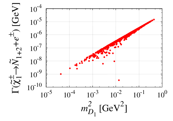
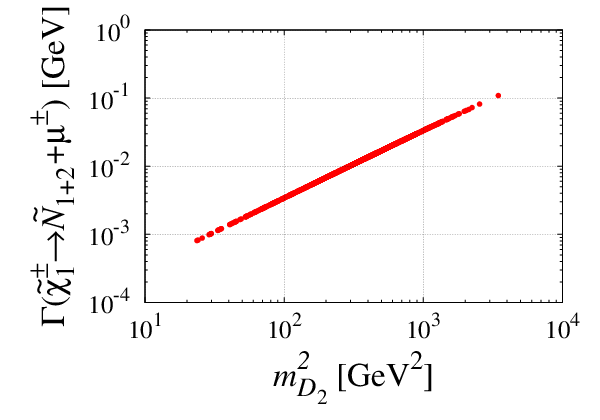
For the case , Fig. 2 shows the correlation of the decay width of the lightest chargino to the lightest pair of quasi-degenerate CP conjugated sneutrinos ( and ) and a charged lepton with respect to the corresponding parameter . We have checked that this correlation also holds for the chargino decay width , which involves the second lightest pair of quasi-degenerate CP conjugated sneutrinos ( and ). This behaviour is as expected from the analytical approximation in eq. (40). Note, however, that the correlation of the widths involving the electron with respect are not as clean than the others. This is due to the constraint on the neutrino reactor angle imposed by neutrino data, which requires to be much smaller than and . Comparing the size of these calculated widths to typical widths for final states and one finds that branching ratios into muon and tau final states can be sizeable, whereas the width to final state is expected to be too small to be measurable.
 |
 |
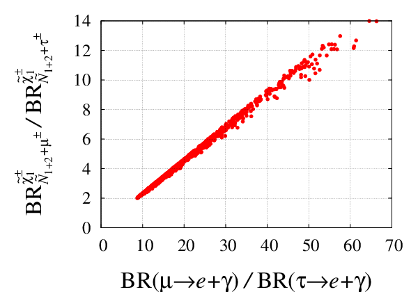
We note in passing that the product of the decay widths of the lightest chargino to one the two lightest pairs of quasi-degenerate CP conjugated sneutrinos and a charged lepton times the same width but to the charged lepton are correlated with the low energy LFV process . Again, the correlation involving the electron in the final state is less strong than the ones involving only and because of the relative smallness of the parameter imposed by the experimental upper bound on the neutrino reactor angle. Since the absolute widths, however, will not be measurable at the LHC, more interesting phenomenologically are ratios of partial widths, i.e. ratios of branching ratios.
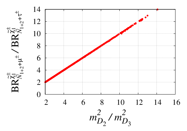
Fig. 3 shows ratios of branching ratios as a function of (left panel) and (right panel). Again, the same correlations can be found for . A measurement of both, chargino decays and LFV lepton decays, would therefore constitute a consistency check of the scenario we discuss. Note, however, that the expected branching ratio for is quite small (at most ) compared to current experimental sensitivities.
 |
 |
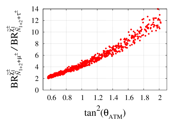
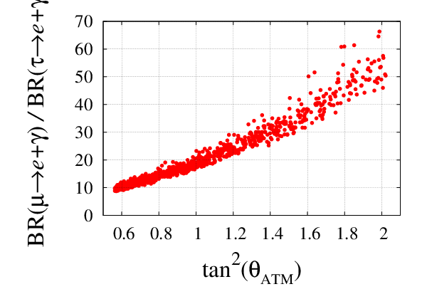
Left panel in Fig. 4 shows the correlation of the ratio of branching ratios of the lightest chargino decaying to the lightest sneutrino pair and divided by its decay to the lightest sneutrino pair and as a function of the atmospheric neutrino mixing angle. Recall that these data points have parameters chosen such that the atmospheric scale is generated by tree-level physics. The correlation exists for the lightest and for the next-to-lightest pair of singlet sneutrinos, if kinematically accessible. Right panel in Fig. 4 shows the correlation of the ratio of divided by as a function of the atmospheric neutrino mixing angle. As can be seen from both panels in Fig. 4, the neutrino sector (the atmospheric mixing angle) is related to collider observables (the LFV decays of the lightest chargino to a singlet sneutrino and a lepton) as well as low energy LFV observables (the radiative decays of the charged leptons).
 |
 |
As in our model we have relatively light right handed neutrinos and sneutrinos with large Yukawa coupling we should check the contributions from these new particles to the muon . We have calculated the new contributions to and verified that our numerical points - once they pass the cuts from - also pass the experimental constraint from [35].
Finally we would like to comment on the case , i.e. the parameters giving the dominant contribution to the neutrino mass matrix and thus to the lightest chargino LFV decays. We have scanned the parameter space of the model for such solutions and, as expected the decays of the charginos to singlet sneutrinos plus a lepton correlate with instead of in this extreme. However, in all points we have found the absolute widths for the final states plus a charged lepton are much smaller than in the case discussed above (at most of the order of GeV). One expects therefore that the corresponding branching ratios are too small to be measured at LHC.
5 Summary
The minimal supersymmetric inverse seesaw model (MSISM) with only one pair of singlet superfields can explain all existing neutrino oscillation data. We have calculated the neutrino mass matrix at 1-loop order and discussed the constraints on model parameters due to the experimentally measured leptonic mixing angles and neutrino masses.
Since in the MSISM one expects the new singlet fields to exist at a mass scale below (approximately) TeV, additional phenomenology is expected to show up in experiments searching for lepton flavour violation, such as , and possibly at the LHC. Absolute values of branching ratios can not be predicted, but the minimal model relates the observed atmospheric angle to some specific ratios of branching ratios. A measurement of these ratios can therefore potentially serve as a test of our minimal model.
For the LHC we have concentrated in our discussion on the case that one of the singlet scalar fields, a mixture of the scalar neutrino and the scalar singlet , is the lightest supersymmetric particle. This assumption is motivated by the observation that this singlet could be the CDM. Charginos can then decay to charged leptons plus singlet sneutrinos. A measurement of these decays and low energy lepton flavour violating lepton decays, such as and would provide an interesting test of the minimal supersymmetric inverse seesaw model.
Acknowledgments
This work was partially supported by FCT through the projects CFTP-FCT UNIT 777 and CERN/FP/83503/2008, which are partially funded through POCTI (FEDER), and by the Marie Curie RTN MRT-CT-2006-035505. M.H. is supported by the Spanish grant FPA2008-00319/FPA. A. V. M. is supported by Fundação para a Ciência e a Tecnologia under the grant SFRH/BPD/30450/2006.
Appendix A Higgs-heavy neutrino loop
Here we consider the 1-loop contributions to the neutrino mass matrix which are mediated through the Higgs-heavy neutrino loops. For their calculation, the required Lagrangian is given by
| (A.1) |
where denotes the unitary mixing matrix, which diagonalizes the mass matrix of the neutral fermion fields of eq. (4), . We note that only the contribution of the two heavy neutrinos is significant, and thus in (A.1) , , denotes the two heavy neutrinos which are a mixture of the fermionic states and . Contributions of light neutrinos in the loop are negligible, since the corresponding mixing elements , , are tiny. The neutral component of the up-type Higgs doublet can be expressed in terms of mass eigenstates as follows [32]
| (A.2) |
where are the two CP-even scalar fields, with and the corresponding mixing angle , is the CP-odd scalar field, while is the Goldstone field, with . From the calculation of the self-energy functions of these contributions we obtain
| (A.3) | |||||
| (A.4) |
where we have introduced the shorthand notations and , to sum up the various Higgs boson contributions. In eqs. (A.3)-(A.4), the standard 2-point loop integrals and , when evaluated at zero momentum (), can be written as
| (A.5) | |||||
| (A.6) |
We see from eqs. (A.3)-(A.4) that the flavor structure is determined by the product of the neutrino Yukawa couplings (in the flavor basis), and has therefore the same structure as the tree-level contribution, see eq. (5). As a result, only the 33-element in and receive non-vanishing contributions. Thus, by including only the Higgs-heavy neutrino loop contributions still two of the light neutrinos remain massless.
Appendix B LFV lepton decays
Here we summarize the formulas for the calculation of the two-body LFV lepton decay rates in the MSISM with only one generation of singlet superfields. The formulas are derived from the superpotential in eq. (2) and the soft SUSY breaking Lagrangian in eq. (3). In the context of the SUSY inverse seesaw mechanism with three generation of singlet superfields and mSugra boundary conditions see Ref. [29].
The gauge invariant amplitudes of the decays , , can be defined as [33]
| (B.1) |
In the calculation of the left and right amplitudes, , we neglected terms proportional to the small lepton mass . The heavy lepton contributions give rise to the right amplitude as [33, 34]
| (B.2) |
with . Note that the loop function in eq. (B.2) coincides with eq. (68) of [33], and differs by a constant, , from eq. (B.2) of Ref. [34]. For decays this constant does not contibute, due to the unitarity of the coupling matrices, but for the main contribution for light neutrinos comes precisely from this constant and therefore the correct loop function for both cases is eq. (B.2). The sneutrino-chargino loop contributions to the right amplitude read
| (B.3) | |||||
with and the couplings defined in eq. (37). The sneutrino-chargino loop contributions to the left amplitude are obtained from the right ones by interchanging the left and right chiral couplings, i.e. . With the definition of the amplitude in eq. (B.1), the corresponding decay widths are given by
| (B.4) |
with and where again in the kinematics we have neglected the terms proportional to the small lepton mass .
Appendix C Muon anomalous magnetic moment
The formulas for the muon anomalous magnetic moment can be derived from those in the previous section. Defining, as usual,
| (C.1) |
we have from eq. (B.1)
| (C.2) |
where and are defined, for our model, in eq. (B.2) and eq. (B.3). The sum in eq. (B.2) should run only over the heavy neutral leptons, as the light neutrino contribution is alreday included in the Standard Model. We have checked that our formulas reproduced the PDG [35] value for the sum of the and diagrams, at 1-loop order in the Standard Model.
References
- [1] Super-Kamiokande collaboration, Y. Fukuda et al., Phys. Rev. Lett. 81, 1562 (1998); Q. R. Ahmad et al. [SNO Collaboration], Phys. Rev. Lett. 89, 011301 (2002); K. Eguchi et al. [KamLAND Collaboration], Phys. Rev. Lett. 90, 021802 (2003).
- [2] For a review of neutrino oscillation data, see: M. Maltoni, T. Schwetz, M. A. Tortola and J. W. F. Valle, New J. Phys. 6, 122 (2004); an updated analysis has been published recently in: T. Schwetz, M. Tortola and J. W. F. Valle, New J. Phys. 10, 113011 (2008) [arXiv:0808.2016 [hep-ph]] where many additional experimental references can also be found.
- [3] D. N. Spergel et al. [WMAP Collaboration], Astrophys. J. Suppl. 148, 175 (2003) [arXiv:astro-ph/0302209].
- [4] E. Komatsu et al. [WMAP Collaboration], Astrophys. J. Suppl. 180, 330 (2009) [arXiv:0803.0547 [astro-ph]].
- [5] M. Tegmark et al. [SDSS Collaboration], Phys. Rev. D 74, 123507 (2006) [arXiv:astro-ph/0608632].
- [6] R. N. Mohapatra and J. W. F. Valle, Phys. Rev. D 34, 1642 (1986).
- [7] C. Arina, F. Bazzocchi, N. Fornengo, J. C. Romao and J. W. F. Valle, Phys. Rev. Lett. 101, 161802 (2008) [arXiv:0806.3225 [hep-ph]].
- [8] S. Weinberg, Phys. Rev. Lett. 43, 1566 (1979); S. Weinberg, Phys. Rev. D 22, 1694 (1980).
- [9] E. Ma, Phys. Rev. Lett. 81, 1171 (1998) [arXiv:hep-ph/9805219].
- [10] P. Minkowski, Phys. Lett. B 67, 421 (1977).
- [11] T. Yanagida, in Proc. of the Workshop on the Baryon Number of the Universe and Unified Theories, National Laboratory for High Energy Physics (KEK), February 13-14, 1979, edited by O. Sawada and A. Sugamoto (National Laboratory for High Energy Physics, Tsukuba, Japan, 1979); M Gell-Mann, P Ramond, R. Slansky, in Supergravity, edited by P. van Niewenhuizen, and D. Freedman (North Holland Publ. Co., Amsterdam, 1979); R.N. Mohapatra and G. Senjanovic, Phys. Rev. Lett. 44, 912 (1980); J. Schechter and J. W. F. Valle, Phys. Rev. D 22, 2227 (1980).
- [12] T. P. Cheng and L. F. Li, Phys. Rev. D 22, 2860 (1980).
- [13] A. Zee, Phys. Lett. B93, 389 (1980).
- [14] K. S. Babu, Phys. Lett. B 203, 132 (1988). A. Zee, Nucl. Phys. B 264, 99 (1986).
- [15] G. ’t Hooft, Lecture given at Cargese Summer Inst., Cargese, France, Aug 26 - Sep 8, 1979.
- [16] M. Malinsky, T. Ohlsson, Z. z. Xing and H. Zhang, Phys. Lett. B 679, 242 (2009) [arXiv:0905.2889 [hep-ph]].
- [17] M. Hirsch, H. V. Klapdor-Kleingrothaus and S. G. Kovalenko, Phys. Lett. B 398, 311 (1997) [arXiv:hep-ph/9701253].
- [18] M. Hirsch, M. A. Diaz, W. Porod, J. C. Romao and J. W. F. Valle, Phys. Rev. D 62 (2000) 113008 [Erratum-ibid. D 65 (2002) 119901] [arXiv:hep-ph/0004115].
- [19] G. Jungman, M. Kamionkowski and K. Griest, Phys. Rept. 267, 195 (1996) [arXiv:hep-ph/9506380].
- [20] G. Bertone, D. Hooper and J. Silk, Phys. Rept. 405, 279 (2005) [arXiv:hep-ph/0404175].
- [21] T. Falk, K. A. Olive and M. Srednicki, Phys. Lett. B 339, 248 (1994) [arXiv:hep-ph/9409270].
- [22] T. Asaka, K. Ishiwata and T. Moroi, Phys. Rev. D 73, 051301 (2006); T. Asaka, K. Ishiwata and T. Moroi, Phys. Rev. D 75, 065001 (2007) [arXiv:hep-ph/0612211].
- [23] S. Gopalakrishna, A. de Gouvea and W. Porod, JCAP 0605, 005 (2006) [arXiv:hep-ph/0602027].
- [24] N. Arkani-Hamed, L. J. Hall, H. Murayama, D. Tucker-Smith and N. Weiner, Phys. Rev. D 64, 115011 (2001) [arXiv:hep-ph/0006312].
- [25] C. Arina and N. Fornengo, JHEP 0711, 029 (2007) [arXiv:0709.4477 [hep-ph]].
- [26] F. Deppisch and A. Pilaftsis, JHEP 0810, 080 (2008) [arXiv:0808.0490 [hep-ph]].
- [27] H. S. Lee, K. T. Matchev and S. Nasri, Phys. Rev. D 76, 041302 (2007) [arXiv:hep-ph/0702223].
- [28] D. G. Cerdeno and O. Seto, JCAP 0908, 032 (2009) [arXiv:0903.4677 [hep-ph]]; D. G. Cerdeno, C. Munoz and O. Seto, Phys. Rev. D 79, 023510 (2009) [arXiv:0807.3029 [hep-ph]].
- [29] F. Deppisch and J. W. F. Valle, Phys. Rev. D 72, 036001 (2005) [arXiv:hep-ph/0406040].
- [30] A. Dedes, H. E. Haber and J. Rosiek, JHEP 0711, 059 (2007) [arXiv:0707.3718 [hep-ph]].
- [31] P. F. Harrison, D. H. Perkins and W. G. Scott, Phys. Lett. B 530, 167 (2002) [arXiv:hep-ph/0202074].
- [32] J. F. Gunion and H. E. Haber, Nucl. Phys. B 272, 1 (1986) [Erratum-ibid. B 402, 567 (1993)].
- [33] L. Lavoura, Eur. Phys. J. C 29, 191 (2003) [arXiv:hep-ph/0302221].
- [34] A. Ilakovac and A. Pilaftsis, Nucl. Phys. B 437, 491 (1995) [arXiv:hep-ph/9403398].
- [35] C. Amsler et al. [Particle Data Group], Phys. Lett. B 667, 1 (2008).