Proper heavy-quark potential from a spectral decomposition of the thermal Wilson loop
Abstract:
We propose a non-perturbative and gauge invariant derivation of the static potential between a heavy-quark () and an anti-quark () at finite temperature. This proper potential is defined through the spectral function (SPF) of the thermal Wilson loop and can be shown to satisfy the Schrödinger equation for the heavy pair in the thermal medium. In general, the proper potential has a real and an imaginary part, corresponding to the peak position and width of the SPF. The validity of using a Schrödinger equation for heavy can also be checked from the structure of the SPF. To test this idea, quenched QCD simulations on anisotropic lattices (, ) are performed. The real part of the proper potential below the deconfinement temperature () exhibits the well known Coulombic and confining behavior. At () we find that it coincides with the Debye screened potential obtained from Polyakov-line correlations in the color-singlet channel under Coulomb gauge fixing. The physical meaning of the spectral structure of the thermal Wilson loop and the use of the maximum entropy method (MEM) to extract the real and imaginary part of the proper potential are also discussed.
July 26-31, 2009
Peking University, Beijing, China
1 Introduction
Heavy quarkonium at finite temperature is a both intriguing and challenging subject. In particular, its in-medium behavior has been proposed to be a prime signal for the creation of the quark-gluon plasma (QGP), expected above the critical temperature of the deconfinement transition [1]. Moreover, the advent of RHIC has made it possible to access the QGP in the laboratory [2] and a partial suppression of charmonium has been experimentally confirmed [3].
In the meantime, theoretical understanding has also progressed significantly. Originally, a non-relativistic Schrödinger equation with screened Coulomb potential was considered for the heavy pair above [1]. Later on, more sophisticated potentials were adopted, such as the color-singlet free-energy of a static pair and its variants [4]. A main drawback of these approaches is that there is no firm theoretical foundation to use such potentials within the Schrödinger equation of a heavy pair in a hot environment.11 1 This is in contrast to the situation at zero temperature in which a systematic way to derive the potential to be used in the Schrödinger equation has been formulated in the framework of non-relativistic QCD [5]. A more direct approach to heavy quarkonium at finite temperature is to extract the spectral function (SPF) from lattice QCD simulations with the help of the maximum entropy method (MEM) [6]. An unexpected feature found subsequently was that charmonium may survive even above the deconfinement transition up to about 2 [7, 8]. However, a transparent understanding of this result has not been obtained so far.
In light of these circumstances it is imperative to establish a solid connection between the Schrödinger approach and the spectral function approach, based on a proper definition of the in-medium potential. A possible way to reach this goal was initially proposed in [9]; the proper potential to be used in the in-medium Schrödinger equation was defined from the late-time () behavior of the forward correlator of a heavy pair separated by distance (). It was shown by using hard thermal resummation (HTL) techniques at high that the potential has both a real and an imaginary part. The purpose of the present article is to develop this idea further by introducing a spectral decomposition of (or equivalently the thermal Wilson loop) and to explore the non-perturbative derivation of the real and imaginary part of the proper potential on the basis of lattice QCD simulations. If this program turns out to be successful, a true physical understanding of the heavy-quark bound state in the QGP can possibly be obtained.
2 Formulation
2.1 Spectral function for a static pair
We start with the operator defined as , where and . The Wilson-line operator is chosen to connect the points and by a straight space-like path . An arbitrary Dirac matrix is denoted by , e.g. in the vector channel and in the pseudoscalar channel. Let us introduce the forward correlation function of the pair,
| (1) |
In a fully dynamic setting, heavy quarks can propagate in time, hence the relative distance between and will change accordingly. On the other hand, if we consider the infinite mass case (), the spatial separation reduces to an external parameter. The spectral function associated with Eq.(1) reads
| (2) |
where , is the Fourier transform of , and is the full partition function of the system with gluons, light quarks and heavy quarks. Eq.(2) is antisymmetric in due to the bosonic character of the operator .
We now consider heavy quarks with nearly infinite mass , so that they cannot move spatially and their relative distance stays fixed. The spectral function can thus be decomposed into the sum of the three contributions, depending on the intermediate states given below (”light” implies light quarks and gluons):
| I | II | III | |
|---|---|---|---|
| light | or | ||
| light | or |
Since we are interested in the interaction between and with a spatial separation at the same point in time, only the contributions I and II are relevant for our purpose. Moreover, I and II are simply related with each other by , due to the anti-symmetric nature of the SPF. Without loss of generality, it is therefore sufficient to focus on the contribution I. By taking into account the fact that , we obtain
| (3) |
where is the partition function without the heavy quarks, and belong to the case I in the above Table. Also, we have defined , and . Note that is the -dependent energy of a pair measured from the total rest mass , while is -independent since no heavy quarks are present in the state . Note that they are both -independent by definition.
The spectral structure of contains all the information of the interaction between the heavy quarks in the hot medium. To see its connection to the Schrödinger equation for the heavy quark system, let us start with the following relation obtained from the definitions of and :
| (4) |
If has a distinct Breit-Wigner peak at with a half-width , Eq.(4) reduces to the Schrödinger equation,
| (5) | |||||
with being the proper heavy-quark potential at finite temperature. On the other hand, if there are no well-defined peaks in , description of the system in terms of the potential is not justified. Note that the existence of was first pointed out in [9] in which the late time behavior of was calculated in hard thermal loop resummation at high .
2.2 Thermal Wilson loop and its spectral decomposition
To evaluate the spectral function defined in Eq.(3) in non-perturbative lattice QCD simulations, we consider the imaginary-time correlator . Since the heavy quarks are assumed not to propagate in the spatial directions, their imaginary time propagator has the form with being written in terms of temporal Wilson-lines. For the full correlator we obtain
| (6) | |||||
| (7) | |||||
| (8) |
where the numerical coefficients are defined as e.g. with being the projection operator onto the upper and lower components of the Dirac spinor. are the Wilson-loops at finite temperature with different topological structure (loop, staple and handle) as shown in Fig.1.
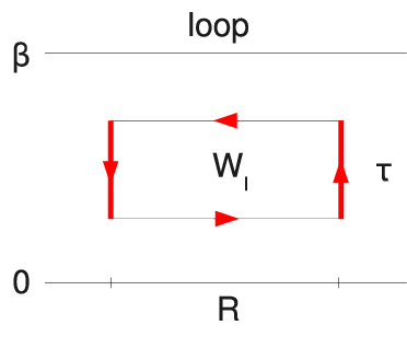


From their -dependence and particle content in the intermediate state, it is easy to see that loop, staple and handle correspond to the case I, case II and case III respectively. Namely the loop contribution given in Eq.(6) has the spectral decomposition,
| (9) |
Thus we arrive at the following formula relating the thermal Wilson loop with the spectral function,
| (10) |
Note that this relation is well-defined in the limit .
Lattice QCD simulations of the left hand side of Eq.(10) for different values of and allow a non-perturbative determination of the spectral function through the inverse Laplace transform, e.g. by using the MEM. The peak position and its width can consequently be translated into the real and imaginary part of the proper potential.
3 Quenched QCD results at low and high
To study the feasibility of the method proposed above, we perform quenched lattice QCD simulations using the plaquette gauge action with on an anisotropic lattice. The physical lattice spacing and anisotropy are the same with the first reference in [7], . We adopt the fixed scale method [11] where one varies to change the temperature. An advantage of this method is that the lattice spacing is the same for all temperatures so that the potentials for different temperatures can be directly compared without any adjustment. The thermal Wilson loop is calculated as a function of and . We report here only the results at the lowest temperature () and the highest temperature () using () gauge configurations respectively.


Shown in the left panel of Fig.2 is the on-axis thermal Wilson loop as a function of for different values of in the low-temperature confinement phase (). By definition, it is not symmetric under the reflection . In the small region, an effect from + excited gluons can be seen, which is similar to the case of the standard hadronic correlation functions. In the intermediate region, we find a single exponential behavior, which suggests the existence of a distinct peak of vanishing width in the spectral function. The position of the peak is nothing but the real part of the proper potential . We make a single exponential fit of for each in the interval (). The result is plotted as a function of in the right panel of Fig.2 with filled squares. Error bars estimated by a fit for several slightly shifted or contracted fitting regions reflect both the statistical and systematic uncertainties. The data can be fitted well by a Coulomb + linear form with an effective string tension as indicated by the gray line. This is smaller than the known value at , possibly due to the thermal fluctuations of the confining string. We emphasize here that (i) the thermal Wilson loop is directly linked to the Schrödinger equation as we have discussed and (ii) one can obtain not only the real part but also the imaginary part of the proper potential from the thermal Wilson loop by using e.g. MEM. Analysis of the present lattice data in the whole range of by using MEM is currently under way.


Shown in the left panel of Fig.3 is the thermal Wilson loop in the high temperature deconfinement phase (). In this case, we find three characteristic features: For , some evidence for excited states can be seen. For , there appears an approximate single exponential behavior which indicates a well-defined peak in the spectral function. For , the thermal Wilson loop increases as increases, which indicates that the spectral function has some structure for negative although the spectral strength is extremely small. This may be interpreted as the effect of thermal gluons with energy ; they can compensate a deficit of the external energy to match the energy conservation, or equivalently , so that a can appear in the intermediate state. A triple exponential fit is deployed, designed to give stable results in the presence of non single-exponential behavior coming from the end regions of the interval. The fit results of for each in the interval () leads to the plot in the right panel of Fig.3. It shows a Coulombic behavior at short distances, while the potential seems to be Debye screened at long distances. For comparison, we measure the color-singlet free energy on the same lattice from the Polyakov line correlations in the color-singlet channel under Coulomb gauge fixing: . The results are shown by the open circles. Although and have no direct theoretical connection, they coincide within the error margins devoid of any adjustments. An analysis of the present lattice data over the whole range of by using MEM is currently under way to extract the complete spectral structure of . This will enable us to extract and also to judge the validity of the potential picture at high .
4 Summary and concluding remarks
We proposed a non-perturbative and gauge invariant approach to connect the Schödinger equation description of a heavy pair in terms of a static potential with the spectral function of the thermal Wilson loop obtained from Lattice QCD. It was shown that if the spectral structure is well defined for a set of temperatures and separation distances , the peak position and width correspond to the real and imaginary part of the proper potential respectively. A first determination of the real part of the proper potential from quenched lattice QCD simulations () was presented for and . It showed that although no apparent connection between the real part of the proper potential and the color-singlet free-energy potential exist, their values above coincide within the error bars. We are currently analyzing the thermal Wilson loop data for , using MEM to determine the full spectral structure in an attempt to reconstruct not only the real but also the imaginary part, especially above the phase transition. In the case of infinitely heavy quarks, the only contribution to such an imaginary part at high comes from the scattering of light medium particles, i.e. Landau damping [9, 10]. The non-perturbative determination of and for is particularly important in relation to the fate of charmonium above .
Two directions for future research are thus in order: (i) we need to include the effects of light fermions in the medium by utilizing full QCD configurations, and (ii) the approach has to be extended to finite masses. As for (ii), a similar strategy as for , where the spatial fluctuations of the heavy quarks are incorporated by appropriate insertion of handles in the temporal Wilson lines [12] might be a first starting point.
We thank Yuu Maezawa and the members of the WHOT-QCD Collaboration for useful discussions. This research was supported in part by the Grant-in-Aid of MEXT (Nos. 18540253) and by Grant-in-Aid for Scientific Research on Innovative Areas (No. 2004: 20105003).
References
- [1]
T. Matsui and H. Satz,
Phys. Lett. B 178, 416 (1986).
T. Hashimoto, K. Hirose, T. Kanki and O. Miyamura, Phys. Rev. Lett. 57, 2123 (1986). - [2] Reviewd in K. Yagi, T. Hatsuda and Y. Miake, Quark-Gluon Plasma, (Cambridge Univ. Press, Cambridge, 2005).
- [3] Reviewed in R. Rapp and H. van Hees, arXiv:0903.1096 [hep-ph].
- [4] Reviewed in H. Satz, arXiv:0812.3829 [hep-ph].
- [5] N. Brambilla, A. Pineda, J. Soto and A. Vairo, Rev. Mod. Phys. 77, 1423 (2005) [arXiv:hep-ph/0410047].
- [6] M. Asakawa, T. Hatsuda and Y. Nakahara, Prog. Part. Nucl. Phys. 46, 459 (2001) [arXiv:hep-lat/0011040].
- [7] M. Asakawa and T. Hatsuda, Phys. Rev. Lett. 92, 012001 (2004) [arXiv:hep-lat/0308034]. S. Datta, F. Karsch, P. Petreczky and I. Wetzorke, Phys. Rev. D 69, 094507 (2004) [arXiv:hep-lat/0312037]. T. Umeda, K. Nomura and H. Matsufuru, Eur. Phys. J. C 39S1, 9 (2005) [arXiv:hep-lat/0211003]. A. Jakovac, P. Petreczky, K. Petrov and A. Velytsky, Phys. Rev. D 75, 014506 (2007) [arXiv:hep-lat/0611017]. G. Aarts, C. Allton, M. B. Oktay, M. Peardon and J. I. Skullerud, Phys. Rev. D 76, 094513 (2007) [arXiv:0705.2198 [hep-lat]].
- [8] Reviewed in C. DeTar and U. M. Heller, “QCD Thermodynamics from the Lattice,” Eur. Phys. J. A 41, 405 (2009) [arXiv:0905.2949 [hep-lat]].
- [9] M. Laine, O. Philipsen, P. Romatschke and M. Tassler, JHEP 0703, 054 (2007) [arXiv:hep-ph/0611300]. Y. Burnier, M. Laine and M. Vepsalainen, JHEP 0801, 043 (2008) [arXiv:0711.1743 [hep-ph]].
- [10] A. Beraudo, J. P. Blaizot and C. Ratti, Nucl. Phys. A 806, 312 (2008) [arXiv:0712.4394 [nucl-th]].
- [11] T. Umeda et al. (WHOT-QCD Collabolation), Phys. Rev. D 79, 051501 (2009) [arXiv:0809.2842 [hep-lat]]. Y. Maezawa et al. (WHOT-QCD Collaboration), in these proceedings.
- [12] Y. Koma, M. Koma and H. Wittig, Phys. Rev. Lett. 97, 122003 (2006) [arXiv:hep-lat/0607009].