UCB-PTH-09/31
A Finely-Predicted Higgs Boson Mass
from
A Finely-Tuned Weak Scale
Lawrence J. Hall and Yasunori Nomura
Berkeley Center for Theoretical Physics, Department of Physics,
and Theoretical Physics Group, Lawrence Berkeley National Laboratory,
University of California, Berkeley, CA 94720, USA
and
Institute for the Physics and Mathematics of the Universe,
University of Tokyo, Kashiwa 277-8568, Japan
If supersymmetry is broken directly to the Standard Model at energies not very far from the unified scale, the Higgs boson mass lies in the range . The end points of this range are tightly determined. Theories with the Higgs boson dominantly in a single supermultiplet predict a mass at the upper edge, , with the uncertainty dominated by the experimental errors on the top quark mass and the QCD coupling. This edge prediction is remarkably insensitive to the supersymmetry breaking scale and to supersymmetric threshold corrections so that, in a wide class of theories, the theoretical uncertainties are at the level of . A reduction in the uncertainties from the top quark mass and QCD coupling to the level of may be possible at future colliders, increasing the accuracy of the confrontation with theory from to . Verification of this prediction would provide strong evidence for supersymmetry, broken at a very high scale of , and also for a Higgs boson that is elementary up to this high scale, implying fine-tuning of the Higgs mass parameter by orders of magnitude. Currently, the only known explanation for such fine-tuning is the multiverse.
1 Overview
The Standard Model (SM), taken to include neutrino masses, has reigned supreme for over three decades. Despite strenuous efforts, at lepton and hadron colliders and from astrophysical observation, there is no hard evidence to contradict the Standard Model together with General Relativity (SM GR) as the entire effective theory of nature up to extraordinarily high energies.
Over these decades, there have been many theoretical arguments for physics beyond the SM, with supersymmetry figuring very prominently and having two very different theoretical motivations:
- •
String theory contains a quantum theory of gravity, and is the leading candidate theory for the unification of all the fundamental interactions. It requires supersymmetry in a spacetime with extra spatial dimensions, but leaves open the question of the size of supersymmetry breaking, which experiment allows to be anywhere in the range of the weak scale to the string scale.
- •
If supersymmetry breaking in the SM sector, , is of order the weak scale, , then the smallness of the weak scale relative to the Planck scale can be naturally understood. In particular, a fine-tuning of the Higgs mass parameter to thirty orders of magnitude is avoided, and an elegant radiative mechanism for breaking of electroweak symmetry emerges.
Taken together, the theoretical motivation for supersymmetry is high, with the hope that superpartners are in reach of current hadron colliders.
Have experiments given any hint, positive or negative, on whether supersymmetric particles are at the weak scale?
- •
Since the first experiments at LEP, it has become clear that the three SM gauge couplings unify more precisely if the theory is supersymmetric, with of order . Threshold corrections at the unified scale required for unification are fully an order of magnitude smaller with weak scale supersymmetry than without. These corrections can arise from a mild non-degeneracy of one or two small multiplets at the unified scale with supersymmetry, but more multiplets or larger splittings are required without supersymmetry.
- •
The lightest weak scale superpartner can be stable, providing a Weakly Interacting Massive Particle (WIMP) candidate for Dark Matter (DM). It is intriguing that WIMPs, particles with order unity dimensionless couplings and order dimensionful couplings, lead to the observed abundance of DM, at least within a few orders of magnitude.
- •
A light Higgs boson, as expected in the simplest theories with weak scale supersymmetry, has not been found. These theories now require a tuning of parameters, typically at the percent level, to reproduce the observed weak gauge boson masses.
In the first years after LEP, the first two items above provided a strong motivation for taking supersymmetry as the leading candidate for understanding the weak scale. However, the absence of a light Higgs boson is certainly a problem for simple natural theories. Furthermore, together with experimental bounds on superpartner masses, it pushes these theories into regions where the superpartner WIMP candidates are also unnatural. This unease with weak scale supersymmetry is compounded by the lack of any signals of new flavor or violation beyond the SM, such as , and by cosmological issues, such as the gravitino problem. Over the years there were many opportunities for supersymmetry to become manifest, leaving us today with many reasons to question weak scale supersymmetry. The single remaining success is gauge coupling unification, and while this is certainly significant, one wonders whether a decrease in the unified threshold corrections by an order of magnitude might be an unfortunate accident. Even without supersymmetry, unification can occur, either by enhancing these threshold corrections or by certain matter surviving below the unified scale. Indeed, the evolution of the gauge couplings in the SM shows evidence for unification [1], as shown in Figure 1, and precision unification requires only a small perturbation to this picture.

What, then, is the origin of the weak scale? It has been suggested that the weak scale may result from anthropic, or environmental, selection [2]. In particular, if the Higgs mass parameter scans effectively in the multiverse, but not the Yukawa couplings, then the requirement of the stability of some complex nuclei requires that the weak scale be no more than a factor two larger than we measure [2, 3]. In this picture, most universes have weak interactions broken at a very high scale or by QCD dynamics, but they contain no complex nuclei and consequently no observers. This view is often dismissed on the grounds that no evidence can be obtained for the multiverse, but this is incorrect. For example, consider Split Supersymmetry [4]: the weak scale is determined by environmental selection and supersymmetry is broken at some high scale , but the fermionic superpartners are taken at the TeV scale to account for DM. In this theory, collider measurements of the fermionic superpartner interactions could lead to a convincing determination of and demonstration that the Higgs field is elementary at the scale . This would imply a fine-tuning in the Higgs mass parameter of in , which could be as large as . Fine-tuning that has no symmetry explanation is key evidence of the multiverse.
While environmental selection in the multiverse is speculative, we think it is the leading explanation for the order of magnitude of the cosmological dark energy [5] providing the only understanding for orders of magnitude of fine-tuning. Indeed, we are greatly motivated by this result. Dark energy does not need any addition to the SM minimally coupled to gravity, and the prediction for the equation of state, , agrees well with current data, [6]. Of course, this requires a huge number of vacua, a landscape, that allows for sufficiently fine scanning of the cosmological constant, and it brings us back to the first theoretical motivation for supersymmetry, string theory, which is believed to have a landscape of sufficient size to allow the selection of both the cosmological constant and the weak scale [7].
In this paper we assume that the weak scale is determined by environmental selection. Where does that leave supersymmetry? While the motivation from fine-tuning is gone, the motivation from string theory is strengthened, since the landscape has its origin in string theory. In seeking observational evidence for supersymmetry, the two key questions are then
- •
What is ?
- •
Are there any non-SM particles near the weak scale?
We stress that, with the weak scale arising from environmental selection, we have lost the logical connection from naturalness between and , and hence the expectation of superpartners at the weak scale.
The argument that some non-SM particles must survive to the weak scale, becoming WIMPs to account for DM, is not correct. How is the strong problem to be solved? The small size of violation in the strong interaction must be understood from conventional symmetry arguments; environmental selection cannot explain the smallness of the QCD angle, , because there is no known catastrophic boundary involving . Indeed, string theory is expected to contain a QCD axion, and therefore the Peccei-Quinn solution to the strong problem [8]. This leads to the expectation that axions [9] are DM, with its density possibly determined by environmental requirements, removing any need for WIMP DM. Of course, there could be WIMP DM in addition to axion DM, but it is not necessary.
In this paper we therefore study the following simple framework: the supersymmetry breaking scale is very high, perhaps near the high energy cutoff of the field theory , above which a string description becomes a necessity. Below , the effective theory is SM GR. Experimentally this sounds like a “nightmare” scenario, since the LHC may discover only the Higgs boson, with no hint of any physics beyond the SM. This is, however, not true. We find that, although supersymmetry is broken at such high scales, a supersymmetric boundary condition on the Higgs quartic parameter is expected, leading to a narrow range for the Higgs boson mass of about . Discovering a Higgs boson in this mass range would certainly be interesting, but it would be far more significant if the Higgs boson mass is close to the upper edge of this range. This upper edge corresponds to the special situation that the Higgs boson resides dominantly in a single supermultiplet, and yields the prediction
| (1) |
Remarkably, the largest contribution to the uncertainty results from the experimental errors on the top quark mass and the QCD coupling, which can be improved by future experiments to . The scenario can therefore be tested to high precision.
It is important that the prediction of Eq. (1) does not depend sensitively on parameters that we cannot measure at low energies. In a large class of theories, with ranging over a few orders of magnitude and with a variety of superpartner spectra, the theoretical uncertainties are extremely small, about or less, reflecting both an infrared quasi-fixed point behavior of the Higgs quartic coupling and a reduced top Yukawa coupling at high energies. Since the uncertainties arising from our lack of knowledge of the underlying high energy theory are so small, a measurement of this special value for the Higgs boson mass would provide strong evidence for the framework.
In fact, the prediction of Eq. (1) survives even when the theory below is mildly extended beyond the SM. The conditions for such a precise prediction are that additional multiplets must make limited contributions to the beta functions of the SM gauge couplings, and that any new couplings to the Higgs boson must not be large.
A confirmation of the above Higgs mass prediction, together with the LHC finding no new physics beyond the SM, would provide significant evidence against our current paradigm and point to a very different picture of fundamental physics. In fact, the observation of this single number would have many implications:
- (i)
Supersymmetry would be “discovered,” but with superpartners somewhere near , rather than at the weak scale. The discovery of supersymmetry would point to string theory, but the large breaking scale would radically change string compactification phenomenology. All the ideas for new TeV physics—supersymmetry, technicolor, composite Higgs, and so on—would be replaced by the extension of the validity of the SM, perhaps augmented by a few small multiplets, up to very high energies.
- (ii)
Axions provide the only compelling solution to the strong problem, and hence axion DM would seem highly probable. As the axion decay constant is expected to be very high, a pressing question becomes why the universe is not overclosed by axions. This question has already been addressed: an environmental requirement on the density of DM may select the initial axion misalignment angle in our universe to be small [10]. WIMP DM, whether superpartners or not, would be unnecessary, although not excluded.
- (iii)
The apparent success of supersymmetric gauge coupling unification would be seen to be an accident, that misled much of the field for two decades. The evolution of gauge couplings would still point to unification, as shown for the case of the SM in Figure 1. The SM alone requires larger unified threshold corrections, and leads to a lower, more uncertain, unification scale, . Another possibility is that a few light multiplets additional to the SM lead to a precise unification, as in the case of a single vector-like lepton doublet near the weak scale.
- (iv)
Most important, there would be a huge fine-tuning in the Higgs boson mass parameter of orders of magnitude or more. The Higgs mass prediction would show that the Higgs boson is elementary up to very high energies, and there is no known symmetry mechanism that could tame the fine-tuning, given the high scale of supersymmetry breaking. This would provide strong evidence that the electroweak symmetry breaking scale results from environmental selection.
To avoid these conclusions, one must either assume that the success of the Higgs mass prediction at the GeV level is an accident, or come up with an alternative understanding of the large amount of fine-tuning.
In the final section of the paper, we argue that certain other values of the Higgs boson mass could also demonstrate both an elementary Higgs boson to high scales and an absence of supersymmetry beneath the high scale, again providing evidence for environmental selection in the multiverse.
2 A Supersymmetric Boundary Condition on
If the SM becomes supersymmetric at scale , then there is a boundary condition on the quartic Higgs coupling
| (2) |
where and are the and gauge couplings, and . The SM Higgs doublet is a combination of doublets of opposite hypercharge in the supersymmetric theory, described by a mixing angle . If is very large, does this boundary condition survive? For example, suppose supersymmetry is broken by the highest component VEV, , of a chiral superfield , so that . In general, the Kähler potential includes the higher dimension operator where is the Higgs superfield, so that the quartic coupling deviates from the supersymmetric boundary condition by an amount . With supersymmetry at the weak scale, , so this correction is negligible; but for high scale supersymmetry breaking, does this correction destroy any Higgs mass prediction?
Many parameters, including , are expected to vary in the multiverse. High scale supersymmetry results if the landscape distribution for increases sufficiently rapidly at large . For a given value of , we can determine whether a larger value is more probable by comparing whether the increase in probability from the distribution compensates for the more precise cancellation needed to keep below the environmental bound. We expect that a larger is more probable if, at the value of under consideration, the distribution grows more rapidly than quadratically. As continues to grow, the distribution may become milder than quadratic, so that in typical universes observers find . However, in this case the form of the distribution introduces a new mass scale. It seems more probable that the stronger peaking of the distribution persists all the way to near the cutoff , so that typical observers find close to . This apparently destroys the boundary condition for completely. We argue below, however, that even in this case the supersymmetric boundary condition may well persist.
The new physics around the cutoff is likely to be accompanied by the compact spatial manifold that results from string theory. How large do we expect this new scale to be? With near , it is reasonable to assume that it is not far from the scale of SM gauge coupling unification, . In this case the volume of the manifold is large, in units of the string scale, to account for the very large value of the Planck scale, . There are two ways that such a setup may act to preserve the supersymmetric boundary condition. First, the strength of supersymmetry breaking may not really reach . For small supersymmetry breaking, an increase in is unlikely to affect the dynamics at . However, as approaches , it may lead to a destabilization of the vacuum that yields the desired SM physics at low energy; may be prevented from reaching for an environmental reason. The second possibility is that supersymmetry breaking is maximal but, because it is now occurring in a higher dimensional manifold, it is no longer true that it leads to sizable . Below we discuss ways in which the spatial properties of supersymmetry breaking can suppress .
Supersymmetry breaking may either occur locally somewhere in the manifold, or it may be delocalized, as with Scherk-Schwarz or moduli breaking. Local breaking of supersymmetry may typically occur far from the localization of the SM matter and Higgs sector. In this case a non-local mediation mechanism is required and, given the large spatial separation, supersymmetry breaking in the SM Higgs sector is suppressed even if the local breaking of supersymmetry is maximal. The non-local transmission may be by loops of quanta propagating in the bulk, which may include SM gauge fields. The effects of tree-level transmissions are suppressed by the relevant volume factors; in particular, the gravity mediation contribution to is suppressed by . Once SM superpartners acquire mass, integrating them out gives loop threshold corrections to . These are computed in the next section and found to be small.
What if supersymmetry breaking is non-local? In this case is determined by , where () is an angle appearing in the compactification boundary conditions and is the size of the relevant extra dimension, which we take to be sufficiently larger than the cutoff scale for the classical spacetime picture to be valid. Ignoring gravity, any tree-level corrections to are suppressed by powers of . There are loop threshold corrections to from integrating out superpartners and Kaluza-Klein (KK) excitations of SM particles. The contributions from KK modes decouple if is small and, as mentioned, the contributions from superpartners are small. Even for , the contribution from KK modes is loop suppressed. The size of the gravity mediation contribution depends on the stabilization mechanism for the extra dimensions. The correction to , however, is suppressed by at least and typically much more.
Thus, even for maximal supersymmetry breaking, which likely leads to not far from , the supersymmetric boundary condition for may very well survive. Indeed, the boundary condition is expected to be destroyed only in the very specific situation that supersymmetry breaking and the SM Higgs sector have coincident locations in the extra dimensions, and the supersymmetry breaking is maximal, with hard up against the cutoff.
3 A Precise Prediction for the Higgs Boson Mass
A prediction for the Higgs boson mass results from a supersymmetric boundary condition on the Higgs quartic coupling at ; however, the uncertainties might be very large. Indeed, in the Minimal Supersymmetric Standard Model (MSSM) one-loop threshold corrections from top squark loops at lead to corrections to the Higgs boson mass as large as . For weak scale supersymmetry, collider measurements of superpartner properties could determine the threshold corrections, but this is clearly not possible for supersymmetry breaking at unified scales. In this section we show that this naive expectation, of large uncertainties to the Higgs mass prediction from threshold corrections, is completely incorrect; rather, the largest uncertainties come from the experimental uncertainties on the top quark mass, , and the QCD coupling, , which are already small and can be reduced by future precise measurements.
In section 3.1, we compute the Higgs boson mass when the theory below is the SM, paying attention to possible threshold corrections from the scale . In section 3.2, we explore the sensitivity of the prediction to additional states with SM gauge interactions far below , and in section 3.3 we discuss the relation to other work.
All figures and analytical results are obtained using two-loop renormalization group (RG) scaling of all couplings from to the weak scale, together with one-loop threshold corrections at the weak scale, including the one-loop effective potential for the Higgs field. In addition, we include the two- and three-loop QCD threshold corrections in converting the top-quark pole mass to the top Yukawa coupling, since they are anomalously large. Experimental values of [11] and [12] are used.
3.1 SM below
In a general supersymmetric model, the SM Higgs doublet may be a combination of supersymmetric Higgs doublets having opposite hypercharge so that, before including threshold corrections, the boundary condition on the quartic coupling is given by Eq. (2). The resulting prediction is actually a correlation between the Higgs boson mass and the parameter , as shown by the solid red curve in Figure 2.

Remarkably, even as varies over all possible values, the Higgs mass lies in a narrow, high-scale supersymmetry, window of . Furthermore, for large values of the Higgs mass rapidly asymptotes to , shown by the blue line, reaching of this asymptote at .
As discussed in the next section, in many simple supersymmetric theories the parameter is too large to be relevant or even does not exist, so that from now on we study the boundary condition
| (3) |
where includes all threshold corrections from the scale , and is expected to be if is chosen close to the superparticle masses. The effect of finite can be included as a contribution to
| (4) |
The Higgs mass prediction following from Eq. (3) takes the form , with both an explicit dependence on and an implicit one via . Since is an arbitrary matching scale, is independent of : the explicit and implicit dependences cancel. However, does depend on the spectrum of superpartners via the expression for , with a typical sensitivity that can be estimated by studying the explicit dependence of on , or equivalently on . As shown below, for a wide range of and , these sensitivities of are extremely mild.
In Figure 3, we show the numerical solution for the running coupling as a function of energy , for , , and for .
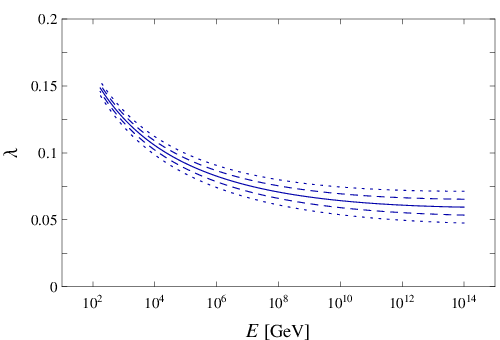
These curves show an important convergence property: the effects of the very large threshold corrections at are greatly reduced in the infrared. The quartic coupling is being strongly attracted towards an infrared quasi-fixed point so that, at the weak scale, the fractional uncertainty in the coupling is reduced by about a factor of . This convergence of the infrared flow reduces the sensitivity of the Higgs boson mass to
| (5) |
where has been arbitrarily normalized to . Note that the attraction is not quite so strong as to erase the sensitivity of low energy measurements to the value of the supersymmetric boundary condition. This therefore still allows us to probe the existence of supersymmetry at high scales.
In Figures 2 and 3 we have taken because, as we argued in the previous section, we expect supersymmetry breaking to be not far from the scale of unification, which from Figure 1 is seen to be of order . However, Figure 1 also shows that has large uncertainties, and the superparticle masses may not be exactly at . An uncertainty in the Higgs boson mass induced by varying from , however, is extremely small
| (6) |
as shown by the curves of Figure 4 for a fixed value of .

As increases above , it is apparent that the Higgs mass is remarkably insensitive to even large variations in . The Higgs mass changes by only when is changed by two orders of magnitude. The origin of this insensitivity can be seen from Figure 3; the curves for have a very small gradient above and, in addition, there is the convergence effect on scaling down to the weak scale.
We have seen that the predicted value of is rather insensitive to and , but what definition of should we choose, and what is the value of with that ? A convenient choice for is such that the leading-log contributions to from the superpartners and the heavy Higgs doublet vanishes. At the leading-log level, these threshold corrections are accounted for by choosing to match the full supersymmetric theory with the SM at an arbitrary scale , and inserting a term in proportional to for each superpartner that is integrated out. We can then make the choice of in such a way that the sum of these logarithmic terms vanishes.
In the appendix we compute the complete leading-log corrections to from all superpartners of SM particles and from the heavy Higgs doublet. We find that these corrections vanish if we choose to be
| (7) |
where and are the gaugino and top squark masses. An important point is that, although defined in this way does not exactly coincide with any particular superparticle mass, it is in the vicinity of and , so we expect to be not far from . Because the explicit dependence of on is very mild, this is enough to make a precise prediction for .
This choice of completely eliminates the leading-log supersymmetric corrections. The supersymmetric threshold correction, , therefore contains only finite terms. For example, the contribution from loops of top squarks at is
| (8) |
where is the trilinear coupling of the top squarks to the Higgs boson. The numerical size of this correction is much smaller than in the MSSM because, on scaling up to very large values of , the top Yukawa coupling is reduced by about a factor two and the effect is proportional to the fourth power of . For (), Eq. (8) gives (), leading to an increase of of () . We expect that the size of the other finite supersymmetric threshold corrections, which we have not computed, does not exceed this order. The effect of the supersymmetric correction is shown by the three solid red curves in Figure 4 for and .
Other threshold corrections may be present, depending on the nature of the theory near . The Higgs mass prediction will be affected by any additional significant couplings of the Higgs boson at or below . Except for the top coupling, which we have already included, the Yukawa couplings to the quarks and charged leptons give negligible effects. If neutrino masses are of Dirac type, then the neutrino Yukawa couplings are also very small and are irrelevant. However, for Majorana masses arising from the seesaw mechanism, there is the possibility of a correction to the Higgs mass if the right-handed neutrino mass, , is less than , in which case
| (9) |
where in the last expression we have taken , corresponding to the heaviest neutrino mass for the normal hierarchy spectrum. The correction is small; for and completely negligible for . In the special case , the correction rapidly grows, giving for , corresponding to a neutrino Yukawa coupling of . We stress that vanishes if right-handed neutrinos are above .
Having discussed the threshold corrections at the scale , we now turn to uncertainties that result from scaling between and . Indeed, at present the largest uncertainty in the Higgs mass prediction arises from the experimental uncertainties in and , which enter the RG equation for at one and two loops, respectively. The present uncertainty in leads to a uncertainty in the Higgs mass, as illustrated by the dashed curves of Figure 4. A conservative estimate of the uncertainty in is [12], leading to . A recent analysis of all relevant data argues that the uncertainty in is a factor three smaller [13].
The final uncertainties arise from higher loop effects in RG scaling and in the top quark threshold correction. First, the correction from three-loop QCD RG scaling decreases the Higgs mass by . We have not computed three-loop running from the top Yukawa coupling and , but do not expect these to be significantly larger than the three-loop QCD running. Second, in going from the top quark pole mass to the top Yukawa coupling, the QCD corrections reduce the Higgs mass by , and from one, two and three loops, respectively. As the loop level is increased, the successive reductions of the corrections by and suggest that the four-loop effect will be of order of the three-loop correction, i.e. . Hence, we arrive at a conservative estimate of the higher loop uncertainties in the Higgs mass prediction of .
Collecting these results leads to our final prediction for the Higgs boson mass in the SM
| (10) | |||||
where . As explained above, may vanish, so that only is mandatory; thus we have chosen to scale by a numerical factor following from Eq. (8). Our result shows that currently the largest uncertainties arise from the experimental error on and . The uncertainties from high energy theories are very small, and only about if we vary within two orders of magnitude from and take .
How might this situation change in the future? Studies at a future linear collider argue that the experimental uncertainties can be reduced to (defined at short distances) and [14], which induce uncertainties in the Higgs mass prediction of and , respectively. The same study estimates the experimental uncertainty in the Higgs boson mass to be , so that the confrontation of the prediction with experiment is now limited by from . With a Giga-Z sample, a linear collider may reach the much reduced uncertainty of [13]. Hence, in the future the prediction may take the form
| (11) | |||||
where experimental uncertainties are scaled by error bars. We have assumed sufficiently precise higher loop theoretical calculations, shifting the central value by , with .
So far we have assumed that is sufficiently less than that the boundary condition does not receive tree-level modifications from the enlargement of the SM gauge group, or threshold corrections, , from heavy states in the unified theory. If the unified gauge group is there is no tree-level correction, but is model dependent. Nevertheless, even when and are very close, it is reasonable for to be comparable to the threshold corrections required for gauge coupling unification, which are in , leading to . If then the prediction will depend on the form of the RG equations in the non-supersymmetric unified theory between and . Although these are model dependent, it is worth stressing that the effect of any such corrections on the Higgs mass will be reduced due to the IR focusing effect of the quasi-fixed point in the SM RG equation for .
If the SM gauge group is enlarged at by (), there is a tree-level modification to the boundary condition
| (12) |
where and are the gauge coupling and charge of the Higgs field. The last expression follows from taking equal to its unified value in , giving . This correction becomes power suppressed as the breaking scale is increased above .
3.2 Additional multiplets far below
The Higgs mass prediction of the previous section applied to the case that the effective theory below is the SM. How does the prediction change as additions are made to the low energy theory? For example, if experiment is able to confirm this prediction to within , can we conclude that there are likely no other states at the weak scale beyond the SM? We do not consider the possibility of adding light scalars below ; without an environmental selection, such scalars are extremely improbable in the landscape. Thus the scalar potential at the weak scale is that of the SM, with the physical Higgs boson mass depending on the single unknown parameter . How sensitive is this parameter to the addition of light fermions or gauge bosons?
The prediction does not survive if the SM gauge group is embedded in some larger group far below . For example, if the gauge group from to near the weak scale is , then the central value of the prediction changes. On the other hand, an additional gauge sector has no effect on the prediction if none of the new fermions carry SM quantum numbers, and if the SM particles are neutral under the new gauge interaction. The prediction will change if the Higgs boson or top quark carries the new gauge interaction and the new gauge coupling is not small.
Without extending the SM gauge group, the addition of light fermions will significantly modify the Higgs boson mass prediction if
- •
There are additional, large, renormalizable couplings involving either the Higgs boson or the top quark.
- •
The resulting additions to the beta function coefficients of the SM gauge interactions, , are significant.
While the former is model dependent, we can numerically study the latter in a rather model independent way.
If the additional fermions are all color singlets, contributions to increase the Higgs mass, as shown by the contours of Figure 5(a), where it is assumed that the mass of the additional fermions are .11 1 If the masses are reduced to , large additional corrections to the Higgs mass of order are induced, as the extra states give threshold corrections to the values of the gauge couplings extracted from data. These corrections rapidly decouple as the mass of the extra states increases, and are not included anywhere in this section.


The addition of a single vector-like lepton doublet increases the Higgs mass by about , and is marked with a dot. Note that is quantized in units of . In order for the Higgs boson mass to stay within of our prediction, only four additions with non-trivial are possible: one, two, or three vector-like doublets or one weak triplet. The case of one vector-like lepton doublet, shown by the dot in Figure 5(a), is particularly important, since it leads to gauge coupling unification that is as precise as for weak scale supersymmetry.
The most general theory with a single vector-like lepton doublet , with no singlets, is described by the Lagrangian
| (13) |
The new Yukawa coupling ensures that the heavy lepton is unstable, which is crucial since otherwise the theory is excluded by limits on the direct detection of DM. The charged and neutral heavy leptons, and , will be pair produced at colliders, and each decays to an electroweak boson and a lepton and .
An alternative possibility is that the vector-like lepton mixes with a neutral Majorana fermion so that, if the additional fermions are odd under some parity, the lightest neutral mass eigenstate is stable and, since it is Majorana, evades the DM direct detection limits. Indeed, these states result if the Higgsinos of the MSSM together with the bino or some other singlet fermion have masses far below [15]. In this case, new Yukawa interactions coupling the Higgs boson to the additional fermions may be present. In this theory, a Higgs mass prediction follows from a supersymmetric boundary condition on the quartic coupling [16], and depends on the size of the additional Yukawa interactions.
Adding colored fermions at the weak scale rapidly alters the Higgs mass prediction. For example, a single vector-like color triplet without electroweak quantum numbers reduces the Higgs mass prediction by about . In Figure 5(b) we show contours of the change in the Higgs mass prediction for the case of a single vector-like color triplet when there are also contributions to , coming from the colored triplet itself or from additional electroweak states. Two simple theories are shown by dots; one has states corresponding to multiplets , and the other has a further vector-like lepton doublet. This latter case has high precision gauge coupling unification and a Higgs mass prediction very close to the SM. If accessible, the colored triplet, , would be pair produced at the Tevatron or the LHC, with each decaying as via the Yukawa interaction . If mix with a singlet, the lightest state can be stable and contribute to DM. However, the colored state must still decay via , since if this interaction is absent can decay only via dimension six operators and is cosmologically stable.
Figure 5 shows that only a very few weak-scale multiplets with small SM charges can be added to the theory if the Higgs mass prediction is to survive at the level. Another possibility is to add multiplets at some scale intermediate between and . In the case that these states are non-colored, since the electroweak gauge couplings evolve slowly, Figure 5(a) is still approximately correct providing the axis labeling is changed from to . Twice as many multiplets can be placed at compared to . Adding colored states at had a large effect on the Higgs mass because, although the effect is two loop via the effect on the top Yukawa, the QCD coupling is large at the weak scale. By contrast, on adding states at intermediate scales, such as , the change in the Higgs mass is dominated by which gives an effect at one loop, rather than the two-loop effect from .
To conclude, experimental confirmation of the Higgs mass prediction of Eq. (10), to an accuracy of , removes almost all alternatives to the SM at the TeV scale. The addition of a vector-like lepton doublet remains as an interesting possibility.
3.3 Relation to other work
The theories illustrated by Figure 5 give a mild perturbation of less than about the SM Higgs mass prediction. The case of Split Supersymmetry [4] cannot be considered as a mild perturbation. Indeed Split Supersymmetry is taken to include a very wide ranges of and , so that the Higgs mass can range from the present experimental limit of up to about [17]. Taking very high does not yield a central value close to the SM prediction: the light gluino contribution to alone would decrease the Higgs mass prediction by about , but much more important are the new Yukawa couplings involving the Higgs boson, which increase the Higgs mass by to depending on and . For Split Supersymmetry with large and , a precise prediction for the Higgs mass emerges
| (14) |
The precision of this special value of the Higgs mass within Split Supersymmetry can be defended at a level similar to that of Eq. (10) for the SM. Indeed, the threshold corrections involving electroweak gauginos are now at the weak scale, and could potentially be determined by measuring the electroweak gaugino masses and couplings.
Motivated by Split Supersymmetry, several groups have investigated supersymmetry breaking at a high scale, including models with supersymmetry breaking at a Peccei-Quinn breaking scale of [18] and models with gauge coupling unification at via non- hypercharge normalization [19]. In these models, a supersymmetric boundary condition on the quartic coupling yields a Higgs mass prediction and, for large values of and taking account different values of the top quark mass, these predictions are not far from our central value of . This is a reflection of the remarkable insensitivity of the Higgs mass to variations in the unified scale and threshold corrections, as given in Eqs. (5) and (6). Indeed, it will be difficult to use the Higgs mass prediction to distinguish between these schemes—for example, changing the unification scale from to changes the Higgs mass by less than . Furthermore, the supersymmetric boundary condition on the Higgs quartic coupling does not depend on the Kac-Moody level relevant for gauge coupling unification. On the other hand, the Higgs mass decreases significantly at low values of , as shown in Figure 2, so that there is sensitivity to models that predict particular low values of [20].
4 Theories with High Scale Supersymmetry Breaking
We have explored the consequences of taking the SM as the correct effective theory up to some very high scale of supersymmetry breaking , where the unification scale , as illustrated in Figure 1. What is the new physics that emerges at this scale? Since supersymmetry and the multiverse are both motivated by string theory, it is plausible that the higher dimensions of space are being encountered. This offers the elegant possibility that breaking of both unified gauge symmetry and supersymmetry are associated with these extra dimensions; in particular, the unified gauge symmetry may be broken intrinsically by the compactification. While a solution to the doublet-triplet splitting problem is no longer needed, such a framework has many appealing phenomenological features:
- •
Proton stability is naturally accounted for, without the need for imposing any additional symmetries. Since supersymmetry is broken at the high scale, there is no need to impose parity to avoid proton decay at dimension 4. Indeed, proton stability is automatic at both dimension 4 and 5. With four-dimensional (4D) unification at , proton decay from gauge-mediated dimension 6 operators are disastrous, but this is easily avoided in higher dimensional theories [21].
- •
In simple theories the boundary conditions in extra dimensions, which involve very few parameters, can break both unified gauge symmetry and supersymmetry. This gives simple KK towers of superpartners and unified states, allowing the calculation of threshold corrections to both gauge coupling unification and the Higgs quartic coupling.
- •
The requirement of two independent Higgs fields is removed: although different states of the supersymmetric theory couple to up and down quark sectors, these states may be part of the same supermultiplet in higher dimensions [22].
- •
The Higgs boson can be a slepton, allowing a unification of the matter and Higgs sectors of the SM. This is not possible with low energy supersymmetry because of the masses and interactions that accompany the associated parity violation, but these constraints decouple as the scale of supersymmetry is raised.
In section 4.1 we show that, in theories where the boundary condition takes the form of Eq. (2), an approximate symmetry, whether originating in four or more dimensions, leads to a sufficiently large that the precise Higgs mass prediction of Fig. 4 applies, with a very small correction from of Eq. (4). In section 4.2 we present a new, distinct class of theories which is particularly interesting in the context of high scale supersymmetry breaking. In these theories, does not exist and the boundary condition is given by Eq. (3). Although the Higgs boson mass in these theories can receive somewhat larger uncertainties than the ones discussed in section 3.1, they are still at the level of a GeV.
4.1 An approximate Peccei-Quinn symmetry
In the case that the supersymmetric theory at is 4D, or that the two Higgs doublets of the supersymmetric theory, , arise from different supermultiplets of a higher dimensional theory, the SM Higgs doublet is a linear combination of
| (15) |
The boundary condition on the SM Higgs quartic coupling is then given by Eq. (2) and depends on the mixing angle . However, for the Higgs boson mass becomes very insensitive to , varying by less than . A mechanism for large can therefore lead to a very tight prediction for the Higgs boson mass.
If the theory possesses an approximate Peccei-Quinn symmetry, then the Higgsino mass parameter is suppressed, , and the mass matrix for the Higgs doublets takes the generic form
| (16) |
where is the small symmetry breaking parameter. The parameters are typically of order and scan independently in the multiverse. Given that environmental selection requires one eigenvalue of the above matrix to be of order , what is the most probable value of we observe? In particular, is it more probable to have the determinant nearly vanish by having both suppressed by , giving , or by having one of them suppressed by , so that ? (We ignore the possibility of since this is experimentally disfavored.) It turns out that the case of is less probable by a factor of , since it implies that the heavier mass-squared eigenvalue is of order , requiring extra fine-tuning beyond that necessary to obtain the weak scale. Hence, the approximate symmetry leads to the expectation
| (17) |
How small might be? With dimensionless couplings of order unity, the bottom to top quark mass ratio takes the form
| (18) |
where the first term arises from the quark Yukawa coupling while the second term represents a possible contribution from higher dimension operators , where or to preserve the boundary condition on , as discussed in section 2. Thus the approximate Peccei-Quinn symmetry leads to an understanding of the small ratio for any
| (19) |
Conservatively, taking the upper limit to be leads to a contribution from to the Higgs boson mass of only and, for most values of that lead to an understanding for , the contribution from is negligible. Indeed, it is interesting to note that may be extremely small so that, for all practical purposes, and the quark mass originates entirely from the higher dimension operator. In this case the Higgsino becomes light, and may be the vector-like lepton doublet of Eq. (13).
The Peccei-Quinn symmetry described here may be responsible for the solution to the strong problem, in which case we expect , where is the axion decay constant, the scale at which the Peccei-Quinn symmetry is spontaneously broken. For example, this could result from a 4D superpotential interaction of the type , with order unity coupling and the scalar component of acquiring a VEV of size . This would lead to as well as the suppressed Peccei-Quinn breaking mass in Eq. (16). With and , one expects , so that the correction to the Higgs mass prediction from is negligible.
In theories with extra spatial dimensions, the Higgs fields have profiles in the bulk, and the small parameter may result from a small overlap of the wavefunctions for and . In this case, there is no need to impose an approximate symmetry on the higher dimensional theory; rather, it emerges in the 4D theory as a result of locality in the higher dimensions. This origin for the small off-diagonal term in Eq. (16) is somewhat general; no matter how many extra dimensions, a small results providing and profiles are peaked in differing locations. Strong peaking of the wavefunctions might arise, for example, from higher dimensional mass terms or from localizations on background fields with kink solutions. In fact, this suppression of the mass term is unique among the supersymmetry breaking masses of the MSSM states: once the gauginos have a large mass, the squark, slepton and diagonal Higgs mass terms cannot be protected from low-energy radiative corrections, while the Higgsino and off-diagonal Higgs mass terms can be.
A simple example accommodating the above mechanism occurs in a supersymmetric theory in 5D, with the unified symmetry broken by boundary conditions on the orbifold [23, 21]. Supersymmetry may be broken on one of the branes by the highest component VEV of a chiral superfield . By localizing towards the brane where resides, while towards the other, we can obtain the pattern of the Higgs mass matrix in Eq. (16). The quark and lepton fields propagate in the bulk, so that the up-type and down-type Yukawa couplings arise from the branes where and are localized, respectively. Dangerous dimension six proton decay due to gauge boson exchange is also avoided if the matter fields are in the bulk because of the split-multiplet structure. An alternative possibility to break supersymmetry is by the -component VEV of the radius modulus, or equivalently, through nontrivial boundary conditions [24, 25]. The pattern of Eq. (16) can also be obtained in this case, by having a similar configuration for the Higgs and matter fields in the extra dimension.
4.2 Models with a single Higgs supermultiplet
In general, the SM Higgs boson is a linear combination of states at the scale . There is, however, an interesting possibility that it comes from a single supermultiplet in higher dimensions. Consider, for example, a supersymmetric gauge theory in 5D, with the extra dimension compactified on : . We introduce three generations of quark and lepton hypermultiplets ( and ) and a single Higgs hypermultiplet in the bulk, with the boundary conditions
| (20) |
Here, we have denoted a hypermultiplet in terms of two 4D chiral superfields, and the first and second signs in parentheses represent boundary conditions at and , respectively ( for Neumann and for Dirichlet). To cancel brane-localized gauge anomalies induced by , we also introduce an “inert Higgs” hypermultiplet , which has the same boundary conditions but the opposite quantum numbers as . This multiplet, however, does not lead to any low energy consequences.
Without supersymmetry breaking, the spectrum of the low energy theory consists of 4D vector supermultiplets () and three generations of quark and lepton chiral supermultiplets . The KK towers of these states have masses (), while those of the and hypermultiplets have (). We now introduce supersymmetry breaking via the -component VEV of the radius modulus, or through nontrivial boundary conditions. This shifts the tree-level spectrum of low-lying states as
| (21) |
where () is the parameter specifying the strength of supersymmetry breaking [25], and the component fields are defined by , (and similarly for ), , and . For , this is essentially the theory of Ref. [22]. An important difference, however, is that we now take the compactification scale to be around the unified scale, rather than at the TeV scale, so that the (and ) states generically obtain masses of order at one loop, which are much larger than the weak scale. However, environmental selection can still set to be of order the weak scale by adjusting various contributions to (for example by making deviate slightly from or by introducing 5D masses for bulk fields; see below). The low energy particle content is then exactly that of the SM:
| (22) |
All the other states decouple at the scale .
The Yukawa couplings are obtained by introducing brane-localized operators
| (23) |
where is the cutoff scale of the theory, which we take to be a factor of a few larger than . The SM Higgs boson, , lies in the scalar components of and as
| (24) |
so that the 4D Yukawa couplings are given by
| (25) |
with . Here, we have assumed vanishing 5D masses for the bulk hypermultiplets. The form of Eq. (25) is precisely that of the SM.
How does the selection of work? In the limit of and vanishing 5D masses, the dominant radiative correction to comes from top quark/squark loops
| (26) |
where we have used , evaluated at . Therefore, by making slightly deviate from
| (27) |
we can set to have the correct, weak scale (and negative) value.22 2 The precise value of would be changed by the existence of brane-localized terms, such as , but our basic conclusion does not change. Below we assume that these terms are absent. Alternatively, we may introduce 5D bulk masses for top hypermultiplets. In this case the top-loop contribution of Eq. (26) is suppressed [26], so that it can be canceled with the gauge loop contribution
| (28) |
even for , leaving the correct value for .
An interesting property of the theory considered here is that the tree-level Higgs quartic coupling is given by
| (29) |
regardless of the value of —there is no free parameter such as in 4D supersymmetric theories. This is a consequence of the symmetry and the fact that the SM Higgs boson resides in a single higher dimensional supermultiplet. Therefore, at the leading order, the theory just below is precisely the SM but with the Higgs quartic coupling constrained as in Eq. (29). The relation of Eq. (29) can receive corrections from brane-localized kinetic terms. These effects are suppressed by the volume factor (and possibly also by a loop factor), which we estimate to give an correction to . This is translated into an uncertainty of the Higgs mass prediction at the level of a GeV.
It is straightforward to construct unified models along the lines discussed here. For example, we can consider a supersymmetric theory in 6D with broken along one extra dimension while supersymmetry along the other. For , we can even use the same dimension to break both supersymmetry and a unified symmetry. We simply need to embed the model discussed above into , and break by boundary conditions at (and supersymmetry by Eq. (27)). In this theory, some of the unified states have a tree-level mass of and thus lighter than by about an order of magnitude, and the colored triplet Higgsinos obtain their masses through brane-localized operators. Unification of the SM gauge couplings receives corrections both from KK towers and brane-localized gauge kinetic operators. The deviation from single-scale exact unification in the SM may arise from these corrections.
5 Evidence for the Multiverse from the Higgs Boson Mass
The Standard Model is remarkably successful, correctly predicting the results of three decades of particle physics experiments at both the high energy and high precision frontiers. From the absence of proton decay, to precision measurements of the electroweak sector, to rare quark and lepton flavor violation and even violation, the SM has consistently and repeatedly passed every experimental challenge. Indeed, the electroweak and flavor data now constrain new physics at the TeV scale so strongly, that the resulting difficulties in developing alternative natural theories have become a main focus of much research. Why then do we resist the simplest possibility, that the SM is the correct description of nature up to unified energy scales? This question seems particularly pressing since the SM, valid to very high energies, predicts , precisely the range selected by limits from direct searches and from precision electroweak data.
There are two key deficiencies of the SM, one theoretical and one observational. On the theoretical side, the lack of naturalness of the Higgs mass parameter has been the essential driving force for a variety of extensions of the theory at the TeV scale. However, the cosmological constant is a numerically more severe fine-tuning problem, and has no known symmetry solution. The realization that this problem has an environmental solution [5] motivated the discovery of a possible environmental understanding for the weak scale [2]. The discovery of dark energy [27] provided remarkable evidence for environmental selection: dark energy with is a necessary consequence of the environmental solution of the cosmological constant problem, and requires no physics beneath unified scales beyond the SM and general relativity. The absence of dark energy would have demonstrated that environmental selection had failed its greatest opportunity. Of course, an enormous landscape of vacua is required, as well as a cosmological mechanism for populating these vacua to form a multiverse. The realization that string theory [7] and eternal inflation [28] may yield such a multiverse, opens the door to a firm theoretical foundation for the environmental selection of both the cosmological constant and the weak scale.
Dark matter provides the other key deficiency of the SM, but it is a theoretical extrapolation to attribute this DM to particles with weak scale mass. Even if DM is composed of cold particles, nothing is known observationally about their mass. The WIMP hypothesis provides an intriguing possibility that the abundance of DM may be derived from the weak scale, but is subject to uncertainties of several orders of magnitude. If the SM is valid to unified scales, the most compelling candidate for DM is axions. The strong problem requires a symmetry solution, since there is no environmental need for low . The axion solution, theoretically motivated by string theory, cannot be implemented at the weak scale, and requires . Even if is as large as the unified scale, environmental selection can act on the initial axion misalignment angle to avoid overproduction of DM [10].
Over more than three decades, much effort has been expended on extensions of the SM at the TeV scale. Is there any experimental evidence that any of these alternatives are to be preferred over the SM? While there is no direct experimental evidence for any such extension, in the case of weak scale supersymmetry gauge coupling unification occurs with greater precision than in the SM. When first discovered at LEP, this result appeared highly significant. Precise data outweighed the well-known cosmological and flavor problems of supersymmetry, which received renewed attention. However, the LEP2 limit on the Higgs boson mass provided contrary data, that imposed a precise numerical naturalness problem on supersymmetry. Is the reduction of the unified threshold corrections on gauge coupling unification by an order of magnitude worth the required fine-tuning of the theory at the percent level?
With environmental selection on a multiverse, the minimal effective theory below the unified scale, SM GR, has no deficiencies. Instead of introducing problems by augmenting the SM at the TeV scale, it seems worthwhile seeking additional evidence for environmental selection in the minimal effective theory. In this paper we presented a precise and robust prediction for the Higgs boson mass. We argued that a supersymmetric boundary condition on the Higgs quartic coupling is likely, yielding a Higgs boson mass range of . The upper edge of is particularly interesting, arising from the special situation that the SM Higgs boson lies dominantly in a single supermultiplet as occurs, for example, with an approximate Peccei-Quinn symmetry. Corrections at the supersymmetry breaking scale are remarkably small: from top squark loops and from varying by two orders of magnitude. The dominant uncertainty in the prediction, of , arises from the present uncertainties in and , but measurements at future collider experiments could reduce this to , so that the prediction could be tested down to the level of .
Going beyond this minimal scenario, there are several physical origins of corrections in the GeV region. If neutrino masses arise from the seesaw mechanism, the corrections to the Higgs boson mass are negligible except, in a certain region of parameter space with , the Higgs mass could be raised by about a GeV.33 3 This implies that leptogenesis [29] can be accommodated without affecting the Higgs mass prediction. Higher dimensional theories having a single Higgs supermultiplet lead to the Higgs mass being near the upper edge of , but brane-localized kinetic terms lead to uncertainties of about a GeV. Finally, while adding states at the weak scale beyond those of the SM typically destroys the prediction, there are a few minimal cases that yield mild perturbations; for example, a single vector-like lepton increases the Higgs boson mass only by .
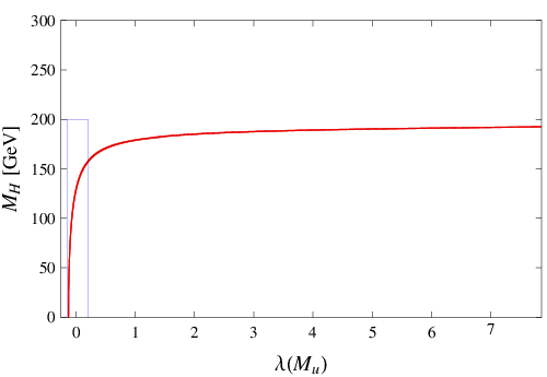
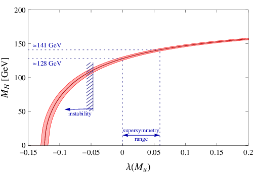
Are there other special values for the Higgs boson mass that would provide evidence for the multiverse? In Figure 6 we show the Higgs mass as a function of the quartic coupling at the unified scale , assuming only that the effective theory below is the SM. The left panel gives a wide range of , while the right panel expands the region of small . We draw attention to four special values of the Higgs mass:44 4 To simplify the presentation, we take the scale at which the quartic coupling takes special values to be . In fact, depending on the case, this scale could be or , but we do not expect these scales to differ by many orders of magnitude.
- •
: results from a very wide range of , including the case of strong coupling, .
- •
: results from the supersymmetric boundary condition , as explored in detail in this paper.
- •
: results from .
- •
: this is the smallest Higgs boson mass theoretically allowed, since smaller values would lead to cosmological instabilities in the electroweak vacuum. A value close to this may result from a multiverse distribution function that is peaked strongly towards large and negative [30].
Since is not well determined by gauge coupling unification, an important question is the sensitivity of these four special Higgs mass values to variations in . In the first three cases the sensitivity depends on how close the RG trajectory is to the quasi-fixed point trajectory. The case of strong coupling is very far from the fixed point and has significant sensitivity, with the Higgs mass varying by for . A Higgs mass in this range would be indicative of a multiverse that has a high probability for a large quartic coupling, but the evidence would be rather weak. The cases of and are much closer to the quasi-fixed point, giving Higgs mass variations of only and , respectively, for the same variation in . Thus a Higgs mass near would provide strong evidence for the multiverse, although not quite as strong as might occur for a value near . The case of the smallest Higgs mass is more complicated, since it involves tunneling, but it is also insensitive to variations in . Thus a value of the Higgs mass very close to the minimal value would also yield evidence for the multiverse, although for this to occur requires a very sharp variation in the multiverse probability distribution for .
Although this paper has focused on the Higgs boson mass near , a value near is also very interesting. These two values are the upper and lower edge values allowed by the supersymmetric boundary condition of Eq. (2), corresponding to and respectively. Studying the mass matrix for the two Higgs doublets in the supersymmetric theory, the former occurs when a diagonal entry is much larger than the off-diagonal entry, while the latter occurs if the off-diagonal entry is much larger than the splitting between the diagonal entries, as would occur if the mass matrix were invariant under a symmetry that interchanged the two doublets. Our discussions of the corrections to the Higgs mass for the large case apply also to the case of near unity except, as noted above, the convergence effect from the quasi-fixed point of the quartic coupling is not quite as strong. For example, the top squark loops at lead to an uncertainty in the Higgs mass of for . Also the uncertainty in the Higgs mass arising from the present experimental uncertainties on and is , larger than at the edge. Finally we should note that a Higgs mass near occurs in any theory where the SM Higgs doublet is a pseudo Nambu-Goldstone boson, with a vanishing tree-level potential at . An example of this occurs when the Higgs boson is identified as an extra-dimensional component of a gauge field in a non-supersymmetric 5D theory [31].
Much of the excitement in particle physics in the coming decade will follow from unraveling the origin of the weak scale. Three clear options are
- •
Weak scale supersymmetry. This will confirm the indirect evidence of gauge coupling unification, and allow many measurements that provide a window to much higher energy scales.
- •
New strong dynamics. A composite Higgs, or even a Higgsless theory, would make the TeV scale extremely rich, and may even herald new spatial dimensions.
- •
Environmental selection. Precision measurements of SM parameters may point to a multiverse and the need for a clearer understanding of the catastrophic boundaries at which selection takes place.
Strong evidence for the multiverse would result if the LHC discovered a Higgs boson mass close to , or , and no new physics beyond the SM. This would add greatly to the evidence from the cosmological constant problem and the discovery of dark energy. The two fine-tuning problems of SM GR would have a common solution, with other solutions either unknown or disproved. Through nuclear stability, the multiverse accounts for the values of the up quark, down quark and electron masses remarkably well [32]. Furthermore, the multiverse may also explain the cosmological mystery of why the time scales of structure formation, galaxy cooling and vacuum domination do not differ by many orders of magnitude, but are all comparable to the present age of the universe [33]. Instead of discovering more symmetries, the LHC may play a key part in the accumulation of evidence for more universes.
Acknowledgments
We thank Gilly Elor and Piyush Kumar for useful discussions. This work was supported in part by the Director, Office of Science, Office of High Energy and Nuclear Physics, of the US Department of Energy under Contract DE-AC02-05CH11231. The work of L.H. was supported in part by the National Science Foundation under grant PHY-0457315, and that of Y.N. under grants PHY-0555661 and PHY-0855653.
Appendix A Supersymmetric Threshold Corrections at
The leading-log corrections to the supersymmetric boundary condition, , when matching between the SM and a theory with the states of the MSSM, at a scale , are
| (30) | |||||
where , , (), and are the gaugino, Higgsino, squark and slepton, and heavy Higgs boson masses, , and (). Here, we have taken the wino and bino masses to be equal, , which is generically a good approximation since is not far from . The dependence on the matching scale cancels that from the RG scaling in the SM, given by (6).
Since , it is appropriate to make an approximation , leading to
| (31) | |||||
As discussed in section 3.1, a useful choice of is the one that makes vanish. This scale can be estimated by assuming that the second line of Eq. (31) is dominated by the gaugino piece:
| (32) |
where , and we have taken . The logarithmic terms for each particle dropped from the second line of Eq. (31) have coefficients that are smaller than in the gaugino term by a factor of or more. In fact, a random deviation of these superparticle masses from by a similar amount to and will not contribute to as much as the terms shown in Eq. (32). By equating the expression of Eq. (32) to zero, we obtain
| (33) |
This is the expression quoted in Eq. (7).
References
- [1] H. Georgi, H. R. Quinn and S. Weinberg, Phys. Rev. Lett. 33, 451 (1974).
- [2] V. Agrawal, S. M. Barr, J. F. Donoghue and D. Seckel, Phys. Rev. D 57, 5480 (1998) [arXiv:hep-ph/9707380].
- [3] T. Damour and J. F. Donoghue, Phys. Rev. D 78, 014014 (2008) [arXiv:0712.2968 [hep-ph]].
- [4] N. Arkani-Hamed and S. Dimopoulos, JHEP 06, 073 (2005) [arXiv:hep-th/0405159].
- [5] S. Weinberg, Phys. Rev. Lett. 59, 2607 (1987).
- [6] E. Komatsu et al. [WMAP Collaboration], Astrophys. J. Suppl. 180, 330 (2009) [arXiv:0803.0547 [astro-ph]]; M. Kowalski et al. [Supernova Cosmology Project Collaboration], Astrophys. J. 686, 749 (2008) [arXiv:0804.4142 [astro-ph]].
- [7] R. Bousso and J. Polchinski, JHEP 06, 006 (2000) [arXiv:hep-th/0004134]; S. Kachru, R. Kallosh, A. Linde and S. P. Trivedi, Phys. Rev. D 68, 046005 (2003) [arXiv:hep-th/0301240]; L. Susskind, arXiv:hep-th/0302219; M. R. Douglas, JHEP 05, 046 (2003) [arXiv:hep-th/0303194].
- [8] R. D. Peccei and H. R. Quinn, Phys. Rev. Lett. 38, 1440 (1977).
- [9] S. Weinberg, Phys. Rev. Lett. 40, 223 (1978); F. Wilczek, Phys. Rev. Lett. 40, 279 (1978).
- [10] A. D. Linde, Phys. Lett. B 201, 437 (1988); F. Wilczek, arXiv:hep-ph/0408167; M. Tegmark, A. Aguirre, M. J. Rees and F. Wilczek, Phys. Rev. D 73, 023505 (2006) [arXiv:astro-ph/0511774].
- [11] The Tevatron Electroweak Working Group, arXiv:0903.2503 [hep-ex].
- [12] C. Amsler et al. [Particle Data Group], Phys. Lett. B 667, 1 (2008).
- [13] S. Bethke, arXiv:0908.1135 [hep-ph].
- [14] T. Abe et al. [American Linear Collider Working Group], arXiv:hep-ex/0106055; arXiv:hep-ex/0106056; arXiv:hep-ex/0106057; arXiv:hep-ex/0106058, and references therein.
- [15] N. Arkani-Hamed, S. Dimopoulos and S. Kachru, arXiv:hep-th/0501082; R. Mahbubani and L. Senatore, Phys. Rev. D 73, 043510 (2006) [arXiv:hep-ph/0510064].
- [16] G. Elor, H.-S. Goh, L. J. Hall, P. Kumar and Y. Nomura, to appear.
- [17] M. Binger, Phys. Rev. D 73, 095001 (2006) [arXiv:hep-ph/0408240].
- [18] V. Barger, C.-W. Chiang, J. Jiang and T. Li, Nucl. Phys. B 705, 71 (2005) [arXiv:hep-ph/0410252].
- [19] V. Barger, J. Jiang, P. Langacker and T. Li, Phys. Lett. B 624, 233 (2005) [arXiv:hep-ph/0503226]; Nucl. Phys. B 726, 149 (2005) [arXiv:hep-ph/0504093]; D. Emmanuel-Costa and R. González Felipe, Phys. Lett. B 623, 111 (2005) [arXiv:hep-ph/0505257].
- [20] I. Gogoladze, T. Li and Q. Shafi, Phys. Rev. D 73, 066008 (2006) [arXiv:hep-ph/0602040].
- [21] L. Hall and Y. Nomura, Phys. Rev. D 64, 055003 (2001) [arXiv:hep-ph/0103125].
- [22] R. Barbieri, L. J. Hall and Y. Nomura, Phys. Rev. D 63, 105007 (2001) [arXiv:hep-ph/0011311].
- [23] Y. Kawamura, Prog. Theor. Phys. 105, 999 (2001) [arXiv:hep-ph/0012125].
- [24] J. Scherk and J. H. Schwarz, Phys. Lett. B 82, 60 (1979); Nucl. Phys. B 153, 61 (1979); D. E. Kaplan and N. Weiner, arXiv:hep-ph/0108001.
- [25] R. Barbieri, L. J. Hall and Y. Nomura, Nucl. Phys. B 624, 63 (2002) [arXiv:hep-th/0107004].
- [26] R. Barbieri, L. J. Hall, G. Marandella, Y. Nomura, T. Okui, S. J. Oliver and M. Papucci, Nucl. Phys. B 663, 141 (2003) [arXiv:hep-ph/0208153].
- [27] S. Perlmutter et al. [Supernova Cosmology Project Collaboration], Astrophys. J. 517, 565 (1999) [arXiv:astro-ph/9812133]; A. G. Riess et al. [Supernova Search Team Collaboration], Astron. J. 116, 1009 (1998) [arXiv:astro-ph/9805201].
- [28] A. H. Guth and E. J. Weinberg, Nucl. Phys. B 212, 321 (1983); A. Vilenkin, Phys. Rev. D 27, 2848 (1983); A. D. Linde, Phys. Lett. B 175, 395 (1986); Mod. Phys. Lett. A 1, 81 (1986).
- [29] M. Fukugita and T. Yanagida, Phys. Lett. B 174, 45 (1986).
- [30] B. Feldstein, L. J. Hall and T. Watari, Phys. Rev. D 74, 095011 (2006) [arXiv:hep-ph/0608121].
- [31] I. Gogoladze, N. Okada and Q. Shafi, Phys. Lett. B 655, 257 (2007) [arXiv:0705.3035 [hep-ph]].
- [32] L. J. Hall and Y. Nomura, Phys. Rev. D 78, 035001 (2008) [arXiv:0712.2454 [hep-ph]]; C. J. Hogan, Rev. Mod. Phys. 72, 1149 (2000) [arXiv:astro-ph/9909295], and references therein.
- [33] R. Bousso, L. J. Hall and Y. Nomura, Phys. Rev. D 80, 063510 (2009) [arXiv:0902.2263 [hep-th]].