跳到论文正文
W Papers独立论文阅读器 arXiv:0910.2045 论文正文 计算阅读时间 · 0%
引用这篇论文根据当前论文元数据生成,正式投稿前建议核对。


License: arXiv.org perpetual non-exclusive license
arXiv:0910.2045v2 [math-ph] 16 May 2011

Universality in the 2D Ising model
and conformal invariance of fermionic observablesThanks: A St.Petersburg Department of Steklov Mathematical Institute (PDMI RAS). Fontanka 27, 191023 St.Petersburg, Russia.Thanks: B Section de Mathématiques, Université de Genève. 2-4 rue du Lièvre, Case postale 64, 1211 Genève 4, Suisse.Thanks: C Chebyshev Laboratory, Department of Mathematics and Mechanics, Saint-Petersburg State University, 14th Line, 29b, 199178 Saint-Petersburg, Russia.Thanks: E-mail addresses: dchelkak@pdmi.ras.ru, Stanislav.Smirnov@unige.ch

Dmitry Chelkaka,c and Stanislav Smirnovb,c
Date: August 24, 2026
Abstract.

It is widely believed that the celebrated 2D Ising model at criticality has a universal and conformally invariant scaling limit, which is used in deriving many of its properties. However, no mathematical proof has ever been given, and even physics arguments support (a priori weaker) Möbius invariance. We introduce discrete holomorphic fermions for the 2D Ising model at criticality on a large family of planar graphs. We show that on bounded domains with appropriate boundary conditions, those have universal and conformally invariant scaling limits, thus proving the universality and conformal invariance conjectures.

Key words and phrases: 
Ising model, universality, conformal invariance, discrete analytic function, fermion, isoradial graph
1991 Mathematics Subject Classification
82B20, 60K35, 30C35, 81T40

1. Introduction

1.1. Universality and conformal invariance in the Ising model

1.1.1. Historical background

The celebrated Lenz-Ising model is one of the simplest systems exhibiting an order–disorder transition. It was introduced by Lenz in [Len20], and his student Ising proved [Isi25] in his PhD thesis the absence of phase transition in dimension one, wrongly conjecturing the same picture in higher dimensions. This belief was widely shared, and motivated Heisenberg to introduce his model [Hei28]. However, some years later Peierls [Pei36] used estimates on the length of interfaces between spin clusters to disprove the conjecture, showing a phase transition in the two dimensional case. After Kramers and Wannier [KW41] derived the value of the critical temperature and Onsager [Ons44] analyzed behavior of the partition function for the Ising model on the two-dimensional square lattice, it became an archetypical example of the phase transition in lattice models and in statistical mechanics in general, see [Nis05, Nis09] for the history of its rise to prominence.

Over the last six decades, thousands of papers were written about the Ising model, with most of the literature, including this paper, restricted to the two dimensional case (similar behavior is expected in three dimensions, but for now the complete description remains out of reach). The partition function and other parameters were computed exactly in several different ways, usually on the square lattice or other regular graphs. It is thus customary to say that the 2D Ising model is exactly solvable, though one should remark that most of the derivations are non-rigorous, and moreover many quantities cannot be derived by traditional methods.

Arrival of the renormalization group formalism (see [Fis98] for a historical exposition) led to an even better physical understanding, albeit still non-rigorous. It suggests that block-spin renormalization transformation (coarse-graining, i.e., replacing a block of neighboring sites by one) corresponds to appropriately changing the scale and the temperature. The Kramers-Wannier critical point arises then as a fixed point of the renormalization transformations, with the usual picture of stable and unstable directions.

In particular, under simple rescaling the Ising model at the critical temperature should converge to a scaling limit – a “continuous” version of the originally discrete Ising model, which corresponds to a quantum field theory. This leads to the idea of universality: the Ising models on different regular lattices or even more general planar graphs belong to the same renormalization space, with a unique critical point, and so at criticality the scaling limit and the scaling dimensions of the Ising model should be independent of the lattice (while the critical temperature depends on it). Being unique, the scaling limit at the critical point is translation and scale invariant, which allows to deduce some information about correlations [PP66, Kad66]. By additionally postulating invariance under inversions, one obtains Möbius invariance, i.e. invariance under global conformal transformations of the plane, which allows [Pol70] to deduce more. In seminal papers [BPZ84a, BPZ84b] Belavin, Polyakov and Zamolodchikov suggested much stronger full conformal invariance (under all conformal transformations of subregions), thus generating an explosion of activity in conformal field theory, which allowed to explain non-rigorously many phenomena, see [ISZ88] for a collection of the founding papers of the subject. Note that in the physics literature there is sometimes confusion between the two notions, with Möbius invariance often called conformal invariance, though the latter is a much stronger property.

Over the last 25 years our physical understanding of the 2D critical lattice models has greatly improved, and the universality and conformal invariance are widely accepted by the physics community. However, supporting arguments are largely non-rigorous and some even lack physical motivation. This is especially awkward in the case of the Ising model, which indeed admits many exact calculations.

1.1.2. Our results

The goal of this paper is to construct lattice holomorphic fermions and to show that they have a universal conformally invariant scaling limit. We give unambiguous (and mathematically rigorous) arguments for the existence of the scaling limit, its universality and conformal invariance for some observables for the 2D Ising model at criticality, and provide the framework to establish the same for all observables. By conformal invariance we mean not the Möbius invariance, but rather the full conformal invariance, or invariance under conformal transformations of subregions of ℂ{\mathbb{C}}. This is a much stronger property, since conformal transformations form an infinite dimensional pseudogroup, unlike the Möbius ones. Working in subregions necessarily leads us to consider the Ising model in domains with appropriate boundary conditions.

At present we cannot make rigorous the renormalization approach, but we hope that the knowledge gained will help to do this in the future. Rather, we use the integrable structure to construct discrete holomorphic fermions in the Ising model. For simplicity we work with discrete holomorphic functions, defined e.g. on the graph edges, which when multiplied by the d​z\sqrt{dz} field become fermions or spinors. Those functions turn out to be discrete holomorphic solutions of a discrete version of the Riemann-Hilbert boundary value problem, and we develop appropriate tools to show that they converge to their continuous counterparts, much as Courant, Friedrichs and Lewy have done in [CFL28] for the Dirichlet problem. The continuous versions of our boundary value problems are d​z\sqrt{dz}-covariant, and conformal invariance and universality then follow, since different discrete conformal structures converge to the same universal limit.

Starting from these observables, one can construct new ones, describe interfaces by the Schramm’s SLE curves, and prove and improve many predictions originating in physics. Moreover, our techniques work off criticality, and lead to massive field theories and SLEs. Several possible developments will be the subject of our future work [CS11, Smi11, KS11, HS09].

We will work with the family of isoradial graphs or equivalently rhombic lattices. The latter were introduced by Duffin [Duf68] in late sixties as (perhaps) the largest family of graphs for which the Cauchy-Riemann operator admits a nice discretization. They reappeared recently in the work of Mercat [Mer01] and Kenyon [Ken02], as isoradial graphs – possibly the largest family of graphs were the Ising and dimer models enjoy the same integrability properties as on the square lattice: in particular, the critical point is well defined, with weights depending only on the local structure. More recently, Boutilier and de Tilière [BdT08, BdT09] used the Fisher representation of the Ising model by dimers and Kenyon’s techniques to calculate, among other things, free energy for the Ising model on isoradial graphs. While their work is closely related to ours (we can too use the Fisher representation instead of the vertex operators to construct holomorphic fermions), they work in the full plane and so do not address conformal invariance. Note that earlier eight vertex and Ising models were considered by Baxter [Bax78] on ZZ-invariant graphs, arising from planar line arrangements. Those graphs are topologically the same as the isoradial graphs, and the choice of weights coincides with ours, so quantities like partition function would coincide. Kenyon and Schlenker [KS05] have shown that such graphs admit isoradial embeddings, but those change the conformal structure, and one does not expect conformal invariance for the Ising model on general ZZ-invariant graphs.

So there are two reasons for our choice of this particular family: firstly it seems to be the largest family where the Ising model we are about to study is nicely defined, and secondly (and perhaps not coincidentally) it seems to be the largest family of graphs where our main tools, the discrete complex analysis, works well. It is thus natural to consider this family of graphs in the context of conformal invariance and universality of the 2D Ising model scaling limits.

The fermion we construct for the random cluster representation of the Ising model on domains with two marked boundary points is roughly speaking given by the probability that the interface joining those points passes through a given edge, corrected by a complex weight. The fermion was proposed in [Smi06, Smi07] for the square lattice (see also independent [RC06] for its physical connections, albeit without discussion of the boundary problem and covariance). The fermion for the spin representation is somewhat more difficult to construct, it corresponds to the partition function of the Ising model with a z\sqrt{z} monodromy at a given edge, again corrected by a complex weight. We describe it in terms of interfaces, but alternatively one can use a product of order and disorder operators at neighboring site and dual site, or work with the inverse Kasteleyn’s matrix for the Fisher’s dimer representation. It was introduced in [Smi06], although similar objects appeared earlier in Kadanoff and Ceva [KC71] (without complex weight and boundary problem discussions) and in Mercat [Mer01] (again without discussion of boundary problem and covariance).

Complex analysis on isoradial graphs is more complicated then on the square grid, and less is known a priori about the Ising model there. As a result parts of our paper are quite technical, so we would recommend reading the much easier square lattice proofs [Smi07, CS11], as well as the general exposition [Smi06, Smi10] first.

1.1.3. Other lattice models

Over the last decade, conformal invariance of the scaling limit was established for a number of critical lattice models. An up-to-date introduction can be found in [Smi06], so we will only touch the question of universality here.

Spectacular results of Kenyon on conformal invariance of the dimer model, see e.g. [Ken00a, Ken01], were originally obtained on the square lattice. Some were extended to the isoradial case by de Tilière [dT07], but the questions of boundary conditions and hence conformal invariance were not addressed yet.

Kenyon’s dimer results had corollaries [Ken00b] for the Uniform Spanning Tree (and the Loop Erased Random Walk). Those used the Temperley bijection between dimer and tree configurations on two coupled graphs, so they would extend to the situations where boundary conditions can be addressed and Temperley bijection exists.

Lawler, Schramm and Werner used in [LSW04] simpler observables to establish conformal invariance of the scaling limit of the UST interfaces and the LERW curves, and to identify them with Schramm’s SLE curves. In both cases one can obtain observables using the Random Walk, and for the UST one can use the Kirchhoff circuit laws to obtain discrete holomorphic quantities. The original paper deals with the square lattice only, but it easily generalizes whenever boundary conditions can be addressed.

In all those cases we have to deal with convergence of solutions of the Dirichlet or Neumann boundary value problems to their continuous counterparts. While this is a standard topic on regular lattices, there are technical difficulties on general graphs; moreover functions are unbounded (e.g. observable for the LERW is given by the Poisson kernel), so controlling their norm is far from trivial. Tools developed by us in [CS08] for use in the current paper however resolve most of such difficulties.

Situation is somewhat easier with the observables for the Harmonic Explorer and Discrete Gaussian Free Field, as discussed by Schramm and Sheffield [SS05, SS09] – both are harmonic and solving Dirichlet problem with bounded boundary values, so the generalization from the original triangular lattice is straight-forward. Note though that the key difficulty in the DGFF case is to establish the martingale property of the observable.

Unlike the observables above, the one used for percolation in [Smi01a, Smi01b] is very specific to the triangular lattice, so the question of universality is far from being resolved.

All the observables introduced so far (except for the fermions from this paper) are essentially bosonic, either invariant under conformal transformations φ\varphi or changing like “pre-pre-Schwarzian” forms, i.e. by an addition of const⋅φ′\mathop{\mathrm{const}}\nolimits\cdot\,\varphi^{\prime}. They all satisfy Dirichlet or Neumann boundary conditions, when establishing convergence is a classical subject, dating back to Courant, Friedrichs and Lewy [CFL28], albeit in the non-bounded case one meets serious difficulties.

In the Ising case we work with fermions, hence the Riemann-Hilbert boundary value problem (or rather its homogeneous version due to Riemann). Such problems turn out to be much more complicated already on regular lattices: near rough boundaries (which arise naturally since interfaces are fractal) our observables blow up fast. When working on general graphs, the main problem remains, but the tools become quite limited.

We believe that further progress in other models requires the study of holomorphic parafermions [Smi06], so we expect even more need to address the Riemann boundary value problems in the future.

1.2. Setup and main results

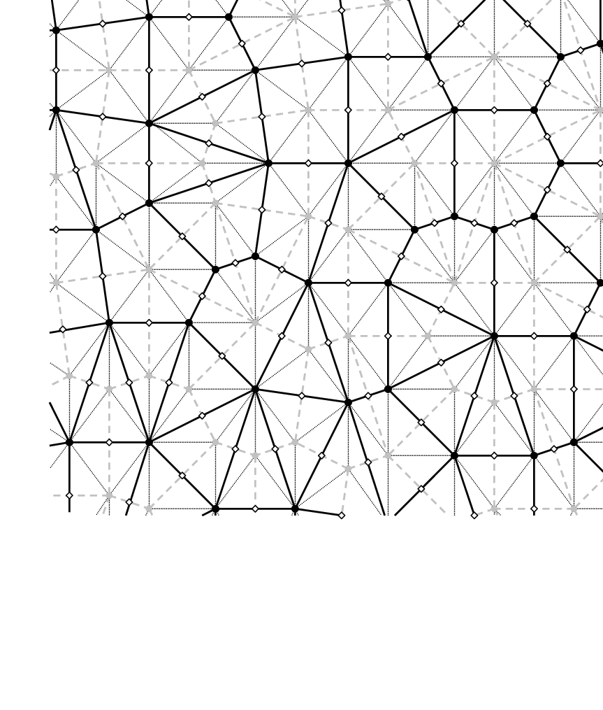
Throughout the paper, we work with isoradial graphs or, equivalently, rhombic lattices. A planar graph Γ\Gamma embedded in ℂ{\mathbb{C}} is called δ\delta-isoradial if each face is inscribed into a circle of a common radius δ\delta. If all circle centers are inside the corresponding faces, then one can naturally embed the dual graph Γ∗\Gamma^{*} in ℂ{\mathbb{C}} isoradially with the same δ\delta, taking the circle centers as vertices of Γ∗\Gamma^{*}. The name rhombic lattice is due to the fact that all quadrilateral faces of the corresponding bipartite graph Λ\Lambda (having Γ∪Γ∗\Gamma\cup\Gamma^{*} as vertices and radii of the circles as edges) are rhombi with sides of length δ\delta. We denote the set of rhombi centers by ♢\diamondsuit (example of an isoradial graph is drawn in Fig. 1A). We also require the following mild assumption:

the rhombi angles are uniformly bounded away from 00 and π\pi

(in other words, all these angles belong to [η,π−η][\eta,\pi\!-\!\eta] for some fixed η>0\eta>0). Below we often use the notation const for absolute positive constants that don’t depend on the mesh δ\delta or the graph structure but, in principle, may depend on η\eta. We also use the notation f≍gf\asymp g which means that a double-sided estimate const1⋅f⩽g⩽const2⋅g\mathop{\mathrm{const}}\nolimits_{1}\cdot f\leqslant g\leqslant\mathop{\mathrm{const}}\nolimits_{2}\cdot g holds true for some const1,2>0\mathop{\mathrm{const}}\nolimits_{1,2}>0 which are independent of δ\delta.

Refer to caption

(A)

Refer to caption

(B)

Refer to caption

(C)

Figure 1. (A) Example of an isoradial graph Γ\Gamma (black vertices, solid lines), its dual isoradial graph Γ∗\Gamma^{*} (gray vertices, dashed lines), the corresponding rhombic lattice or quad-graph (vertices Λ=Γ∪Γ∗\Lambda=\Gamma\cup\Gamma^{*}, thin lines) and the set ♢=Λ∗\diamondsuit=\Lambda^{*} (rhombi centers, white diamond-shaped vertices). (B) Local notation near u∈Γu\in\Gamma, with neighbors of uu enumerated counterclockwise by 1,2​…,s,s+1,…,n1,2\dots,s,s+1,\dots,n. The weight μΓδ​(u)\mu^{\delta}_{\Gamma}(u) is equal to the shaded polygon area. (C) Definition of s-holomorphic functions: F⁡(z0)F(z_{0}) and F⁡(z1)F(z_{1}) have the same projections on the direction [i⁡(w−u)]−12[i(w\!-\!u)]^{-\frac{1}{2}}. Thus, we have one real identity for each pair of neighboring z0z_{0}, z1z_{1}.

It is known that one can define the (critical) Ising model on Γ∗\Gamma^{*} so that

  1. (a)

    the interaction constants Jwi​wjJ_{w_{i}w_{j}} are local (namely, depend on the lengths of edges connecting wi,j∈Γ∗w_{i,j}\in\Gamma^{*}, wi∼wjw_{i}\sim w_{j}, only) and

  2. (b)

    the model is invariant under the star-triangle transform.

Such invariance is widely recognized as the crucial sign of the integrability. Note that the star-triangle transform preserves the isoradial graph/rhombic lattice structure. Moreover, isoradial graphs form the largest family of planar graphs (embedded into ℂ{\mathbb{C}}) satisfying these properties (see [CS06] and references therein). At the same time, discrete holomorphic functions on isoradial graphs provide the simplest example of a discrete integrable system in the so-called “consistency approach” to the (discrete) integrable systems theory (see [BS08]).

Recently, it was understood (see [Mer01, Smi06, RC06]) that some objects coming from the theoretical physics approach to the Ising model (namely, products of order and disorder operators with appropriate complex weights) can be considered and dealt with as discrete holomorphic functions (see Sect. 3.2 for further discussion). These functions (which we call basic observables or holomorphic fermions) provide a powerful tool for rigorous proofs of several results concerning the conformal invariance of the critical 2D Ising model. Implementing the program proposed and started in [Smi06, Smi07] for the square grid, in this paper we mainly focus our attention on the topologically simplest case, when the model is defined in the simply-connected (discrete) domain Ωδ\Omega^{\delta} having two marked boundary points aδ,bδa^{\delta},b^{\delta} (but see Section 6 for more involved setup). We have to mark some boundary points so that the conformal modulus is non-trivial, allowing us to construct conformal invariants.

We will work with two representations of the Ising model: the usual spin, as well as the random cluster (Fortuin-Kasteleyn). The observables are similar, but do not directly follow from each other, and require slightly different approaches. In either case there is an interface (between spin clusters or random clusters) – a discrete curve γδ\gamma^{\delta} running from aδa^{\delta} to bδb^{\delta} inside Ωδ\Omega^{\delta} (see Section 2.1, 2.2 for precise definitions). In both cases the basic observables are martingales with respect to (filtration induced by) the interface grown progressively from aδa^{\delta}, which opens the way to identify its scaling limit as a Schramm’s SLE curve, cf. [Smi06].

The interface in the random cluster representation can in principle pass through some point twice, but with our setup we move apart those passages, so that the curve becomes simple and when arriving at the intersection it is always clear how to proceed. This setup is unique where the martingale property holds, so there is only one conformally invariant way to address this problem. Note that the resulting scaling limit, the SLE⁡(16/3)\mathrm{SLE}(16/3) curve, will have double points. A similar ambiguity arises in the spin model (when, e.g. a vertex is surrounded by four spins “−+−+{-}{+}{-}{+}”), but regardless of the way to address it (e.g. deterministic, like always turning right, or probabilistic, like tossing a coin every time) the martingale property always holds, and so the SLE⁡(3)\mathrm{SLE}(3) is the scaling limit. The latter is almost surely simple, so we conclude that the double points in the discrete case produce only very small loops, disappearing in the scaling limit.

The first two results of our paper say that, in both representations, the holomorphic fermions are uniformly close to their continuous conformally invariant counterparts, independently of the structure of Γδ\Gamma^{\delta} (or ♢δ\diamondsuit^{\delta}) and the shape of Ωδ\Omega^{\delta} (in particular, we don’t use any smoothness assumptions concerning the boundary). Namely, we prove the following two theorems, formulated in detail as Theorems 4.3 and 5.6:

Theorem A (FK-Ising fermion).

Let discrete domains (Ωδ,aδ,bδ)(\Omega^{\delta};a^{\delta},b^{\delta}) with two marked boundary points aδ,bδa^{\delta},b^{\delta} approximate some continuous domain (Ω,a,b)(\Omega;a,b) as δ→0\delta\to 0. Then, uniformly on compact subsets of Ω\Omega and independently of the structure of ♢δ\diamondsuit^{\delta},

Fδ​(z)⇉Φ′​(z),F^{\delta}(z)\rightrightarrows\sqrt{\Phi^{\prime}(z)},

where Fδ​(z)=Fδ​(z,Ωδ,aδ,bδ)F^{\delta}(z)=F^{\delta}(z;\Omega^{\delta},a^{\delta},b^{\delta}) is the discrete holomorphic fermion and Φ\Phi denotes the conformal mapping from Ω\Omega onto the strip ℝ×(0,1){\mathbb{R}}\times(0,1) such that a,ba,b are mapped to ∓∞\mp\infty.

and

Theorem B (spin-Ising fermion).

Let discrete domains (Ωδ,aδ,bδ)(\Omega^{\delta};a^{\delta},b^{\delta}) approximate some continuous domain (Ω,a,b)(\Omega;a,b) as δ→0\delta\to 0. Then, uniformly on compact subsets of Ω\Omega and independently of the structure of Γδ\Gamma^{\delta},

Fδ​(z)⇉Ψ′​(z),F^{\delta}(z)\rightrightarrows\sqrt{\Psi^{\prime}(z)},

where Fδ=Fδ​(z,Ωδ,aδ,bδ)F^{\delta}=F^{\delta}(z;\Omega^{\delta},a^{\delta},b^{\delta}) is the discrete holomorphic fermion and Ψ:Ω→ℂ+\Psi:\Omega\to{\mathbb{C}}_{+} is the conformal mapping such that aa and bb are mapped to ∞\infty and 00, appropriately normalized at bb.

Because of the aforementioned martingale property, these results are sufficient to prove the convergence of interfaces to conformally invariant Schramm’s SLE curves (in our case, SLE⁡(3)\mathrm{SLE}(3) for the spin representation and SLE⁡(16/3)\mathrm{SLE}(16/3) for the FK representation) in the weak topology given by the convergence of driving forces in the Loewner equation, cf. [LSW04, Smi06]. A priori this is very far from establishing convergence of curve themselves, but we use techniques of [KS09] to prove this stronger convergence in [CS11, Smi11].

The third result shows how our techniques can be used to find the (conformally invariant) limit of some macroscopic quantities, “staying on the discrete level”, i.e. without consideration of the limiting curves. Namely, we prove a crossing probability formula for the critical FK-Ising model on isoradial graphs, analogous to Cardy’s formula [Smi01a, Smi01b] for critical percolation and formulated in detail as Theorem 6.1:

Theorem C (FK-Ising crossing probability).

Let discrete domains (Ωδ,aδ,bδ,cδ,dδ)(\Omega^{\delta};a^{\delta},b^{\delta},c^{\delta},d^{\delta}) with alternating (wired/free/wired/free) boundary conditions on four sides approximate some continuous topological quadrilateral (Ω,a,b,c,d)(\Omega;a,b,c,d) as δ→0\delta\to 0. Then the probability of an FK cluster crossing between two wired sides has a scaling limit, which depends only on the conformal modulus of the limiting quadrilateral, and is given for the half-plane by

p⁡(ℍ,0,−u,1,∞)=1−−u−u+−−u,u∈[0,1].p({\mathbb{H}};0,1\!-\!u,1,\infty)=\frac{\sqrt{1-\sqrt{1\!-\!u}}}{\sqrt{1\!-\!\sqrt{u}}+\sqrt{1\!-\!\sqrt{1\!-\!u}}}\,,~~u\in[0,1]. (1.1)

The version of this formula for multiple SLEs was derived by Bauer, Bernard and Kytölä in [BBK05], see page 1160, their notation for the modulus related to ours by x=1−ux=1-u. Besides being of an independent interest, this result together with [KS09] is needed to improve the topology of convergence of FK-Ising interfaces. Curiously, the (macroscopic) answer for a unit disc (𝔻,−ei​ϕ,e−i​ϕ,ei​ϕ,−e−i​ϕ)({\mathbb{D}};-e^{i\phi},e^{-i\phi},e^{i\phi},-e^{-i\phi}) formally coincides with the relative weights corresponding to two possible crossings inside (microscopic) rhombi (see Fig. 2A) in the critical model (see Remark 6.2).

1.3. Organization of the paper

We begin with the definition of Fortuin-Kasteleyn (random cluster) and spin representations of the critical Ising model on isoradial graphs in Section 2. From the outset we work with critical interactions, but in principle one can introduce a temperature parameter, which would lead to massive holomorphic fermions. We also introduce the basic discrete holomorphic observables (holomorphic fermions) satisfying the martingale property with respect to the growing interface and, essentially, show that they satisfy discrete version of the Cauchy-Riemann equation (Proposition 2.2 and Proposition 2.5) using some simple combinatorial bijections between the sets of configurations. Actually, we show that our observables satisfy the stronger “two-points” equation which we call spin or strong holomorphicity, or simply s-holomorphicity.

We discuss the properties of s-holomorphic functions in Section 3. The main results are:

  1. (a)

    The (rather miraculous) possibility to define naturally the discrete version of h⁡(z)=Im∫⁡(f⁡(z))2​𝑑zh(z)=\mathop{\mathrm{Im}}\nolimits\int(f(z))^{2}dz, see Proposition 3.6. Note that the square (f⁡(z))2(f(z))^{2} of a discrete holomorphic function f⁡(z)f(z) is not discrete holomorphic anymore, but unexpectedly it satisfies “half” of the Cauchy-Riemann equations, making its imaginary part a closed form with a well-defined integral;

  2. (b)

    The sub- and super-harmonicity of hh on the original isoradial graph Γ\Gamma and its dual Γ∗\Gamma^{*}, respectively, and the a priori comparability of the components h|Γh\big|_{\Gamma} and h|Γ∗h\big|_{\Gamma^{*}} which allows one to deal with hh as with a harmonic function: e.g. nonnegative hh’s satisfy a version of the Harnack Lemma (see Section 3.4);

  3. (c)

    The uniform (w.r.t. δ\delta and the structure of the isoradial graph/rhombic lattice Γ,Γ∗/♢\Gamma,\Gamma^{*}/\diamondsuit) boundedness and, moreover, uniform Lipschitzness of s-holomorphic functions inside their domains of definition Ωδ\Omega^{\delta}, with the constants depending on M=maxv∈Ωδ⁡|h⁡(v)|M=\max_{v\in\Omega^{\delta}}|h(v)| and the distance d=dist(z;∂Ωδ)d=\mathop{\mathrm{dist}}\nolimits(z;\partial\Omega^{\delta}) only (Theorem 3.12, these results should be considered as discrete analogous of the standard estimates from the classical complex analysis);

  4. (d)

    The combinatorial trick (see Section 3.6) that allows us to transform the discrete version of the Riemann-type boundary condition f⁡(ζ)|(τ⁡(ζ))−12f(\zeta)\parallel(\tau(\zeta))^{-\frac{1}{2}} into the Dirichlet condition for h|∂Ωh\big|_{\partial\Omega} on both Γ\Gamma and Γ∗\Gamma^{*}, thus completely avoiding the reference to Onsager’s magnetization estimate used in [Smi06, Smi07] to control the difference h|Γ−h|Γ∗h\big|_{\Gamma}-h\big|_{\Gamma^{*}} on the boundary.

We prove the (uniform) convergence of the basic observable in the FK-Ising model to its continuous counterpart in Section 4. The main result here is Theorem 4.3, which is the technically simplest of our main theorems, so the reader should consider the proof as a basic example of the application of our techniques. Besides the results from [CS08] and the previous Sections, the important idea (exactly as in [Smi07]) is to use some compactness arguments (in the set of all simply-connected domains equipped with the Carathéodory topology) in order to derive the uniform (w.r.t. to the shape of Ωδ\Omega^{\delta} and the structure of ♢δ\diamondsuit^{\delta}) convergence from the “pointwise” one.

In Section 5 we prove analogous convergence result for the holomorphic fermion defined for the spin representation of the critical Ising model (Theorem 5.6). There are two differences from the preceding Section: the unboundedness of the (discrete) integral h=Im∫⁡(f⁡(z))2​𝑑zh=\mathop{\mathrm{Im}}\nolimits\int(f(z))^{2}dz (this prevents us from the immediate use of compactness arguments) and the need to consider the normalization of our observable at the target point bδb^{\delta} (this is crucial for the martingale property). In order to handle the normalization at bδb^{\delta}, we assume that our domains Ωδ\Omega^{\delta} contain a (macroscopic) rectangle near bδb^{\delta} and their boundaries ∂Ωδ\partial\Omega^{\delta} approximate the corresponding straight segment as δ→0\delta\to 0. Making this technical assumption, we don’t lose much generality, since the growing interface, though fractal in the limit, doesn’t change the shape of the domain near bδb^{\delta}. Then, we use a version of the boundary Harnack principle (Proposition 5.3) in order to control the values of hh in the bulk through the fixed value f⁡(bδ)f(b^{\delta}). Another important technical ingredient is the universal (w.r.t. to the structure of ♢δ\diamondsuit^{\delta}) multiplicative normalization of our observable. Loosely speaking, we define it using the value at bδb^{\delta} of the discrete holomorphic fermion in the discrete half-plane (see Theorem 5.4 for further details).

Section 6 is devoted to the crossing probability formula for the FK-Ising model on discrete quadrilaterals (Ωδ,aδ,bδ,cδ,dδ)(\Omega^{\delta};a^{\delta},b^{\delta},c^{\delta},d^{\delta}) (Theorem 6.1, see also Remark 6.2). The main idea here is to construct some discrete holomorphic in Ωδ\Omega^{\delta} function whose boundary values reflect the conformal modulus of the quadrilateral. Namely, in our construction, discrete functions hδ=Im∫⁡(fδ​(z))2​𝑑zh^{\delta}=\mathop{\mathrm{Im}}\nolimits\int(f^{\delta}(z))^{2}dz approximate the imaginary part of the conformal mapping from Ωδ\Omega^{\delta} onto the slit strip [ℝ×(0,1)]∖(−∞+iϰ;iϰ][{\mathbb{R}}\times(0,1)]\setminus(-\infty+i\varkappa;i\varkappa] such that aδa^{\delta} is mapped to the “lower” −∞-\infty, bδb^{\delta} to +∞+\infty; cδc^{\delta} to the “upper” −∞-\infty and dδd^{\delta} to the tip i​ϰi\varkappa. The respective crossing probabilities are in the 11-to-11 correspondence with values ϰδ\varkappa^{\delta} which approximate ϰ\varkappa as δ→0\delta\to 0. Since ϰ\varkappa is uniquely determined by the limit of conformal moduli of (Ωδ,aδ,bδ,cδ,dδ)(\Omega^{\delta};a^{\delta},b^{\delta},c^{\delta},d^{\delta}), we obtain (1.1) (see further details in Section 6). Finally, Appendix contains several auxiliary lemmas: estimates of the discrete harmonic measure, discrete version of the Cauchy formula, and technical estimates of the Green function in the disc. We refer the reader interested in a more detailed presentation of the discrete complex analysis on isoradial graphs to our paper [CS08].

Acknowledgments. This research was supported by the Swiss N.S.F., by the European Research Council AG CONFRA, and by the Chebyshev Laboratory (Department of Mathematics and Mechanics, Saint-Petersburg State University) under the grant 11.G34.31.0026 of the Government of the Russian Federation. The first author was partially funded by P.Deligne’s 2004 Balzan prize in Mathematics and by the grant MK-7656.2010.1.

2. Critical spin- and FK-Ising models on isoradial graphs.
Basic observables (holomorphic fermions)

2.1. Critical FK-Ising model

2.1.1. Loop representation of the model, holomorphic fermion, martingale property

Refer to caption

θconfig.​(z)=θ\theta_{\mathrm{config.}}(z)=\theta,

relative weight =sin⁡12​θ=~\sin\tfrac{1}{2}\theta

Refer to caption

θconfig.​(z)=θ∗=π2−θ\theta_{\mathrm{config.}}(z)=\theta^{*}=\tfrac{\pi}{2}-\theta,

relative weight =sin⁡12​θ∗=~\sin\tfrac{1}{2}\theta^{*}

(A)

Refer to caption

(B)

Figure 2. (A) Loop representation of the critical FK-Ising model on isoradial graphs: the relative weights corresponding to two possible choices of connections inside the inner rhombus zz (the partition function is given by (2.2)). (B) Discrete domain Ω♢δ\Omega^{\delta}_{\diamondsuit} with a sample configuration. Besides loops, there is an interface γδ\gamma^{\delta} connecting aδa^{\delta} to bδb^{\delta}. Calculating the winding(γδ;bδ↝ξ)\mathop{\mathrm{winding}}\nolimits(\gamma^{\delta};\,b^{\delta}\rightsquigarrow\xi), we draw γδ\gamma^{\delta} so that it intersects the edge ξ=[ξb​ξw]\xi=[\xi_{\mathrm{b}}\xi_{\mathrm{w}}] orthogonally. As γδ\gamma^{\delta} grows, it separates some part of Ω♢δ\Omega^{\delta}_{\diamondsuit} (shaded) from bδb^{\delta}. We denote by Ω♢δ∖[aδγ1δ..γjδ]\Omega^{\delta}_{\diamondsuit}\setminus[a^{\delta}\gamma^{\delta}_{1}..\gamma^{\delta}_{j}] the connected component containing bδb^{\delta} (unshaded).

We will work with a graph domain which can be thought of as a discretization of a simply-connected planar domain with two marked boundary points. Let Ω♢δ⊂♢\Omega^{\delta}_{\diamondsuit}\!\subset\!\diamondsuit be a simply-connected discrete domain composed of inner rhombi z∈IntΩ♢δz\!\in\!\mathop{\mathrm{Int}}\nolimits\Omega^{\delta}_{\diamondsuit} and boundary half-rhombi ζ∈∂Ω♢δ\zeta\in\partial\Omega^{\delta}_{\diamondsuit}, with two marked boundary points aδa^{\delta}, bδb^{\delta} and Dobrushin boundary conditions (see Fig. 2B): ∂Ω♢δ\partial\Omega^{\delta}_{\diamondsuit} consists of the “white” arc awδ​bwδa^{\delta}_{\mathrm{w}}b^{\delta}_{\mathrm{w}}, the “black” arc bbδ​abδb^{\delta}_{\mathrm{b}}a^{\delta}_{\mathrm{b}}, and two edges [abδ​awδ][a^{\delta}_{\mathrm{b}}a^{\delta}_{\mathrm{w}}], [bbδ​bwδ][b^{\delta}_{\mathrm{b}}b^{\delta}_{\mathrm{w}}] of Λ\Lambda. Without loss of generality, we assume that

bbδ−bwδ=i​δb^{\delta}_{\mathrm{b}}-b^{\delta}_{\mathrm{w}}=i\delta, i.e., the edge bδ=[bbδ​bwδ]b^{\delta}=[b^{\delta}_{\mathrm{b}}b^{\delta}_{\mathrm{w}}] is oriented vertically.

For each inner rhombus z∈IntΩ♢δz\in\mathop{\mathrm{Int}}\nolimits\Omega^{\delta}_{\diamondsuit} we choose one of two possibilities to connect its sides (see Fig. 2A, there is only one choice for boundary half-rhombi), thus obtaining the set of configurations (whose cardinality is 2#⁡(IntΩ♢δ)2^{\mathrm{\#(\mathop{\mathrm{Int}}\nolimits\Omega^{\delta}_{\diamondsuit})}}). The partition function of the critical FK-Ising model is given by

Z=∑config.2#⁡(loops)​∏z∈IntΩ♢δsin⁡12​θconfig.​(z),Z=\sum_{\mathrm{config.}}~{\textstyle\sqrt{2}^{\,\mathrm{\#(loops)}}\prod_{z\in\mathop{\mathrm{Int}}\nolimits\Omega^{\delta}_{\diamondsuit}}\sin\frac{1}{2}\theta_{\mathrm{config.}}(z)}, (2.2)

where θconfig.​(z)\theta_{\mathrm{config.}}(z) is equal to either θ\theta or θ∗=π2−θ\theta^{*}=\frac{\pi}{2}-\theta depending on the choice of connections inside rhombus zz (see Fig. 2A).

We described the loop representation, since at criticality it is easier to work with, than the usual random cluster one. The loops trace the perimeters of random clusters, and the curve joining the two marked boundary points is the interface between a cluster and a dual cluster wired on two opposite boundary arcs (the so-called Dobrushin boundary conditions).

Let ξ=[ξb​ξw]\xi=[\xi_{\mathrm{b}}\xi_{\mathrm{w}}] be some inner edge of Ω♢δ\Omega^{\delta}_{\diamondsuit} (where ξb∈Γ\xi_{\mathrm{b}}\in\Gamma, ξw∈Γ∗\xi_{\mathrm{w}}\in\Gamma^{*}). Due to the boundary conditions chosen, each configuration consists of (a number of) loops and one interface γδ\gamma^{\delta} running from aδa^{\delta} to bδb^{\delta}. The holomorphic fermion is defined as

Fδ(ξ)=F(Ωδ,aδ,bδ)δ(ξ):=(2δ)−12⋅𝔼[χ(ξ∈γδ)⋅e−i2winding(γδ;bδ↝ξ)],F^{\delta}(\xi)=F^{\delta}_{(\Omega^{\delta};\,a^{\delta},b^{\delta})}(\xi):=(2\delta)^{-\frac{1}{2}}\cdot{\mathbb{E}}\left[\,\chi(\xi\!\in\!\gamma^{\delta})\cdot e^{-\frac{i}{2}\mathop{\mathrm{winding}}\nolimits(\gamma^{\delta};\,b^{\delta}\rightsquigarrow\xi)}\,\right], (2.3)

where χ⁡(ξ∈γδ)\chi(\xi\!\in\!\gamma^{\delta}) is the indicator function of the event that the interface intersects ξ\xi and

winding(γδ;bδ↝ξ)=winding(γδ;aδ↝ξ)−winding(γδ;aδ↝bδ)\mathop{\mathrm{winding}}\nolimits(\gamma^{\delta};\,b^{\delta}\rightsquigarrow\xi)=\mathop{\mathrm{winding}}\nolimits(\gamma^{\delta};\,a^{\delta}\rightsquigarrow\xi)-\mathop{\mathrm{winding}}\nolimits(\gamma^{\delta};\,a^{\delta}\rightsquigarrow b^{\delta}) (2.4)

denotes the total turn of γδ\gamma^{\delta} measured (in radians) from bδb^{\delta} to ξ\xi. Note that, for all configurations and edges ξ\xi one has (see Fig. 2B),

e−i2winding(γδ;bδ↝ξ)∥[i(ξw−ξb)]−12.e^{-\frac{i}{2}\mathop{\mathrm{winding}}\nolimits(\gamma^{\delta};\,b^{\delta}\rightsquigarrow\xi)}~\parallel\ [i(\xi_{\mathrm{w}}\!-\!\xi_{\mathrm{b}})]^{-\frac{1}{2}}\,.
Remark 2.1 (Martingale property).

For each ξ\xi, F(Ωδ∖[aδγδ1..γδj];γδj,bδ)δ(ξ)F^{\delta}_{(\Omega^{\delta}\setminus[a^{\delta}\gamma^{\delta}_{1}..\gamma^{\delta}_{j}];\gamma^{\delta}_{j},b^{\delta})}(\xi) is a martingale with respect to the growing interface (aδ=γ0δ,γ1δ,…,γjδ,…)(a^{\delta}=\gamma^{\delta}_{0},\gamma^{\delta}_{1},...,\gamma^{\delta}_{j},...) (till the stopping time when γδ\gamma^{\delta} hits ξ\xi or ξ\xi becomes separated from bδb^{\delta} by the interface, see Fig. 2B).

Proof.

Since the winding(γδ;bδ↝ξ)\mathop{\mathrm{winding}}\nolimits(\gamma^{\delta};\,b^{\delta}\rightsquigarrow\xi) doesn’t depend on the beginning of the interface, the claim immediately follows from the total probability formula. ∎

2.1.2. Discrete boundary value problem for FδF^{\delta}.

We start with the extension of FδF^{\delta} to the centers of rhombi z∈Ω♢δz\in\Omega^{\delta}_{\diamondsuit}. Actually, the (rather fortunate) opportunity to use the definition given below reflects the discrete holomorphicity of FδF^{\delta} (see discussion in Section 3.2).

Proposition 2.2.

Let z∈IntΩ♢δz\in\mathop{\mathrm{Int}}\nolimits\Omega^{\delta}_{\diamondsuit} be the center of some inner rhombus u1​w1​u2​w2u_{1}w_{1}u_{2}w_{2}. Then, there exists a complex number Fδ​(z)F^{\delta}(z) such that

Fδ​([uj​wk])=Proj⁡[Fδ​(z);[i⁡(wk−uj)]−12],j,k=1,2.F^{\delta}([u_{j}w_{k}])=\mathrm{Proj}\left[\,F^{\delta}(z)\,;\,[i(w_{k}\!-\!u_{j})]^{-\frac{1}{2}}\right],\quad j,k=1,2. (2.5)

The proposition essentially states that FδF^{\delta} is spin holomorphic as specified in Definition 3.1 below. By Proj⁡[X;u]\mathrm{Proj}[X;u] we denote the orthogonal projection of the vector XX on the vector uu, which is parallel to uu and equal to

Proj⁡[X;u]=Re(X​u¯|u|)​u|u|=X2+X¯​u22​|u|2\mathrm{Proj}[X;u]=\mathop{\mathrm{Re}}\nolimits\biggl(X\frac{\overline{u}}{|u|}\biggr)\frac{u}{|u|}=\frac{X}{2}+\frac{\overline{X}u^{2}}{2|u|^{2}}

(here we consider complex numbers as vectors). Because of the latter rewriting, the choice of the sign in the square root in (2.5) does not matter.

Refer to caption
Figure 3. Local rearrangement at zz: the bijection between configurations. Without loss of generality, we may assume that the (reversed, i.e., going from bδb^{\delta}) interface enters the rhombus zz through the edge [u2​w1][u_{2}w_{1}] (the case [u1​w2][u_{1}w_{2}] is completely similar). There are two possibilities: either γδ\gamma^{\delta} (finally) leaves zz through [u1​w1][u_{1}w_{1}] (“L”, left turn) or through [u2​w2][u_{2}w_{2}] (“R”, right turn). In view of (2.2), the relative weights of configurations are 2​sin⁡12​θ\sqrt{2}\sin\tfrac{1}{2}\theta, sin⁡12​θ∗\sin\tfrac{1}{2}\theta^{*} (“L” pairs), and sin⁡12​θ\sin\tfrac{1}{2}\theta, 2​sin⁡12​θ∗\sqrt{2}\sin\tfrac{1}{2}\theta^{*} (“R” pairs).
Proof.

As on the square grid (see [Smi07]), the proof is based on the bijection between configurations which is produced by their local rearrangement at zz. It is sufficient to check that the contributions to Fδ​([uj​wk])F^{\delta}([u_{j}w_{k}])’s of each pair of configurations drawn in Fig. 3 are the specified projections of the same complex number. The relative contributions of configurations (up to the same real factor coming from the structure of the configuration away from zz) to the values of FF on four edges around zz for the pairs “L” and “R” are given by

ei​φ2⋅Fδ​([u2​w1])e^{i\frac{\varphi}{2}}\!\cdot F^{\delta}([u_{2}w_{1}]) ei​φ2⋅Fδ​([u2​w2])e^{i\frac{\varphi}{2}}\!\cdot F^{\delta}([u_{2}w_{2}]) ei​φ2⋅Fδ​([u1​w2])e^{i\frac{\varphi}{2}}\!\cdot F^{\delta}([u_{1}w_{2}]) ei​φ2⋅Fδ​([u1​w1])e^{i\frac{\varphi}{2}}\!\cdot F^{\delta}([u_{1}w_{1}])
L\vphantom{\big|^{|}_{|}}\mathrm{L} 2​sin⁡θ2+sin⁡θ∗2\sqrt{2}\sin\frac{\theta}{2}+\sin\frac{\theta^{*}}{2} ei​θ​sin⁡θ∗2e^{i\theta}\sin\frac{\theta^{*}}{2} −i​sin⁡θ∗2-i\sin\frac{\theta^{*}}{2} e−i​θ∗​[2​sin⁡θ2+sin⁡θ∗2]e^{-i\theta^{*}}[\sqrt{2}\sin\frac{\theta}{2}+\sin\frac{\theta^{*}}{2}]
R\vphantom{\big|^{|}_{|}}\mathrm{R} sin⁡θ2+2​sin⁡θ∗2\sin\frac{\theta}{2}+\sqrt{2}\sin\frac{\theta^{*}}{2} ei​θ​[sin⁡θ2+2​sin⁡θ∗2]e^{i\theta}[\sin\frac{\theta}{2}+\sqrt{2}\sin\frac{\theta^{*}}{2}] i​sin⁡θ2i\sin\frac{\theta}{2} e−i​θ∗​sin⁡θ2e^{-i\theta^{*}}\sin\frac{\theta}{2}

where φ\varphi denotes the total turn of the interface traced from bδb^{\delta} to [u2​w1][u_{2}w_{1}]. An easy trigonometric calculation using that θ+θ∗=π/2\theta+\theta^{*}=\pi/2 shows that

[2​sin⁡θ2+sin⁡θ∗2]−i​sin⁡θ∗2=ei​θ​sin⁡θ∗2+e−i​θ∗​[2​sin⁡θ2+sin⁡θ∗2].\textstyle\left[\sqrt{2}\sin\frac{\theta}{2}+\sin\frac{\theta^{*}}{2}\right]~-~i\sin\frac{\theta^{*}}{2}~=~e^{i\theta}\sin\frac{\theta^{*}}{2}~+~e^{-i\theta^{*}}\left[\sqrt{2}\sin\frac{\theta}{2}+\sin\frac{\theta^{*}}{2}\right]~.

Denoting the common value of the two sides by ei​φ2⋅Fδ​(z)e^{i\frac{\varphi}{2}}\cdot F^{\delta}(z) and observing that 1⟂i1\perp i and ei​θ⟂e−i​θ∗e^{i\theta}\perp e^{-i\theta^{*}}, we conclude that the first row (“L”) describes the four projections of ei​φ2⋅Fδ​(z)e^{i\frac{\varphi}{2}}\cdot F^{\delta}(z) onto the lines ℝ{\mathbb{R}}, ei​θ​ℝe^{i\theta}{\mathbb{R}}, i​ℝi{\mathbb{R}} and e−i​θ∗​ℝe^{-i\theta^{*}}{\mathbb{R}}, respectively. Multiplying by the common factor e−i​φ2e^{-i\frac{\varphi}{2}} (which is always parallel to [i⁡(w1−u2)]−12[i(w_{1}\!-\!u_{2})]^{-\frac{1}{2}}), we obtain the result for “L” pairs of configurations. The interchanging of θ\theta and θ∗\theta^{*} yields the result for “R” pairs. ∎

Remark 2.3.

For ζ∈∂Ω♢δ\zeta\in\partial\Omega^{\delta}_{\diamondsuit} we define Fδ​(ζ)F^{\delta}(\zeta) so that (2.5) holds true (in this case, only two projections are meaningful, so Fδ​(ζ)F^{\delta}(\zeta) is easily and uniquely defined). Note that all interfaces passing through the half-rhombus ζ\zeta intersect both its sides. Moreover, since the winding of the interface at ζ\zeta is independent of the configuration chosen (and coincides with the winding of the corresponding boundary arc) for topological reasons, we have

Fδ​(ζ)|(τ⁡(ζ))−12,ζ∈∂Ω♢δ,F^{\delta}(\zeta)\parallel(\tau(\zeta))^{-\frac{1}{2}},\quad\zeta\in\partial\Omega^{\delta}_{\diamondsuit}, (2.6)

where (see Fig. 2B)

τ⁡(ζ)=w2​(ζ)−w1​(ζ),ζ∈(aδ​bδ),w1,2​(ζ)∈Γ∗,τ⁡(ζ)=u2​(ζ)−u1​(ζ),ζ∈(bδ​aδ),u1,2​(ζ)∈Γ,\begin{array}[]{lll}\tau(\zeta)=w_{2}(\zeta)\!-\!w_{1}(\zeta),&\zeta\in(a^{\delta}b^{\delta}),&w_{1,2}(\zeta)\in\Gamma^{*},\cr\tau(\zeta)=u_{2}(\zeta)\!-\!u_{1}(\zeta),&\zeta\in(b^{\delta}a^{\delta}),&u_{1,2}(\zeta)\in\Gamma,\end{array}

is the “ discrete tangent vector” to ∂Ω♢δ\partial\Omega^{\delta}_{\diamondsuit} directed from aδa^{\delta} to bδb^{\delta} on both boundary arcs.

Thus, we arrive at

Discrete Riemann boundary value problem for Fδ\bm{F^{\delta}} (FK-case): The function FδF^{\delta} is defined in Ω♢δ\Omega^{\delta}_{\diamondsuit} and for each pair of neighbors z0,z1∈Ω♢δz_{0},z_{1}\in\Omega^{\delta}_{\diamondsuit}, z0∼z1z_{0}\sim z_{1}, the discrete holomorphicity condition holds:

Proj⁡[Fδ​(z0);[i⁡(w−u)]−12]=Proj⁡[Fδ​(z1);[i⁡(w−u)]−12].\mathrm{Proj}\left[F^{\delta}(z_{0})\,;[i(w\!-\!u)]^{-\frac{1}{2}}\right]=\mathrm{Proj}\left[F^{\delta}(z_{1})\,;[i(w\!-\!u)]^{-\frac{1}{2}}\right]. (2.7)

Moreover, FδF^{\delta} satisfies the boundary conditions (2.6) and, since all interfaces pass through bδb^{\delta}, satisfies the normalization Fδ​(bδ)=ReFδ​(b♢δ)=(2​δ)−12F^{\delta}(b^{\delta})=\mathop{\mathrm{Re}}\nolimits F^{\delta}(b^{\delta}_{\diamondsuit})=(2\delta)^{-\frac{1}{2}}.

2.2. Critical spin-Ising model

2.2.1. Definition of the model, holomorphic fermion, martingale property

Refer to caption

(A)

Refer to caption

(B)

Figure 4. (A) Ising model on isoradial graphs: discrete domain Ω♢δ\Omega^{\delta}_{\diamondsuit} and a sample configuration (the partition function is given by (2.8)). By our choice of the “turning rule,” loops and the interface γδ\gamma^{\delta} separate clusters of “++” spins connected through edges and clusters of “−-” spins connected through vertices. To illustrate this, γδ\gamma^{\delta} and loops are drawn slightly closer to “++” spins. The component of Ωδ\Omega^{\delta} not “swallowed” by the path [aδγ1δ..γjδ][a^{\delta}\gamma^{\delta}_{1}..\gamma^{\delta}_{j}] is unshaded. The vertex u1u_{1} is shaded since it is not connected to bδb^{\delta} anymore. The vertices u2u_{2} and u3u_{3} are shaded too since each of them is connected to the bulk by a single edge which contradicts our definition of connected discrete domains. Moreover, since the “interface” aδ↝γjδ↝za^{\delta}\rightsquigarrow\gamma_{j}^{\delta}\rightsquigarrow z could arrive at each of these points only in a single way, our observable certainly satisfies boundary condition (2.11) at z2z_{2} and z3z_{3}, thus not distinguishing them from the other boundary points. (B) Two samples of “interface pictures” composed from a number of loops and a single interface γδ\gamma^{\delta} running from aδa^{\delta} to zz. To define the winding(γδ;aδ↝z)\mathop{\mathrm{winding}}\nolimits(\gamma^{\delta};\,a^{\delta}\rightsquigarrow z) unambiguously, we draw γδ\gamma^{\delta} so that, if there is a choice, it turns to the left (for z∈∂Ω♢δz\in\partial\Omega^{\delta}_{\diamondsuit}, this corresponds to the edge-connectivity of “++” clusters).

Let Ω♢δ⊂♢\Omega^{\delta}_{\diamondsuit}\!\subset\!\diamondsuit be a simply-connected discrete domain composed of inner rhombi z∈IntΩ♢δz\!\in\!\mathop{\mathrm{Int}}\nolimits\Omega^{\delta}_{\diamondsuit} and boundary half-rhombi ζ∈∂Ω♢δ\zeta\in\partial\Omega^{\delta}_{\diamondsuit}, with two marked boundary points aδ,bδ∈∂Ω♢δa^{\delta},b^{\delta}\in\partial\Omega^{\delta}_{\diamondsuit}, such that ∂Ω♢δ\partial\Omega^{\delta}_{\diamondsuit} contains only “white” vertices (see Fig. 4A) and there is no edge of Γ∗\Gamma^{*} breaking Ω♢δ\Omega^{\delta}_{\diamondsuit} into two non-connected pieces.

To each inner “white” vertex w∈IntΩΓ∗δw\in\mathop{\mathrm{Int}}\nolimits\Omega^{\delta}_{\Gamma^{*}}, we assign the spin σ⁡(w)\sigma(w) (++ or −-), thus obtaining the set of configurations (whose cardinality is 2#⁡(IntΩΓ∗δ)2^{\mathrm{\#(\mathop{\mathrm{Int}}\nolimits\Omega^{\delta}_{\Gamma^{*}})}}). We also impose Dobrushin boundary conditions assigning the −- spins to vertices on the boundary arc (aδ​bδ)(a^{\delta}b^{\delta}) and the ++ spins on the boundary arc (bδ​aδ)(b^{\delta}a^{\delta}) (see Fig. 4A). The partition function of the critical spin-Ising model is given by

Z~(Ωδ;aδ↝bδ)=[sin12θ(bδ)]−1∑spin​config.∏w1∼w2:σ⁡(w1)≠σ⁡(w2)xw1​w2,xw1​w2=tan12θ(z),\widetilde{Z}_{(\Omega^{\delta};\,a^{\delta}\rightsquigarrow b^{\delta})}=[\sin\tfrac{1}{2}\theta(b^{\delta})]^{-1}\!\!\!\!\sum_{\mathrm{spin~config.}}~{\textstyle\prod_{w_{1}\sim w_{2}:\sigma(w_{1})\neq\sigma(w_{2})}x_{w_{1}w_{2}},\quad x_{w_{1}w_{2}}=\tan\frac{1}{2}\theta(z)}, (2.8)

where θ⁡(z)\theta(z) is the half-angle of the rhombus u1​w1​u2​w2u_{1}w_{1}u_{2}w_{2} having center at zz (i.e., tan⁡θw1​w2=|w2−w1|/|u2−u1|\tan\theta_{w_{1}w_{2}}\!=|w_{2}-w_{1}|/|u_{2}-u_{1}|). The first factor sin−1\sin^{-1} doesn’t depend on the configuration, and is introduced for technical reasons.

Due to Dobrushin boundary conditions, for each configuration, there is an interface γδ\gamma^{\delta} running from aδa^{\delta} to bδb^{\delta} and separating ++ spins from −- spins. If Γ\Gamma is not a trivalent graph, one needs to specify the algorithm of “extracting γδ\gamma^{\delta} from the picture”, if it can be done in different ways. Below we assume that,

if there is a choice, the “interface” takes the left-most possible route (see Fig. 4).

With this choice the interface separates clusters of “++” spins connected through edges and clusters of “−-” spins connected through vertices. Any other choice would do for the martingale property and eventual conformal invariance, as discussed in the Introduction. For example, one can toss a coin at each vertex to decide whether “++” or “−-” spin clusters connect through it. Note that, drawing all the edges separating ++ spins from −- spins, one can rewrite the partition function as a sum over all configurations ϖ\varpi of edges which consist of a single interface running from aδa^{\delta} to bδb^{\delta} and a number of loops. Namely,

Z~(Ωδ;aδ↝bδ)=[sin12θ(bδ)]−1∑ϖ={interface+loops}∏w1∼w2:[w1;w2]​intersects​ωxw1​w2.\widetilde{Z}_{(\Omega^{\delta};\,a^{\delta}\rightsquigarrow b^{\delta})}=[\sin\tfrac{1}{2}\theta(b^{\delta})]^{-1}\!\!\!\!\!\!\sum_{\varpi=\{\mathrm{interface}+\mathrm{loops}\}}~{\textstyle\prod_{w_{1}\sim w_{2}:[w_{1};w_{2}]~\mathrm{intersects}~\omega}x_{w_{1}w_{2}}}\,. (2.9)

For z∈Ω♢δz\in\Omega^{\delta}_{\diamondsuit}, the holomorphic fermion is defined as (cf. (2.3), (2.4))

Fδ​(z)=F(Ωδ,aδ,bδ)δ​(z):=ℱδ​(bδ)⋅Z~(Ωδ;aδ↝z)⋅𝔼(Ωδ;aδ↝z)e−i2winding(γδ;aδ↝z)Z~(Ωδ;aδ↝bδ)⋅e−i2winding(aδ↝bδ).F^{\delta}(z)=F^{\delta}_{(\Omega^{\delta};\,a^{\delta},b^{\delta})}(z):={\mathcal{F}}^{\delta}(b^{\delta})\cdot\frac{\widetilde{Z}_{(\Omega^{\delta};\,a^{\delta}\rightsquigarrow z)}\cdot{\mathbb{E}}_{(\Omega^{\delta};\,a^{\delta}\rightsquigarrow z)}e^{-\frac{i}{2}\mathop{\mathrm{winding}}\nolimits(\gamma^{\delta};\,a^{\delta}\rightsquigarrow z)}}{\widetilde{Z}_{(\Omega^{\delta};\,a^{\delta}\rightsquigarrow b^{\delta})}\cdot e^{-\frac{i}{2}\mathop{\mathrm{winding}}\nolimits(a^{\delta}\rightsquigarrow b^{\delta})}}\,. (2.10)

As in (2.9), Z~(Ωδ;aδ↝zδ)\widetilde{Z}_{(\Omega^{\delta};\,a^{\delta}\rightsquigarrow z^{\delta})} denotes the partition function for the set of “interfaces pictures” containing (besides loops) one interface γδ\gamma^{\delta} running from aδa^{\delta} to zz (see Fig. 4B),

for each configuration we count all weights corresponding to the drawn edges, including tan⁡12​θ​(aδ)\tan\tfrac{1}{2}\theta(a^{\delta}) and [cos⁡12​θ​(z)]−1=[sin⁡12​θ​(z)]−1⋅tan⁡12​θ​(z)[\cos\frac{1}{2}\theta(z)]^{-1}=[\sin\frac{1}{2}\theta(z)]^{-1}\cdot\tan\frac{1}{2}\theta(z) for the first and the last.

Then 𝔼(Ωδ;aδ↝zδ){\mathbb{E}}_{(\Omega^{\delta};\,a^{\delta}\rightsquigarrow z^{\delta})} will stand for the expectation with respect to the corresponding probability measure. Equivalently, one can take the partition function, multiplying the weight of each configuration by the complex factor e−i2winding(γδ;aδ↝zδ)e^{-\frac{i}{2}\mathop{\mathrm{winding}}\nolimits(\gamma^{\delta};\,a^{\delta}\rightsquigarrow z^{\delta})} (which, for z∈IntΩ♢δz\in\mathop{\mathrm{Int}}\nolimits\Omega^{\delta}_{\diamondsuit}, may be equal to one of the four different complex values α\alpha, i​αi\alpha, −α-\alpha, −i​α-i\alpha depending on the particular configuration). Finally,

ℱδ(bδ)∥(τ(bδ))−1/2{\mathcal{F}}^{\delta}(b^{\delta})\parallel(\tau(b^{\delta}))^{-1/2}, where τ⁡(bδ)=w2​(bδ)−w1​(bδ)\tau(b^{\delta})=w_{2}(b^{\delta})\!-\!w_{1}(b^{\delta}), is a normalizing factor that depends only on the structure of ♢δ\diamondsuit^{\delta} near bδb^{\delta} (see Section 5.1).

Here and below, for ζ∈∂Ω♢δ\zeta\in\partial\Omega^{\delta}_{\diamondsuit}, τ⁡(ζ)=w2​(ζ)−w1​(ζ)\tau(\zeta)=w_{2}(\zeta)\!-\!w_{1}(\zeta) denotes “discrete tangent vector” to ∂Ω♢δ\partial\Omega^{\delta}_{\diamondsuit} oriented counterclockwise (see Fig. 4A for notation). For any ζ∈∂Ω♢δ\zeta\in\partial\Omega^{\delta}_{\diamondsuit}, the winding(γδ;aδ↝ζ)\mathop{\mathrm{winding}}\nolimits(\gamma^{\delta};\,a^{\delta}\rightsquigarrow\zeta) is fixed due to topological reasons, and so

Fδ​(ζ)|(τ⁡(ζ))−12,ζ∈∂Ω♢δ∖{aδ},𝑤ℎ𝑖𝑙𝑒Fδ​(aδ)|i​(τ⁡(aδ))−12.F^{\delta}(\zeta)\parallel(\tau(\zeta))^{-\frac{1}{2}},\quad\zeta\in\partial\Omega^{\delta}_{\diamondsuit}\setminus\{a^{\delta}\},\quad\mathit{while}\quad F^{\delta}(a^{\delta})\parallel i(\tau(a^{\delta}))^{-\frac{1}{2}}. (2.11)
Remark 2.4 (Martingale property).

For each z∈IntΩ♢δz\in\mathop{\mathrm{Int}}\nolimits\Omega^{\delta}_{\diamondsuit}, F(Ωδ∖[aδ​γjδ],γjδ,bδ)δ​(z)F^{\delta}_{(\Omega^{\delta}\setminus[a^{\delta}\gamma^{\delta}_{j}];\gamma^{\delta}_{j},b^{\delta})}(z) is a martingale with respect to the growing interface (aδ=γ0δ,γ1δ,…,γjδ,…)(a^{\delta}=\gamma^{\delta}_{0},\gamma^{\delta}_{1},...,\gamma^{\delta}_{j},...) (till the stopping time when γδ\gamma^{\delta} hits ξ\xi or zz becomes separated from bδb^{\delta} by the interface, see Fig. 4A).

Proof.

It is sufficient to check that FδF^{\delta} has the martingale property when γδ\gamma^{\delta} makes one step. Let aLδ,..,aRδa^{\delta}_{\mathrm{L}},..,a^{\delta}_{\mathrm{R}} denote all possibilities for the first step. Then,

Z~(Ωδ;aδ↝bδ)=tan12θ(aδ)⋅[Z~(Ωδ∖[aδaδL];aδL↝bδ)+…+Z~(Ωδ∖[aδaδR];aδR↝bδ)],\widetilde{Z}_{(\Omega^{\delta};\,a^{\delta}\rightsquigarrow b^{\delta})}=\tan\tfrac{1}{2}\theta(a^{\delta})\cdot\left[\widetilde{Z}_{(\Omega^{\delta}\setminus[a^{\delta}a^{\delta}_{\mathrm{L}}];\,a^{\delta}_{\mathrm{L}}\rightsquigarrow b^{\delta})}+...+\widetilde{Z}_{(\Omega^{\delta}\setminus[a^{\delta}a^{\delta}_{\mathrm{R}}];\,a^{\delta}_{\mathrm{R}}\rightsquigarrow b^{\delta})}\right], (2.12)

and so

ℙ⁡(γ1δ=aLδ)=Z~(Ωδ∖[aδaδL];aδL↝bδ)[tan12θ(aδ)]−1Z~(Ωδ;aδ↝bδ),…,ℙ⁡(γ1δ=aRδ)=Z~(Ωδ∖[aδaδR];aδR↝bδ)[tan12θ(aδ)]−1Z~(Ωδ;aδ↝bδ).{{\mathbb{P}}(\gamma^{\delta}_{1}\!=\!a^{\delta}_{\mathrm{L}})}=\frac{\widetilde{Z}_{(\Omega^{\delta}\setminus[a^{\delta}a^{\delta}_{\mathrm{L}}];\,a^{\delta}_{\mathrm{L}}\rightsquigarrow b^{\delta})}}{[{\tan\tfrac{1}{2}\theta(a^{\delta})}]^{-1}\widetilde{Z}_{(\Omega^{\delta};\,a^{\delta}\rightsquigarrow b^{\delta})}}~,~\dots\ ,~{{\mathbb{P}}(\gamma^{\delta}_{1}\!=\!a^{\delta}_{\mathrm{R}})}=\frac{\widetilde{Z}_{(\Omega^{\delta}\setminus[a^{\delta}a^{\delta}_{\mathrm{R}}];\,a^{\delta}_{\mathrm{R}}\rightsquigarrow b^{\delta})}}{[{\tan\tfrac{1}{2}\theta(a^{\delta})}]^{-1}\widetilde{Z}_{(\Omega^{\delta};\,a^{\delta}\rightsquigarrow b^{\delta})}}\,.

Taking into account that the difference

winding(aδ↝bδ)−winding(aLδ↝bδ)=winding(aδ→aLδ),\mathop{\mathrm{winding}}\nolimits(a^{\delta}\rightsquigarrow b^{\delta})-\mathop{\mathrm{winding}}\nolimits(a^{\delta}_{\mathrm{L}}\rightsquigarrow b^{\delta})=\mathop{\mathrm{winding}}\nolimits(a^{\delta}\to a^{\delta}_{\mathrm{L}}),

we obtain

ℙ⁡(γ1δ=aLδ)⋅F(Ωδ∖[aδ​aLδ],aLδ,b)δ​(z)F(Ωδ,aδ,b)δ​(z)=e−i2winding(aδ→aδL)[tan⁡12​θ​(aδ)]−1⋅Z~(Ωδ∖[aδaδL];aδL↝z)⋅𝔼e−i2winding(γδ;aδL↝z)Z~(Ωδ;aδ↝z)⋅𝔼e−i2winding(γδ;aδ↝z){\mathbb{P}}(\gamma^{\delta}_{1}\!=\!a^{\delta}_{\mathrm{L}})\cdot\frac{F^{\delta}_{(\Omega^{\delta}\setminus[a^{\delta}a^{\delta}_{\mathrm{L}}];\,a^{\delta}_{\mathrm{L}},b)}(z)}{F^{\delta}_{(\Omega^{\delta};\,a^{\delta},b)}(z)}=\frac{e^{-\frac{i}{2}\mathop{\mathrm{winding}}\nolimits(a^{\delta}\to a^{\delta}_{\mathrm{L}})}}{[\tan\tfrac{1}{2}\theta(a^{\delta})]^{-1}}\cdot\frac{\widetilde{Z}_{(\Omega^{\delta}\setminus[a^{\delta}a^{\delta}_{\mathrm{L}}];\,a^{\delta}_{\mathrm{L}}\rightsquigarrow z)}\cdot{\mathbb{E}}e^{-\frac{i}{2}\mathop{\mathrm{winding}}\nolimits(\gamma^{\delta};\,a^{\delta}_{\mathrm{L}}\rightsquigarrow z)}}{\widetilde{Z}_{(\Omega^{\delta};\,a^{\delta}\rightsquigarrow z)}\cdot{\mathbb{E}}e^{-\frac{i}{2}\mathop{\mathrm{winding}}\nolimits(\gamma^{\delta};\,a^{\delta}\rightsquigarrow z)}}

and so on. On the other hand, counting “interface pictures” depending on the first step as in (2.12), we easily obtain

[tan12θ(aδ)]−1Z~(Ωδ;aδ↝z)⋅𝔼e−i2winding(γδ;aδ↝z)=e−i2winding(aδ→aδL)⋅Z~(Ωδ∖[aδaδL];aδL↝z)⋅𝔼e−i2winding(γδ;aδL↝z)+…+e−i2winding(aδ→aδR)⋅Z~(Ωδ∖[aδaδR];aδR↝z)⋅𝔼e−i2winding(γδ;aδR↝z),\begin{array}[]{l}[{\tan\tfrac{1}{2}\theta(a^{\delta})}]^{-1}\widetilde{Z}_{(\Omega^{\delta};\,a^{\delta}\rightsquigarrow z)}\cdot{\mathbb{E}}e^{-\frac{i}{2}\mathop{\mathrm{winding}}\nolimits(\gamma^{\delta};\,a^{\delta}\rightsquigarrow z)}\cr\qquad\quad=e^{-\frac{i}{2}\mathop{\mathrm{winding}}\nolimits(a^{\delta}\to a^{\delta}_{\mathrm{L}})}\cdot\widetilde{Z}_{(\Omega^{\delta}\setminus[a^{\delta}a^{\delta}_{\mathrm{L}}];\,a^{\delta}_{\mathrm{L}}\rightsquigarrow z)}\cdot{\mathbb{E}}e^{-\frac{i}{2}\mathop{\mathrm{winding}}\nolimits(\gamma^{\delta};\,a^{\delta}_{\mathrm{L}}\rightsquigarrow z)}+\dots\cr\qquad\quad+\,e^{-\frac{i}{2}\mathop{\mathrm{winding}}\nolimits(a^{\delta}\to a^{\delta}_{\mathrm{R}})}\cdot\widetilde{Z}_{(\Omega^{\delta}\setminus[a^{\delta}a^{\delta}_{\mathrm{R}}];\,a^{\delta}_{\mathrm{R}}\rightsquigarrow z)}\cdot{\mathbb{E}}e^{-\frac{i}{2}\mathop{\mathrm{winding}}\nolimits(\gamma^{\delta};\,a^{\delta}_{\mathrm{R}}\rightsquigarrow z)},\end{array}

which gives the result. ∎

2.2.2. Discrete boundary value problem for FδF^{\delta}.

Proposition 2.5.

For each pair of neighbors z0,z1∈Ω♢δz_{0},z_{1}\in\Omega^{\delta}_{\diamondsuit} separated by an edge (w1​u)(w_{1}u), we have

Proj⁡[Fδ​(z0);[i⁡(w1−u)]−12]=Proj⁡[Fδ​(z1);[i⁡(w1−u)]−12].\mathrm{Proj}\left[F^{\delta}(z_{0})\,;[i(w_{1}\!-\!u)]^{-\frac{1}{2}}\right]=\mathrm{Proj}\left[F^{\delta}(z_{1})\,;[i(w_{1}\!-\!u)]^{-\frac{1}{2}}\right]. (2.13)

The proposition amounts to saying that FδF^{\delta} is spin holomorphic as in Definition 3.1 below (see Fig. 1C for notation).

Refer to caption I⟺\begin{array}[]{c}\textsc{I}\cr\displaystyle\Longleftrightarrow\end{array} Refer to caption Refer to caption IVa⟺\begin{array}[]{c}\textsc{IVa}\cr\displaystyle\Longleftrightarrow\end{array} Refer to caption
Refer to caption II⟺\begin{array}[]{c}\textsc{II}\cr\displaystyle\Longleftrightarrow\end{array} Refer to caption Refer to caption IVb⟺\begin{array}[]{c}\textsc{IVb}\cr\displaystyle\Longleftrightarrow\end{array} Refer to caption
Refer to caption III⟺\begin{array}[]{c}\textsc{III}\cr\displaystyle\Longleftrightarrow\end{array} Refer to caption Refer to caption IVc⟺\begin{array}[]{c}\textsc{IVc}\cr\displaystyle\Longleftrightarrow\end{array} Refer to caption
Figure 5. Bijection between the sets (Ωδ;aδ↝z0)(\Omega^{\delta};\,a^{\delta}\rightsquigarrow z_{0}) and (Ωδ;aδ↝z1)(\Omega^{\delta};\,a^{\delta}\rightsquigarrow z_{1}) (local notations z0,1z_{0,1}, θ0,1\theta_{0,1}, uu and w1w_{1} are given in Fig. 1C). In cases I-III, the winding φ1=winding(γ1δ;aδ↝z1)\varphi_{1}=\mathop{\mathrm{winding}}\nolimits(\gamma^{\delta}_{1};\,a^{\delta}\rightsquigarrow z_{1}) is unambiguously defined by φ0=winding(γ0δ;aδ↝z0)\varphi_{0}=\mathop{\mathrm{winding}}\nolimits(\gamma^{\delta}_{0};\,a^{\delta}\rightsquigarrow z_{0}). In case IV, there are two possibilities: φ1\varphi_{1} is equal to either φ0−2​π+θ0+θ1\varphi_{0}-2\pi+\theta_{0}+\theta_{1} (IVa, IVc) or φ0+2​π+θ0+θ1\varphi_{0}+2\pi+\theta_{0}+\theta_{1} (IVb).
Proof.

The proof is based on the bijection between the set of “interface pictures” (Ωδ;aδ↝z0)(\Omega^{\delta};\,a^{\delta}\rightsquigarrow z_{0}) and the similar set (Ωδ;aδ↝z1)(\Omega^{\delta};\,a^{\delta}\rightsquigarrow z_{1}), which is schematically drawn in Fig. 5. The relative contributions of the corresponding pairs to Fδ​(z0)F^{\delta}(z_{0}) and Fδ​(z1)F^{\delta}(z_{1}) (up to the same real factor) are given in the following table:

Fδ​(z0)F^{\delta}(z_{0}) Fδ​(z1)F^{\delta}(z_{1})
I\vphantom{\big|^{|}_{|}}\mathrm{I} [cos⁡12​θ0]−1⋅e−i2​φ[\cos\tfrac{1}{2}\theta_{0}]^{-1}\cdot e^{-\tfrac{i}{2}\varphi} [cos⁡12​θ1]−1⋅e−i2​(φ+θ0+θ1)[\cos\tfrac{1}{2}\theta_{1}]^{-1}\cdot e^{-\frac{i}{2}(\varphi+\theta_{0}+\theta_{1})}
II\vphantom{\big|^{|}_{|}}\mathrm{II} [cos⁡12​θ0]−1​tan⁡12​θ1⋅e−i2​φ[\cos\tfrac{1}{2}\theta_{0}]^{-1}\tan\tfrac{1}{2}\theta_{1}\cdot e^{-\tfrac{i}{2}\varphi} [cos⁡12​θ1]−1⋅e−i2​(φ−π+θ0+θ1)[\cos\tfrac{1}{2}\theta_{1}]^{-1}\cdot e^{-\frac{i}{2}(\varphi-\pi+\theta_{0}+\theta_{1})}
III\vphantom{\big|^{|}_{|}}\mathrm{III} [cos⁡12​θ0]−1⋅e−i2​φ[\cos\tfrac{1}{2}\theta_{0}]^{-1}\cdot e^{-\tfrac{i}{2}\varphi} [cos⁡12​θ1]−1​tan⁡12​θ0⋅e−i2​(φ−π+θ0+θ1)[\cos\tfrac{1}{2}\theta_{1}]^{-1}\tan\tfrac{1}{2}\theta_{0}\cdot e^{-\frac{i}{2}(\varphi-\pi+\theta_{0}+\theta_{1})}
IV\vphantom{\big|^{|}_{|}}\mathrm{IV} [cos⁡12​θ0]−1​tan⁡12​θ1⋅e−i2​φ[\cos\tfrac{1}{2}\theta_{0}]^{-1}\tan\tfrac{1}{2}\theta_{1}\cdot e^{-\tfrac{i}{2}\varphi} [cos⁡12​θ1]−1​tan⁡12​θ0⋅e−i2​(φ±2​π+θ0+θ1)[\cos\tfrac{1}{2}\theta_{1}]^{-1}\tan\tfrac{1}{2}\theta_{0}\cdot e^{-\frac{i}{2}(\varphi\pm 2\pi+\theta_{0}+\theta_{1})}

where φ=winding(γδ;aδ↝z0)−winding(aδ↝bδ)+argτ(bδ)\varphi=\mathop{\mathrm{winding}}\nolimits(\gamma^{\delta};\,a^{\delta}\rightsquigarrow z_{0})-\mathop{\mathrm{winding}}\nolimits(a^{\delta}\rightsquigarrow b^{\delta})+\mathop{\mathrm{arg}}\nolimits\tau(b^{\delta}). Note that

e−i2​φ|[w1−w0]−12,e−i2​(φ+θ0+θ1)|[w2−w1]−12,in​cases​I&II,e−i2​φ|[w0−w1]−12,e−i2​(φ+θ0+θ1)|[w1−w2]−12,in​cases​III&IV.\begin{array}[]{lll}e^{-\frac{i}{2}\varphi}\parallel[w_{1}\!-\!w_{0}]^{-\frac{1}{2}},&e^{-\frac{i}{2}(\varphi+\theta_{0}+\theta_{1})}\parallel[w_{2}\!-\!w_{1}]^{-\frac{1}{2}},&\mathrm{in~cases\ I~\&~II,}\cr e^{-\frac{i}{2}\varphi}\parallel[w_{0}\!-\!w_{1}]^{-\frac{1}{2}},&e^{-\frac{i}{2}(\varphi+\theta_{0}+\theta_{1})}\parallel[w_{1}\!-\!w_{2}]^{-\frac{1}{2}},&\mathrm{in~cases\ III~\&~IV.}\end{array}

A simple trigonometric calculation then shows that the (relative) contributions to both projections Proj⁡[Fδ​(zj);[i⁡(w−u)]−12]\mathrm{Proj}[F^{\delta}(z_{j});[i(w\!-\!u)]^{-\frac{1}{2}}] for j=0, 1j=0,\,1 are equal to 11, tan⁡12​θ1\tan\tfrac{1}{2}\theta_{1}, tan⁡12​θ0\tan\tfrac{1}{2}\theta_{0} and tan⁡12​θ0​tan⁡12​θ1\tan\tfrac{1}{2}\theta_{0}\tan\tfrac{1}{2}\theta_{1} in cases I–IV, respectively. ∎

Summing it up, we arrive at

Discrete Riemann boundary value problem for Fδ\bm{F^{\delta}} (spin-case): The function FδF^{\delta} is defined in Ω♢δ\Omega^{\delta}_{\diamondsuit} so that discrete holomorphicity (2.13) holds for every pair of neighbors z0,z1∈Ω♢δz_{0},z_{1}\in\Omega^{\delta}_{\diamondsuit}. Furthermore, FδF^{\delta} satisfies the boundary conditions (2.11) and is normalized at bδb^{\delta}.

3. S-holomorphic functions on isoradial graphs

3.1. Preliminaries. Discrete harmonic and discrete holomorphic functions on isoradial graphs

We start with basic definitions of the discrete complex analysis on isoradial graphs, more details can be found in Appendix and our paper [CS08], where a “toolbox” of discrete versions of continuous results is provided.

Let Γ\Gamma be an isoradial graph, and HH be defined on some vertices of Γ\Gamma. We define its discrete Laplacian whenever possible by

[Δδ​H]​(u):=1μΓδ​(u)​∑us∼utan⁡θs⋅[H⁡(us)−H⁡(u)],[\Delta^{\delta}H](u)~:=~\frac{1}{\mu^{\delta}_{\Gamma}(u)}\sum_{u_{s}\sim u}\tan\theta_{s}\cdot[H(u_{s})\!-\!H(u)], (3.1)

where μΓδ​(u)=12​δ2​∑us∼usin⁡2​θs\mu^{\delta}_{\Gamma}(u)=\frac{1}{2}\delta^{2}\sum_{u_{s}\sim u}\sin 2\theta_{s} (see Fig. 1B for notation). Function HH is called (discrete) harmonic in some discrete domain ΩΓδ\Omega^{\delta}_{\Gamma} if Δδ​H=0\Delta^{\delta}H=0 at all interior vertices of ΩΓδ\Omega^{\delta}_{\Gamma}. It is worthwhile to point out that, on isoradial graphs, as in the continuous setup, harmonic functions satisfy some (uniform w.r.t. δ\delta and the structure of ♢\diamondsuit) variant of the Harnack’s Lemma (see Proposition A.4).

Let ωδ​(u,E,ΩΓδ)\omega^{\delta}(u;E;\Omega^{\delta}_{\Gamma}) denote the harmonic measure of E⊂∂ΩΓδE\subset\partial\Omega^{\delta}_{\Gamma} viewed from u∈IntΩΓδu\in\mathop{\mathrm{Int}}\nolimits\Omega^{\delta}_{\Gamma}, i.e., the probability that the random walk generated by (3.1) (i.e. such that transition probabilities at uu are proportional to tan⁡θs\tan\theta_{s}’s) on Γ\Gamma started from uu exits ΩΓδ\Omega^{\delta}_{\Gamma} through EE. As usual, ωδ\omega^{\delta} is a probability measure on ∂ΩΓδ\partial{\Omega^{\delta}_{\Gamma}} and a harmonic function of uu. If ΩΓδ\Omega^{\delta}_{\Gamma} is bounded, then we have

H⁡(u)=∑a∈∂ΩΓδωδ​(u,{a},ΩΓδ)⋅H⁡(a),u∈IntΩΓδ,H(u)=\sum_{a\in\partial\Omega^{\delta}_{\Gamma}}\omega^{\delta}(u;\{a\};\Omega^{\delta}_{\Gamma})\cdot H(a),\quad u\in\mathop{\mathrm{Int}}\nolimits\Omega^{\delta}_{\Gamma},

for any discrete harmonic in ΩΓδ\Omega^{\delta}_{\Gamma} function HH. Below we use some uniform (w.r.t. δ\delta and the structure of Γ\Gamma) estimates of ωδ\omega^{\delta} from [CS08], which are quoted in Appendix.

Let HH be defined on some part of Γ\Gamma or Γ∗\Gamma^{*} or Λ=Γ∪Γ∗\Lambda=\Gamma\cup\Gamma^{*} and zz be the center of the rhombus v1​v2​v3​v4v_{1}v_{2}v_{3}v_{4}. We set

[∂δH]​(z):=12​[H⁡(v1)−H⁡(v3)v1−v3+H⁡(v2)−H⁡(v4)v2−v4],z∈♢.[\partial^{\delta}H](z)~:=~\frac{1}{2}\biggl[\frac{H(v_{1})\!-\!H(v_{3})}{v_{1}\!-\!v_{3}}+\frac{H(v_{2})\!-\!H(v_{4})}{v_{2}\!-\!v_{4}}\biggr],\qquad z\in\diamondsuit.

Furthermore, let FF be defined on some subset of ♢\diamondsuit. We define its discrete ∂¯δ\overline{\partial}\vphantom{\partial}^{\delta}-derivative by setting

[∂¯δF](u)=−i2​μΓδ​(u)∑zs∼u(ws+1−ws)F(zs),u∈Λ=Γ∪Γ∗[\overline{\partial}\vphantom{\partial}^{\delta}F](u)=-\frac{i}{2\mu^{\delta}_{\Gamma}(u)}\sum_{z_{s}\sim u}(w_{s+1}\!-\!w_{s})F(z_{s}),\qquad u\in\Lambda=\Gamma\cup\Gamma^{*} (3.2)

(see Fig. 1B for notation when u∈Γu\in\Gamma). Function FF is called (discrete) holomorphic in some discrete domain Ω♢δ⊂♢\Omega^{\delta}_{\diamondsuit}\subset\diamondsuit if ∂¯δ​F=0\overline{\partial}\vphantom{\partial}^{\delta}F=0 at all interior vertices. It is easy to check that Δδ=4∂¯δ∂δ\Delta^{\delta}=4\overline{\partial}\vphantom{\partial}^{\delta}\partial^{\delta}, and so ∂δH\partial^{\delta}H is holomorphic for any harmonic function HH. Conversely, in simply connected domains, if FF is holomorphic on ♢\diamondsuit, then there exists a harmonic function H=∫δF⁡(z)​dδ​zH=\int^{\delta}F(z)d^{\delta}z such that ∂δH=F\partial^{\delta}H=F. Its components H|ΓH|_{\Gamma} and H|Γ∗H|_{\Gamma^{*}} are defined uniquely up to additive constants by

H⁡(v2)−H⁡(v1)=F⁡(12​(v2+v1))⋅(v2−v1),v2∼v1,H(v_{2})-H(v_{1})=F\left({\textstyle\frac{1}{2}}(v_{2}\!+\!v_{1})\right)\cdot(v_{2}-v_{1}),\quad v_{2}\sim v_{1},

where both v1,v2∈Γv_{1},v_{2}\in\Gamma or both v1,v2∈Γ∗v_{1},v_{2}\in\Gamma^{*}, respectively.

It is most important that discrete holomorphic (on ♢\diamondsuit) functions are Lipschitz continuous in an appropriate sense, see Corollary A.7. For the sake of the reader, we quote all other necessary results in Appendix.

3.2. S-holomorphic functions and the propagation equation for spinors

In this section we investigate the notion of s-holomorphicity which appears naturally for holomorphic fermions in the Ising model (see (2.7), (2.13)). We discuss its connections to spinors defined on the double-covering of ♢\diamondsuit edges (see [Mer01]) and essentially equivalent to the introduction of disorder operators (see [KC71, RC07] and the references therein). We don’t refer to this discussion (except Definition 3.1 and elementary Lemma 3.2) in the rest of our paper.

Definition 3.1.

Let Ω♢δ⊂♢\Omega^{\delta}_{\diamondsuit}\subset\diamondsuit be some discrete domain and F:Ω♢δ→ℂF:\Omega^{\delta}_{\diamondsuit}\to{\mathbb{C}}. We call function FF strongly or spin holomorphic, or s-holomorphic for short, if for each pair of neighbors z0,z1∈Ω♢δz_{0},z_{1}\in\Omega^{\delta}_{\diamondsuit}, z0∼z1z_{0}\sim z_{1}, the following projections of two values of FF are equal:

Proj⁡[F⁡(z0);[i⁡(w1−u)]−12]=Proj⁡[F⁡(z1);[i⁡(w1−u)]−12]\mathrm{Proj}\left[F(z_{0})\,;[i(w_{1}\!-\!u)]^{-\frac{1}{2}}\right]=\mathrm{Proj}\left[F(z_{1})\,;[i(w_{1}\!-\!u)]^{-\frac{1}{2}}\right] (3.3)

or, equivalently,

F⁡(z1)¯−F⁡(z0)¯=−i(w1−u)δ−1⋅(F(z1)−F(z0)),\overline{F(z_{1})}\!-\!\overline{F(z_{0})}=-i(w_{1}\!-\!u)\delta^{-1}\cdot(F(z_{1})\!-\!F(z_{0})), (3.4)

where (w1​u)(w_{1}u), u∈Γu\in\Gamma, w1∈Γ∗w_{1}\in\Gamma^{*}, is the common edge of rhombi z0z_{0}, z1z_{1} (see Fig. 1C).

Recall that orthogonal projection of XX on uu satisfies

Proj⁡[X;u]=Re(X​u¯|u|)​u|u|=X2+X¯​u22​|u|2,\mathrm{Proj}[X;u]=\mathop{\mathrm{Re}}\nolimits\biggl(X\frac{\overline{u}}{|u|}\biggr)\frac{u}{|u|}=\frac{X}{2}+\frac{\overline{X}u^{2}}{2|u|^{2}},

which we used above.

It’s easy to check that the property to be s-holomorphic is stronger than the usual discrete holomorphicity:

Lemma 3.2.

If F:Ω♢δ→ℂF:\Omega^{\delta}_{\diamondsuit}\to{\mathbb{C}} is s-holomorphic, then FF is holomorphic in Ω♢δ\Omega^{\delta}_{\diamondsuit}, i.e., [∂¯δ​F]​(v)=0[\overline{\partial}\vphantom{\partial}^{\delta}F](v)=0 for all v∈IntΩΛδv\in\mathop{\mathrm{Int}}\nolimits\Omega^{\delta}_{\Lambda}.

Proof.

Let v=u∈Γv\!=\!u\in\Gamma (the case v=w∈Γ∗v=w\in\Gamma^{*} is essentially the same) and Fs=F⁡(zs)F_{s}=F(z_{s}) (see Fig. 1B for notation). Then

−i∑s=1n(ws+1−ws)Fs=−i∑s=1n(ws+1−u)(Fs−Fs+1)=−δ⋅∑s=1n(F¯s−F¯s+1)=0.-i\sum_{s=1}^{n}(w_{s+1}\!-\!w_{s})F_{s}=-i\sum_{s=1}^{n}(w_{s+1}\!-\!u)(F_{s}\!-\!F_{s+1})=-\delta\cdot\sum_{s=1}^{n}(\overline{F}_{s}\!-\!\overline{F}_{s+1})=0.

Thus, [∂¯δ​F]​(u)=0[\overline{\partial}\vphantom{\partial}^{\delta}F](u)=0. ∎

Conversely, in a simply-connected domain every discrete holomorphic function can be decomposed into the sum of two s-holomorphic functions (one multiplied by ii):

Lemma 3.3.

Let Ω♢δ\Omega^{\delta}_{\diamondsuit} be a simply connected discrete domain and F:Ω♢δ→ℂF:\Omega^{\delta}_{\diamondsuit}\to{\mathbb{C}} be a discrete holomorphic function. Then there are (unique up to an additive constant) s-holomorphic functions F1,F2:Ω♢δ→ℂF_{1},F_{2}:\Omega^{\delta}_{\diamondsuit}\to{\mathbb{C}} such that F=F1+i​F2F=F_{1}+iF_{2}.

Proof.

Let ΩΥδ\Omega^{\delta}_{\Upsilon} denote the set of all oriented edges ξ=[ξb​ξw]\xi=[\xi_{\mathrm{b}}\xi_{\mathrm{w}}] of the rhombic lattice ♢\diamondsuit connecting neighboring vertices ξb∈ΩΓδ\xi_{\mathrm{b}}\in\Omega^{\delta}_{\Gamma}, ξw∈ΩΓ∗δ\xi_{\mathrm{w}}\in\Omega^{\delta}_{\Gamma^{*}}. For a function F:Ω♢δ→ℂF:\Omega^{\delta}_{\diamondsuit}\to{\mathbb{C}}, we define its differential on edges (more precisely, d​Fd\,F a 11-form on the edges of the dual graph, but there is no difference) by

d​F​([u​w1]):=F⁡(z1)−F⁡(z0),d​F:ΩΥδ→ℂ,d\,F([uw_{1}]):=F(z_{1})-F(z_{0})~,~~d\,F:\Omega^{\delta}_{\Upsilon}\to{\mathbb{C}}~,

(see Fig. 1C for notation). Then, a given antisymmetric function GG defined anti-symmetrically on ΩΥδ\Omega^{\delta}_{\Upsilon} is a differential of some discrete holomorphic function FF (uniquely defined on Ω♢δ\Omega^{\delta}_{\diamondsuit} up to an additive constant) if for each (black or white) vertex u∈ΩΛδu\in\Omega^{\delta}_{\Lambda} (see Fig. 1B for notation when u∈Γu\in\Gamma) two identities hold:

∑s=1nG⁡([u​ws])=0and∑s=1nG⁡([u​ws])​(ws−u)=0.\sum_{s=1}^{n}G([uw_{s}])=0\quad\mathrm{and}\quad\sum_{s=1}^{n}G([uw_{s}])(w_{s}\!-\!u)=0. (3.5)

Indeed, the first identity means that GG is an exact form and so a differential of some function FF, and the second ensures that FF is holomorphic by (3.2):

∑s=1nG([uws])(ws−u)=∑s=1n(F(zs)−F(zs−1))(ws−u)=−∑s=1nF(zs)(ws+1−ws).\sum_{s=1}^{n}G([uw_{s}])(w_{s}\!-\!u)=\sum_{s=1}^{n}(F(z_{s})-F(z_{s-1}))(w_{s}\!-\!u)=-\sum_{s=1}^{n}F(z_{s})(w_{s+1}\!-\!w_{s}).

Note that identities (3.5) are invariant under the antilinear involution G↦G♯G\mapsto G^{\sharp}, where

G♯​([u​w]):=G⁡([u​w])¯⋅i⁡(w¯−u¯)​δ−1G^{\sharp}([uw]):=\overline{G([uw])}\cdot i(\overline{w}\!-\!\overline{u})\delta^{-1}

On the other hand, from (3.4) we see that FF is s-holomorphic iff [d​F]♯=d​F[d\,F]^{\sharp}=d\,F. Thus, the functions FjF_{j} defined by d​F1=12​(d​F+(d​F)♯)d\,F_{1}=\frac{1}{2}(d\,F+(d\,F)^{\sharp}) and d​F2=12​i​(d​F−(d​F)♯)d\,F_{2}=\frac{1}{2i}(d\,F-(d\,F)^{\sharp}) are s-holomorphic and do the job. Uniqueness easily follows from (3.3): If 0=F1+i​F20=F_{1}+iF_{2}, and both functions are s-holomorphic, then (3.3) implies that F1​(z0)=F2​(z0)F_{1}(z_{0})=F_{2}(z_{0}), and uniqueness follows. ∎

Refer to caption

The spinor 𝒮⁡(ξ):=[i⁡(wξ−uξ)]−12{\mathcal{S}}(\xi):=[i(w_{\mathrm{\xi}}\!-\!u_{\mathrm{\xi}})]^{-\frac{1}{2}} is naturally defined on Υ^\widehat{\Upsilon} (“continuously” around rhombi and vertices). In particular,

𝒮⁡(ξ1)=−𝒮⁡(ξ5)=:α{\mathcal{S}}(\xi_{1})=-{\mathcal{S}}(\xi_{5})=:\alpha,

𝒮⁡(ξ2)=−𝒮⁡(ξ6)=ei​θ∗​α{\mathcal{S}}(\xi_{2})=-{\mathcal{S}}(\xi_{6})=e^{i\theta^{*}}\alpha,

𝒮⁡(ξ3)=−𝒮⁡(ξ7)=i​α{\mathcal{S}}(\xi_{3})=-{\mathcal{S}}(\xi_{7})=i\alpha,

𝒮⁡(ξ4)=−𝒮⁡(ξ8)=i​ei​θ∗​α{\mathcal{S}}(\xi_{4})=-{\mathcal{S}}(\xi_{8})=ie^{i\theta^{*}}\alpha.

Figure 6. Double covering Υ^\widehat{\Upsilon} of Υ\Upsilon (== edges of ♢\diamondsuit).

Following Ch.Mercat [Mer01], we denote by Υ^\widehat{\Upsilon} the double-covering of the set Υ\Upsilon of edges ♢\diamondsuit which is connected around each z∈♢z\in\diamondsuit and each v∈Λv\in\Lambda (see [Mer01] p.209). A function SS defined on Υ^\widehat{\Upsilon} is called a spinor if it changes the sign between the sheets. The simplest example is the square root [i⁡(w−u)]−12[i(w\!-\!u)]^{-\frac{1}{2}} naturally defined on Υ^\widehat{\Upsilon} (see Fig. 6). We say that a spinor SS satisfies the propagation equation (see [Mer01] p.210 for historical remarks and Fig. 6 for notation) if, when walking around the edges ξ1,…,ξ8\xi_{1},\dots,\xi_{8} of a doubly-covered rhombus, for any three consecutive edges spinor values satisfy

S⁡(ξj+2)=(cos⁡θj)−1⋅S⁡(ξj+1)−tan⁡θj⋅S⁡(ξj),S(\xi_{j+2})=(\cos\theta_{j})^{-1}\cdot S(\xi_{j+1})-\,\tan\theta_{j}\cdot S(\xi_{j}), (3.6)

where θj\theta_{j} denotes the half-angle “between” ξj\xi_{j} and ξj+1\xi_{j+1}, i.e., θj=θ\theta_{j}=\theta, if jj is odd, and θj=π2−θ\theta_{j}=\frac{\pi}{2}-\theta, if jj is even.

Lemma 3.4.

Let Ω♢δ\Omega^{\delta}_{\diamondsuit} be a simply connected discrete domain. If a function F:Ω♢δ→ℂF:\Omega^{\delta}_{\diamondsuit}\to{\mathbb{C}} is s-holomorphic then the real spinor

FΥ^​([u​w]):=Re[F⁡(z0)⋅[i⁡(w−u)]12]=Re[F⁡(z1)⋅[i⁡(w−u)]12]F_{\widehat{\Upsilon}}([uw])\,:=\,\mathop{\mathrm{Re}}\nolimits\left[F(z_{0})\cdot[i(w\!-\!u)]^{\frac{1}{2}}\right]=\mathop{\mathrm{Re}}\nolimits\left[F(z_{1})\cdot[i(w\!-\!u)]^{\frac{1}{2}}\right] (3.7)

satisfies the propagation equation (3.6). Conversely, if FΥ^F_{\widehat{\Upsilon}} is a real spinor satisfying (3.6), then there exists a unique s-holomorphic function FF such that (3.7) holds.

Proof.

Note that (3.6) is nothing but the relation between the projections of the same complex number onto three directions α=[i⁡(w1−u1)]−12\alpha=[i(w_{1}\!-\!u_{1})]^{-\frac{1}{2}}, ei⁡(π2−θ)​α=[i⁡(w2−u1)]−12e^{i(\frac{\pi}{2}-\theta)}\alpha=[i(w_{2}\!-\!u_{1})]^{-\frac{1}{2}} and i​α=[i⁡(w2−u2)]−12i\alpha=[i(w_{2}\!-\!u_{2})]^{-\frac{1}{2}}. Thus, s-holomorphicity of FF implies (3.6). Conversely, starting with some real spinor FΥ^F_{\widehat{\Upsilon}} satisfying (3.6), one can construct a function FF such that

Proj⁡[F⁡(z);[i⁡(w−u)]−12]=FΥ^​([u​w])⋅[i⁡(w−u)]−12\mathrm{Proj}[F(z)\,;\,[i(w\!-\!u)]^{-\frac{1}{2}}]=F_{\widehat{\Upsilon}}([uw])\cdot[i(w\!-\!u)]^{-\frac{1}{2}}

(which is equivalent to (3.7)) for any zz, and this function is s-holomorphic by the construction. ∎

3.3. Integration of F2F^{2} for s-holomorphic functions

Lemma 3.5.

If F,F~:Ω♢δ→ℂF,\widetilde{F}:\Omega^{\delta}_{\diamondsuit}\to{\mathbb{C}} are s-holomorphic, then [∂¯δ​(F​F~)]​(v)∈i​ℝ[\overline{\partial}\vphantom{\partial}^{\delta}(F\widetilde{F})](v)\in i{\mathbb{R}}, v∈ΩΛδv\in\Omega^{\delta}_{\Lambda}.

Proof.

Let v=u∈Γv\!=\!u\in\Gamma (the case v=w∈Γ∗v=w\in\Gamma^{*} is essentially the same) and denote Fs:=F⁡(zs)F_{s}:=F(z_{s}) (see Fig. 1B for notation). Using (3.4), we infer that ∂¯δ​F2\overline{\partial}\vphantom{\partial}^{\delta}F^{2} satisfies:

−i∑s=1n(ws+1−ws)Fs2=−δ⋅∑s=1n(Fs+Fs+1)(F¯s−F¯s+1)=2iδ⋅Im∑s=1nF¯sFs+1∈iℝ.-i\sum_{s=1}^{n}(w_{s+1}\!-\!w_{s})F_{s}^{2}=-\delta\cdot\sum_{s=1}^{n}(F_{s}\!+\!F_{s+1})(\overline{F}_{s}\!-\!\overline{F}_{s+1})=2i\delta\cdot\mathop{\mathrm{Im}}\nolimits\sum_{s=1}^{n}\overline{F}_{s}F_{s+1}\in i{\mathbb{R}}.

Therefore, 4​[∂¯δ​(F​F~)]​(u)=[∂¯δ​(F+F~)2]​(u)−[∂¯δ​(F−F~)2]​(u)∈i​ℝ4[\overline{\partial}\vphantom{\partial}^{\delta}(F\widetilde{F})](u)=[\overline{\partial}\vphantom{\partial}^{\delta}(F\!+\!\widetilde{F})^{2}](u)-[\overline{\partial}\vphantom{\partial}^{\delta}(F\!-\!\widetilde{F})^{2}](u)\in i{\mathbb{R}}. ∎

In the continuous setup, the condition Re[∂¯​G]​(z)≡0\mathop{\mathrm{Re}}\nolimits[\overline{\partial}G](z)\equiv 0 allows one to define the function Im∫⁡G⁡(z)​d​z\mathop{\mathrm{Im}}\nolimits\int G(z)\,dz (i.e., in simply connected domains, the integral doesn’t depend on the path). It is easy to check that the same holds in the discrete setup. Namely, if Ω♢δ\Omega^{\delta}_{\diamondsuit} is simply connected and G:Ω♢δ→ℂG:\Omega^{\delta}_{\diamondsuit}\to{\mathbb{C}} is such that Re[∂¯δ​G]≡0\mathop{\mathrm{Re}}\nolimits[\overline{\partial}\vphantom{\partial}^{\delta}G]\equiv 0 in Ω♢δ\Omega^{\delta}_{\diamondsuit}, then the discrete integral H=Im∫δG⁡(z)​dδ​zH=\mathop{\mathrm{Im}}\nolimits\int^{\delta}G(z)d^{\delta}z is well-defined (i.e., doesn’t depend on the path of integration) on both ΩΓδ⊂Γ\Omega^{\delta}_{\Gamma}\subset\Gamma and ΩΓ∗δ⊂Γ∗\Omega^{\delta}_{\Gamma^{*}}\subset\Gamma^{*} up to two (different for Γ\Gamma and Γ∗\Gamma^{*}) additive constants.

It turns out that if G=F2G=F^{2} for some s-holomorphic FF, then H=Im∫δ(F⁡(z))2​dδ​zH=\mathop{\mathrm{Im}}\nolimits\int^{\delta}(F(z))^{2}d^{\delta}z can be defined simultaneously on Γ\Gamma and Γ∗\Gamma^{*} (up to one additive constant) in the following way:

H⁡(u)−H⁡(w1):=2​δ⋅|Proj⁡[F⁡(zj);[i⁡(w1−u)]−12]|2,u∼w1,H(u)-H(w_{1})~:=~2\delta\cdot\left|\mathrm{Proj}\left[F(z_{j})\,;[i(w_{1}\!-\!u)]^{-\frac{1}{2}}\right]\right|^{2},\quad u\sim w_{1}, (3.8)

where (u​w1)(uw_{1}), u∈Γu\in\Gamma, w1∈Γ∗w_{1}\in\Gamma^{*}, is the common edge of two neighboring rhombi z0,z1∈♢z_{0},z_{1}\in\diamondsuit (see Fig. 1C), and taking j=0,1j=0,1 gives the same value.

Proposition 3.6.

Let Ω♢δ\Omega^{\delta}_{\diamondsuit} be a simply connected discrete domain. If F:Ω♢δ→ℂF:\Omega^{\delta}_{\diamondsuit}\to{\mathbb{C}} is s-holomorphic, then

(i)ii function H:ΩΛδ→ℂH:\Omega^{\delta}_{\Lambda}\to{\mathbb{C}} is well-defined (up to an additive constant) by (3.8);

(ii)i for any neighboring v1,v2∈ΩΓδ⊂Γv_{1},v_{2}\in\Omega^{\delta}_{\Gamma}\subset\Gamma or v1,v2∈ΩΓ∗δ⊂Γ∗v_{1},v_{2}\in\Omega^{\delta}_{\Gamma^{*}}\subset\Gamma^{*} the identity

H⁡(v2)−H⁡(v1)=Im[(v2−v1)​(F⁡(12​(v1+v2)))2]H(v_{2})-H(v_{1})=\mathop{\mathrm{Im}}\nolimits[(v_{2}\!-\!v_{1})(F({\textstyle\frac{1}{2}}(v_{1}\!+\!v_{2})))^{2}]

holds (and so H=Im∫δ(F⁡(z))2​dδ​zH=\mathop{\mathrm{Im}}\nolimits\int^{\delta}(F(z))^{2}d^{\delta}z on both Γ\Gamma and Γ∗\Gamma^{*});

(iii) HH is (discrete) subharmonic on Γ\Gamma and superharmonic on Γ∗\Gamma^{*}, i.e.,

[Δδ​H]​(u)⩾0𝑎𝑛𝑑[Δδ​H]​(w)⩽0[\Delta^{\delta}H](u)\geqslant 0\quad\mathit{and}\quad[\Delta^{\delta}H](w)\leqslant 0

for all u∈IntΩΓδ⊂Γu\in\mathop{\mathrm{Int}}\nolimits\Omega^{\delta}_{\Gamma}\subset\Gamma and w∈IntΩΓ∗δ⊂Γ∗w\in\mathop{\mathrm{Int}}\nolimits\Omega^{\delta}_{\Gamma^{*}}\subset\Gamma^{*};

Proof.

(i),(ii) Let zz be the center of the rhombus u1​w1​u2​w2u_{1}w_{1}u_{2}w_{2}. For j=1,2j=1,2 we have

[H(u2)\displaystyle[H(u_{2}) −H(wj)]+[H(wj)−H(u1)]\displaystyle-H(w_{j})]+[H(w_{j})-H(u_{1})]
=2​|Re[[i⁡(wj−u2)]1/2​F​(z)]|2−2​|Re[[i⁡(wj−u1)]1/2​F​(z)]|2\displaystyle=2\left|\mathop{\mathrm{Re}}\nolimits\left[[i(w_{j}\!-\!u_{2})]^{1/2}F(z)\right]\right|^{2}-2\left|\mathop{\mathrm{Re}}\nolimits\left[[i(w_{j}\!-\!u_{1})]^{1/2}F(z)\right]\right|^{2}
=12​[[i⁡(wj−u2)]1/2​F​(z)+[−i⁡(wj¯−u2¯)]1/2​F⁡(z)¯]2\displaystyle={\textstyle\frac{1}{2}}\left[[i(w_{j}\!-\!u_{2})]^{1/2}F(z)+[-i(\overline{w_{j}}\!-\!\overline{u_{2}})]^{1/2}\overline{F(z)}\right]^{2}
−12​[[i⁡(wj−u1)]1/2​F​(z)+[−i⁡(wj¯−u1¯)]1/2​F⁡(z)¯]2\displaystyle\qquad\qquad-{\textstyle\frac{1}{2}}\left[[i(w_{j}\!-\!u_{1})]^{1/2}F(z)+[-i(\overline{w_{j}}\!-\!\overline{u_{1}})]^{1/2}\overline{F(z)}\right]^{2}
=12​[i⁡(u1−u2)​(F⁡(z))2−i⁡(u¯1−u¯2)​(F⁡(z)¯)2]=Im[(u2−u1)​(F⁡(z))2].\displaystyle={\textstyle\frac{1}{2}}\left[i(u_{1}\!-\!u_{2})(F(z))^{2}-i(\overline{u}_{1}\!-\!\overline{u}_{2})(\overline{F(z)})^{2}\right]=\mathop{\mathrm{Im}}\nolimits\left[(u_{2}\!-\!u_{1})(F(z))^{2}\right]\,.

The computations for H⁡(w2)−H⁡(w1)H(w_{2})\!-\!H(w_{1}) are similar.

(iii) Let u∈Γu\in\Gamma and set Fs:=F⁡(zs)F_{s}:=F(z_{s}) (see Fig. 1B for notation). Denote

ts:=Proj⁡[Fs;[i⁡(ws−u)]−12]=Proj⁡[Fs−1;[i⁡(ws−u)]−12].t_{s}:=\mathrm{Proj}\left[F_{s}\,;[i(w_{s}\!-\!u)]^{-\frac{1}{2}}\right]=\mathrm{Proj}\left[F_{s-1}\,;[i(w_{s}\!-\!u)]^{-\frac{1}{2}}\right].

Knowing two projections of FsF_{s} uniquely determines it’s value:

Fs=i⁡(ts​e−i​θs−ts+1​ei​θs)sin⁡θsF_{s}=\frac{i(t_{s}e^{-i\theta_{s}}-t_{s+1}e^{i\theta_{s}})}{\sin\theta_{s}}

and so

μΓδ(u)⋅[ΔδH](u)=−Im[∑s=1ntanθs⋅(ts​e−i​θs−ts+1​ei​θs)2⋅(us−u)sin2⁡θs]\mu^{\delta}_{\Gamma}(u)\cdot[\Delta^{\delta}H](u)=-\mathop{\mathrm{Im}}\nolimits\biggl[\sum_{s=1}^{n}\tan\theta_{s}\cdot\frac{(t_{s}e^{-i\theta_{s}}-t_{s+1}e^{i\theta_{s}})^{2}\cdot(u_{s}\!-\!u)}{\sin^{2}\theta_{s}}\biggr]
=−2δ⋅Im[∑s=1n(ts2​e−2​i​θs−2​ts​ts+1+ts+12​e2​i​θs)⋅ei​arg(us−u)sin⁡θs].=-2\delta\cdot\mathop{\mathrm{Im}}\nolimits\biggl[\sum_{s=1}^{n}\frac{(t_{s}^{2}e^{-2i\theta_{s}}-2t_{s}t_{s+1}+t_{s+1}^{2}e^{2i\theta_{s}})\cdot e^{i\mathop{\mathrm{arg}}\nolimits(u_{s}-u)}}{\sin\theta_{s}}\biggr].

Let ts=xs⋅exp⁡[i​arg([i⁡(ws−u)]−12)]t_{s}=x_{s}\cdot\exp\left[i\mathop{\mathrm{arg}}\nolimits\left([i(w_{s}\!-\!u)]^{-\frac{1}{2}}\right)\right], where xs∈ℝx_{s}\in{\mathbb{R}} and the argument of the square root changes “continuously” when we move around uu, taking s=1,..,ns=1,..,n. Then

(2δ)−1μΓδ(u)⋅[ΔδH](u)=−Im[−i∑s=1nxs2​e−i​θs∓2​xs​xs+1+xs+12​ei​θssin⁡θs](2\delta)^{-1}\mu^{\delta}_{\Gamma}(u)\cdot[\Delta^{\delta}H](u)=-\mathop{\mathrm{Im}}\nolimits\biggl[-i\sum_{s=1}^{n}\frac{x_{s}^{2}e^{-i\theta_{s}}\mp 2x_{s}x_{s+1}+x_{s+1}^{2}e^{i\theta_{s}}}{\sin\theta_{s}}\biggr]
=∑s=1ncos⁡θs⋅(xs2+xs+12)∓2​xs​xs+1sin⁡θs=:Qθ1;..;θn(n)(x1,..,xn)⩾0,=\sum_{s=1}^{n}\frac{\cos\theta_{s}\cdot(x_{s}^{2}+x_{s+1}^{2})\mp 2x_{s}x_{s+1}}{\sin\theta_{s}}=:Q_{\theta_{1}\,;\,..\,;\,\theta_{n}}^{(n)}(x_{1},..,x_{n})\geqslant 0,

where “∓\mp” is “−-” for all terms except xn​x1x_{n}x_{1} (these signs come from our choice of arguments). The non-negativity of the quadratic form Q(n)Q^{(n)} (for arbitrary θ1,..,θn>0\theta_{1},..,\theta_{n}>0 with θ1+..+θn=π\theta_{1}\!+\!..\!+\!\theta_{n}=\pi) can be easily shown by induction. Indeed, the identity

Qθ1;..;θn(n)(x1,..,xn)−Qθ1;..;θn−2;θn−1+θn(n−1)(x1,..,xn−1)=Qπ−θn−1−θn;θn−1;θn(3)(x1,xn−1,xn),Q^{(n)}_{\theta_{1}\,;\,..\,;\,\theta_{n}}(x_{1},..,x_{n})-Q^{(n-1)}_{\theta_{1}\,;\,..\,;\,\theta_{n-2}\,;\,\theta_{n-1}+\theta_{n}}(x_{1},..,x_{n-1})=Q^{(3)}_{\pi-\theta_{n-1}-\theta_{n}\,;\,\theta_{n-1}\,;\,\theta_{n}}(x_{1},x_{n-1},x_{n}),

reduces the problem to the non-negativity of Q(3)Q^{(3)}’s. But, if α,β,γ>0\alpha,\beta,\gamma>0 and α+β+γ=π\alpha\!+\!\beta\!+\!\gamma=\pi, then

Qα;β;γ(3)​(x,y,z)=[sin12⁡βsin12⁡α⋅sin12⁡γ⋅x−sin12⁡γsin12⁡α⋅sin12⁡β⋅y+sin12⁡αsin12⁡β⋅sin12⁡γ⋅z]2.Q^{(3)}_{\alpha\,;\,\beta\,;\,\gamma}(x,y,z)=\biggl[\frac{\sin^{\frac{1}{2}}\beta}{\sin^{\frac{1}{2}}\alpha\cdot\sin^{\frac{1}{2}}\gamma}\cdot x-\frac{\sin^{\frac{1}{2}}\gamma}{\sin^{\frac{1}{2}}\alpha\cdot\sin^{\frac{1}{2}}\beta}\cdot y+\frac{\sin^{\frac{1}{2}}\alpha}{\sin^{\frac{1}{2}}\beta\cdot\sin^{\frac{1}{2}}\gamma}\cdot z\biggr]^{2}.

This finishes the proof for v=u∈Γv=u\in\Gamma, the case v=w∈Γ∗v=w\in\Gamma^{*} is similar. The opposite sign of [Δδ​H]​(w)[\Delta^{\delta}H](w) comes from the invariance of definition (3.3) under the (simultaneous) multiplication of FF by ii and the transposition of Γ\Gamma and Γ∗\Gamma^{*}. ∎

Remark 3.7.

As it was shown above, the quadratic form Qθ1;..;θn(n)(x1,..,xn)Q^{(n)}_{\theta_{1}\,;\,..\,;\,\theta_{n}}(x_{1},..,x_{n}) can be represented as a sum of n−2n-2 perfect squares Q(3)Q^{(3)}. Thus, its kernel is (real) two-dimensional. Clearly, this corresponds to the case when all the (complex) values F⁡(zs)F(z_{s}) are equal to each other, since in this case [Δδ​H]=0[\Delta^{\delta}H]=0 by definition. Thus,

δ⋅|[ΔδH](u)|≍Qθ1;..;θn(n)(x1,..,xn)≍∑s=1n|F(zs+1)−F(zs)|2,\delta\cdot|[\Delta^{\delta}H](u)|\asymp Q_{\theta_{1}\,;\,..\,;\,\theta_{n}}^{(n)}(x_{1},..,x_{n})\asymp\sum_{s=1}^{n}|F(z_{s+1})\!-\!F(z_{s})|^{2}, (3.9)

since both sides considered as real quadratic forms in x1,..,xnx_{1},..,x_{n} (with coefficients of order 11) are nonnegative and have the same two-dimensional kernel.

3.4. Harnack Lemma for the integral of F2F^{2}

As it was shown above, using (3.8), for any s-holomorphic function FF, one can define a function H=Im∫δ(Fδ​(z))2​dδ​zH=\mathop{\mathrm{Im}}\nolimits\int^{\delta}(F^{\delta}(z))^{2}d^{\delta}z on both Γ\Gamma and Γ∗\Gamma^{*}. Moreover, H|ΓH\big|_{\Gamma} is subharmonic while H|Γ∗H\big|_{\Gamma^{*}} is superharmonic. It turns out, that HH, despite not being a harmonic function, a priori satisfies a version of the Harnack Lemma (cf. Proposition A.4(i)). In Section 5.1 we also prove a version of the boundary Harnack principle which compares the values of HH in the bulk with its normal derivative on a straight part of the boundary.

We start by showing that H|ΓH\big|_{\Gamma} and H|Γ∗H\big|_{\Gamma^{*}} cannot differ too much.

Proposition 3.8.

Let w∈IntΩΓ∗δw\in\mathop{\mathrm{Int}}\nolimits\Omega^{\delta}_{\Gamma^{*}} be an inner face surrounded by inner vertices us∈IntΩΓδu_{s}\in\mathop{\mathrm{Int}}\nolimits\Omega^{\delta}_{\Gamma} and faces ws∈ΩΓ∗δw_{s}\in\Omega^{\delta}_{\Gamma^{*}}, s=1,..,ns=1,..,n. If HH is defined by (3.8) for some s-holomorphic function F:Ω♢δ→ℂF:\Omega^{\delta}_{\diamondsuit}\to{\mathbb{C}}, then

maxs=1,..nH(us)−H(w)⩽const⋅(H(w)−mins=1,..,nH(ws)).\max_{s=1,..n}H(u_{s})-H(w)\leqslant\mathop{\mathrm{const}}\nolimits\cdot\left(H(w)-\min_{s=1,..,n}H(w_{s})\right).
Remark 3.9.

Since definition (3.3) is invariant under the (simultaneous) multiplication of FF by ii and the transposition of Γ\Gamma and Γ∗\Gamma^{*}, one also has

H(u)−mins=1,..nH(ws)⩽const⋅(maxs=1,..,nH(us)−H(u))H(u)-\min_{s=1,..n}H(w_{s})\leqslant\mathop{\mathrm{const}}\nolimits\cdot(\max_{s=1,..,n}H(u_{s})-H(u))

for any inner vertex u∈IntΩΓδu\in\mathop{\mathrm{Int}}\nolimits\Omega^{\delta}_{\Gamma} surrounded by ws∈IntΩΓ∗δw_{s}\in\mathop{\mathrm{Int}}\nolimits\Omega^{\delta}_{\Gamma^{*}} and us∈ΩΓδu_{s}\in\Omega^{\delta}_{\Gamma}, s=1,..,ns=1,..,n.

Proof.

By subtracting a constant, we may assume that mins=1,..,n⁡H⁡(ws)=0\min_{s=1,..,n}H(w_{s})=0. Since H|Γ∗H\big|_{\Gamma^{*}} is superharmonic at ww, it is non-negative there and moreover

H(w)⩾const⋅H(ws)foralls=1,..,n.H(w)\geqslant\mathop{\mathrm{const}}\nolimits\cdot H(w_{s})\quad\mathrm{for\ all}\ s=1,..,n.

Since H|Γ​(ws)⩾0H\big|_{\Gamma}(w_{s})\geqslant 0, by (3.8), it is non-negative at all points of Γ\Gamma which are neighbors of wsw_{s}’s. From subharmonicity of H|ΓH\big|_{\Gamma} we similarly deduce that H(us)⩽const⋅H(us+1)H(u_{s})\leqslant\mathop{\mathrm{const}}\nolimits\cdot H(u_{s+1}). Therefore,

H⁡(us)≍M:=maxs=1,..n⁡H⁡(us)for​all​s=1,..,n.H(u_{s})\asymp M:=\max_{s=1,..n}H(u_{s})\quad\mathrm{for\ all}\ s=1,..,n.

We need to prove that K:=M/H(w)⩽constK:=M/H(w)\leqslant\mathop{\mathrm{const}}\nolimits. Assume the opposite, i.e. K≫1K\gg 1. Then, for any s=1,..,ns=1,..,n, one has

H⁡(us)−H⁡(ws)H⁡(us)−H⁡(w)=+O⁡(K−1).\frac{H(u_{s})\!-\!H(w_{s})}{H(u_{s})\!-\!H(w)}=1\!+\!O(K^{-1}).

By (3.8), these increments of HH are derived from projections of F⁡(zs)F(z_{s}) on two directions, and so

|Proj⁡[F⁡(zs);[i⁡(ws−us)]−12]||Proj⁡[F⁡(zs);[i⁡(w−us)]−12]|=+O⁡(K−1).\frac{|\mathrm{Proj}[F(z_{s})\,;\,[i(w_{s}-u_{s})]^{-\frac{1}{2}}]|}{|\mathrm{Proj}[F(z_{s})\,;\,[i(w-u_{s})]^{-\frac{1}{2}}]|}=1\!+\!O(K^{-1}).

Here zsz_{s} is a center of the rhombus w​us​ws​us+1wu_{s}w_{s}u_{s+1}, and we infer

argF⁡(zs)​mod​π=[either​arg[(ws−w)−12]​or​arg[(w−ws)−12]]+O⁡(K−1).\mathop{\mathrm{arg}}\nolimits F(z_{s})~\mathrm{mod}~\pi~=~\left[\mathrm{either}~\mathop{\mathrm{arg}}\nolimits[(w_{s}\!-\!w)^{-\frac{1}{2}}]~~\mathrm{or}~\mathop{\mathrm{arg}}\nolimits[(w\!-\!w_{s})^{-\frac{1}{2}}]\right]+O(K^{-1}).

Moreover, δ⋅|F⁡(zs)|2≍H⁡(us)−H⁡(w)≍M\delta\cdot|F(z_{s})|^{2}\asymp H(u_{s})\!-\!H(w)\asymp M for all s=1,..,ns=1,..,n, if KK is big enough. Since F⁡(zs)F(z_{s}) and F⁡(zs+1)F(z_{s+1}) have very different arguments, using (3.9) we prove the proposition:

M≍δ⋅∑s=1n|F(zs+1)−F(zs)|2≍δ2⋅|[ΔδH](w)|⩽const⋅H(w).∎M\asymp\delta\cdot\sum_{s=1}^{n}|F(z_{s+1})\!-\!F(z_{s})|^{2}\asymp\delta^{2}\cdot|[\Delta^{\delta}H](w)|\leqslant\mathop{\mathrm{const}}\nolimits\cdot H(w).\qed
Remark 3.10 (uniform comparability of H𝚪δ\bm{H^{\delta}_{\Gamma}} and H𝚪∗δ\bm{H^{\delta}_{\Gamma^{*}}}).

Suppose H|Γ∗⩾0H\big|_{\Gamma^{*}}\geqslant 0 on ∂ΩΓ∗δ\partial\Omega^{\delta}_{\Gamma^{*}} and hence, due to its superharmonicity, everywhere inside ΩΓ∗δ\Omega^{\delta}_{\Gamma^{*}}. Then, definition (3.8) and Proposition 3.8 give

HΓ∗δ(w)⩽HΓδ(u)⩽const⋅HΓ∗δ(w)H^{\delta}_{\Gamma^{*}}(w)\leqslant H^{\delta}_{\Gamma}(u)\leqslant\mathop{\mathrm{const}}\nolimits\cdot H^{\delta}_{\Gamma^{*}}(w)

for all neighboring u∼wu\sim w in Ωδ\Omega^{\delta}, where the constant is independent of Ωδ\Omega^{\delta} and δ\delta.

Proposition 3.11 (Harnack Lemma for 𝐈𝐦∫δ(F⁡(z))𝟐​dδ​z\bm{\mathop{\mathrm{Im}}\nolimits\int^{\delta}(F(z))^{2}d^{\delta}z}).

Take v0∈Λ=Γ∪Γ∗v_{0}\in\Lambda=\Gamma\cup\Gamma^{*} and let F:B♢δ​(u0,R)→ℂF:B^{\delta}_{\diamondsuit}(u_{0},R)\to{\mathbb{C}} be an s-holomorphic function. Define

H:=Im∫δ(F⁡(z))2​dδ​z:ΩΛδ→ℝH:=\mathop{\mathrm{Im}}\nolimits\int^{\delta}(F(z))^{2}d^{\delta}z:\Omega^{\delta}_{\Lambda}\to{\mathbb{R}}

by (3.8) so that H⩾0H\geqslant 0 in BΛδ​(u0,R)B^{\delta}_{\Lambda}(u_{0},R). Then,

H(v1)⩽const⋅H(v0)𝑓𝑜𝑟𝑎𝑛𝑦v1∈BΛδ(u0,12r).H(v_{1})\leqslant\mathop{\mathrm{const}}\nolimits\cdot H(v_{0})\ \ \mathit{for\ any}\ \ v_{1}\in B^{\delta}_{\Lambda}(u_{0},{\textstyle\frac{1}{2}}r).
Proof.

Due to Remark 3.10, we may assume that v0∈Γ∗v_{0}\in\Gamma^{*} while v1∈Γv_{1}\in\Gamma. Set M:=maxu∈BΓδ​(v0,12​r)⁡H⁡(u)M:=\max_{u\in B^{\delta}_{\Gamma}(v_{0},{\frac{1}{2}}r)}H(u). Since the function H|ΓH\big|_{\Gamma} is subharmonic, one has

M=H⁡(v1)⩽H⁡(v2)⩽H⁡(v3)⩽…M=H(v_{1})\leqslant H(v_{2})\leqslant H(v_{3})\leqslant\dots

for some path of consecutive neighbors KΓδ={v1∼v2∼v3∼…}⊂ΓK^{\delta}_{\Gamma}=\{v_{1}\sim v_{2}\sim v_{3}\sim\dots\}\subset\Gamma running from v1v_{1} to the boundary ∂BΓδ​(v0,R)\partial B^{\delta}_{\Gamma}(v_{0},R). Take a nearby path of consecutive neighbors KΓ∗δ={w1δ∼w2δ∼w3δ∼…}⊂Γ∗K^{\delta}_{\Gamma^{*}}=\{w_{1}^{\delta}\sim w_{2}^{\delta}\sim w_{3}^{\delta}\sim\dots\}\subset\Gamma^{*} starting in ∂BΓ∗δ​(v0,12​R)\partial B^{\delta}_{\Gamma^{*}}(v_{0},\frac{1}{2}R) and running to ∂BΓ∗δ​(v0,R)\partial B^{\delta}_{\Gamma^{*}}(v_{0},R). By Remark 3.10, H|Γ∗⩾const⋅MH\big|_{\Gamma^{*}}\geqslant\mathop{\mathrm{const}}\nolimits\cdot M on KΓ∗δK^{\delta}_{\Gamma^{*}}, and so

H(v0)⩾const⋅M⋅ωδ(v0;KΓ∗δ;BΓ∗δ(v0,R)∖KΓ∗δ)⩾const⋅M,H(v_{0})\geqslant\mathop{\mathrm{const}}\nolimits\cdot M\cdot\omega^{\delta}(v_{0};K^{\delta}_{\Gamma^{*}};B^{\delta}_{\Gamma^{*}}(v_{0},R)\setminus K^{\delta}_{\Gamma^{*}})\geqslant\mathop{\mathrm{const}}\nolimits\cdot M,

since H|Γ∗H\big|_{\Gamma^{*}} is superharmonic and the discrete harmonic measure of the path KΓ∗δK^{\delta}_{\Gamma^{*}} viewed from v0v_{0} is uniformly bounded from below due to standard random walk arguments (cf. [CS08] Proposition 2.11). ∎

3.5. Regularity of s-holomorphic functions

Theorem 3.12.

For a simply connected Ω♢δ\Omega^{\delta}_{\diamondsuit} and an s-holomorphic F:Ω♢δ→ℂF:\Omega^{\delta}_{\diamondsuit}\to{\mathbb{C}} define H=∫δ(F⁡(z))2​dδ​z:ΩΛδ→ℂH=\int^{\delta}(F(z))^{2}d^{\delta}z:\Omega^{\delta}_{\Lambda}\to{\mathbb{C}} by (3.8) in accordance with Proposition 3.6. Let point z0∈IntΩ♢δz_{0}\in\mathop{\mathrm{Int}}\nolimits\Omega^{\delta}_{\diamondsuit} be a definite distance from the boundary: d=dist(z0;∂Ω♢δ)⩾const⋅δd=\mathop{\mathrm{dist}}\nolimits(z_{0};\partial\Omega^{\delta}_{\diamondsuit})\geqslant\mathop{\mathrm{const}}\nolimits\cdot\delta and set M=maxv∈ΩΛδ⁡|H⁡(v)|M=\max_{v\in\Omega^{\delta}_{\Lambda}}|H(v)|. Then

|F(z0)|⩽const⋅M1/2d1/2|F(z_{0})|\leqslant\mathop{\mathrm{const}}\nolimits\cdot\frac{M^{1/2}}{d^{1/2}} (3.10)

and, for any neighboring z1∼z0z_{1}\sim z_{0},

|F(z1)−F(z0)|⩽const⋅M1/2d3/2⋅δ.|F(z_{1})-F(z_{0})|\leqslant\mathop{\mathrm{const}}\nolimits\cdot\frac{M^{1/2}}{d^{3/2}}\cdot\delta. (3.11)
Remark 3.13.

Estimates (3.10) and (3.11) have exactly the same form as if HH would be harmonic. Due to (3.8) and (3.9), a posteriori this also means that the subharmonic function H|ΓH|_{\Gamma} and the superharmonic function H|Γ∗H|_{\Gamma^{*}} should be uniformly close to each other inside Ωδ\Omega^{\delta}, namely H|Γ−H|Γ∗=O⁡(δ​M/d)H\big|_{\Gamma}-H\big|_{\Gamma^{*}}=O(\delta M/d), and, moreover, |Δδ​H|=O⁡(δ​M/d3)|\Delta^{\delta}H|=O(\delta M/d^{3}).

The proof consists of four steps:

Step 1. Let BΓδ​(z0,r)⊂ΓB^{\delta}_{\Gamma}(z_{0};r)\subset\Gamma denote the discrete disc centered at z0z_{0} of radius rr. Then the discrete L1L_{1} norm (as defined below) of the Laplacian of HH satisfies

‖ΔδH‖1;BΓδ​(z0,34​d):=∑u∈BΓδ​(z0,34​d)|[ΔδH](u)|μΓδ(u)⩽const⋅M\left\|\Delta^{\delta}H\right\|_{1\,;\,B^{\delta}_{\Gamma}(z_{0};\frac{3}{4}d)}:=\sum\nolimits_{u\in B^{\delta}_{\Gamma}(z_{0};\frac{3}{4}d)}\left|[\Delta^{\delta}H](u)\right|\mu^{\delta}_{\Gamma}(u)\leqslant\mathop{\mathrm{const}}\nolimits\cdot M (3.12)

and the same estimate for HH restricted to Γ∗\Gamma^{*} holds.

Proof of Step 1.

Represent HH on BΓδ​(z0,d)B^{\delta}_{\Gamma}(z_{0};d) as a sum of a harmonic function with the same boundary values and a subharmonic one:

H|Γ=Hharm+Hsub,ΔδHharm=0,ΔδHsub⩾0inBΓδ(z0;d)H|_{\Gamma}=H_{\mathrm{harm}}+H_{\mathrm{sub}},\quad\Delta^{\delta}H_{\mathrm{harm}}=0,~~\Delta^{\delta}H_{\mathrm{sub}}\geqslant 0\quad\mathrm{in}~~B^{\delta}_{\Gamma}(z_{0};d)

and

Hharm=H,Hsub=0on∂BΓδ(z0;d).H_{\mathrm{harm}}=H,~~H_{\mathrm{sub}}=0\quad\mathrm{on}~~\partial B^{\delta}_{\Gamma}(z_{0};d).

Note that the negative function HsubH_{\mathrm{sub}} satisfies

Hsub​(⋅)=∑u∈IntBΓδ​(z0,d)G⁡(⋅,u)​[Δδ​Hsub]​(u)​μΓδ​(u)⩽∑u∈BΓδ​(z0,34​d)G⁡(⋅,u)​[Δδ​Hsub]​(u)​μΓδ​(u),H_{\mathrm{sub}}(\cdot)~=\!\!\sum_{u\in\mathop{\mathrm{Int}}\nolimits B^{\delta}_{\Gamma}(z_{0};d)}G(\cdot\,;u)[\Delta^{\delta}H_{\mathrm{sub}}](u)\mu^{\delta}_{\Gamma}(u)~\leqslant\!\sum_{u\in B^{\delta}_{\Gamma}(z_{0};\frac{3}{4}d)}G(\cdot\,;u)[\Delta^{\delta}H_{\mathrm{sub}}](u)\mu^{\delta}_{\Gamma}(u),

since the Green’s function G⁡(⋅,u)G(\cdot\,;u) in BΓδ​(z0,d)B^{\delta}_{\Gamma}(z_{0};d) is negative. By the maximum principle, |Hharm|⩽M|H_{\mathrm{harm}}|\leqslant M and so |Hsub|⩽2​M|H_{\mathrm{sub}}|\leqslant 2M in BΓδ​(z0,d)B^{\delta}_{\Gamma}(z_{0};d). Therefore,

const⋅Md2⩾∥Hsub∥1;BΓδ​(z0,d)⩾∥ΔδHsub∥1;BΓδ​(z0,34​d)⋅minu∈BΓδ​(z0,34​d)∥G(⋅;u)∥1;BΓδ​(z0,d).\mathop{\mathrm{const}}\nolimits\cdot Md^{2}\geqslant\|H_{\mathrm{sub}}\|_{1\,;B^{\delta}_{\Gamma}(z_{0};d)}\geqslant\|\Delta^{\delta}H_{\mathrm{sub}}\|_{1\,;B^{\delta}_{\Gamma}(z_{0};\frac{3}{4}d)}~\cdot\!\!\min_{u\in B^{\delta}_{\Gamma}(z_{0};\frac{3}{4}d)}\|G(\cdot\,;u)\|_{1\,;B^{\delta}_{\Gamma}(z_{0};d)}.

Since Δδ​Hsub=Δδ​H\Delta^{\delta}H_{\mathrm{sub}}=\Delta^{\delta}H, the inequality (3.12) follows from the (uniform) estimate

∥G(⋅;u)∥1;BΓδ​(z0,d)⩾const⋅d2forallu∈BΓδ(z0;34d)\|G(\cdot\,;u)\|_{1\,;B^{\delta}_{\Gamma}(z_{0};d)}\geqslant\mathop{\mathrm{const}}\nolimits\cdot d^{2}\quad\mathrm{for~all}~~u\in B^{\delta}_{\Gamma}(z_{0};\textstyle{\frac{3}{4}}d)

which we prove in Appendix (Lemma A.8). ∎

Step 2. The estimate

‖F‖2;B♢δ​(z0,12​d)2:=∑z∈B♢δ​(z0,12​d)|F(z)|2μ♢δ(z)⩽const⋅Md\left\|F\right\|^{2}_{2\,;\,B^{\delta}_{\diamondsuit}(z_{0};\frac{1}{2}d)}:=\sum\nolimits_{z\in B^{\delta}_{\diamondsuit}(z_{0};\frac{1}{2}d)}\left|F(z)\right|^{2}\mu^{\delta}_{\diamondsuit}(z)\leqslant\mathop{\mathrm{const}}\nolimits\cdot Md (3.13)

holds.

Proof of Step 2.

Since H=Im∫δ(F⁡(z))2​dδ​zH=\mathop{\mathrm{Im}}\nolimits\int^{\delta}(F(z))^{2}d^{\delta}z on both Γ\Gamma and Γ∗\Gamma^{*}, it is sufficient to prove

‖∂δ[H|Γ]‖1;B♢δ​(z0,12​d)⩽const⋅Md\left\|\,\partial^{\delta}[H|_{\Gamma}]\,\right\|_{1\,;\,B^{\delta}_{\diamondsuit}(z_{0};\frac{1}{2}d)}\leqslant\mathop{\mathrm{const}}\nolimits\cdot Md

and a similar estimate for ∂δ[H|Γ∗]\partial^{\delta}[H|_{\Gamma^{*}}] . Represent HH on BΓδ​(z0,34​d)B^{\delta}_{\Gamma}(z_{0};{\textstyle\frac{3}{4}}d) as a sum:

H|Γ=Hharm+Hsub,ΔδHharm=0,ΔδHsub⩾0inBΓδ(z0;34d)H|_{\Gamma}=H_{\mathrm{harm}}+H_{\mathrm{sub}},\quad\Delta^{\delta}H_{\mathrm{harm}}=0,~~\Delta^{\delta}H_{\mathrm{sub}}\geqslant 0\quad\mathrm{in}~~B^{\delta}_{\Gamma}(z_{0};{\textstyle\frac{3}{4}}d)

and

Hharm=H,Hsub=0on∂BΓδ(z0;34d).H_{\mathrm{harm}}=H,~~H_{\mathrm{sub}}=0\quad\mathrm{on}~~\partial B^{\delta}_{\Gamma}(z_{0};{\textstyle\frac{3}{4}}d).

It follows from the discrete Harnack’s Lemma (see Corollary A.5) and the estimate |Hharm|⩽M|H_{\mathrm{harm}}|\leqslant M that

|∂δHharm(z)|⩽const⋅M/d|\partial^{\delta}H_{\mathrm{harm}}(z)|\leqslant\mathop{\mathrm{const}}\nolimits\cdot{M}/{d}

for all z∈BΓδ​(z0,12​d)z\in B^{\delta}_{\Gamma}(z_{0};{\textstyle\frac{1}{2}}d) and hence

‖∂δHharm‖1;B♢δ​(z0,12​d)⩽const⋅Md.\left\|\,\partial^{\delta}H_{\mathrm{harm}}\,\right\|_{1\,;\,B^{\delta}_{\diamondsuit}(z_{0};\frac{1}{2}d)}\leqslant\mathop{\mathrm{const}}\nolimits\cdot Md.

Furthermore,

[∂δHsub]​(z)=∑u∈IntBΓδ​(z0,34​d)[∂δG]​(z,u)​[Δδ​H]​(u)​μΓδ​(u),[\partial^{\delta}H_{\mathrm{sub}}](z)~=\!\!\sum_{u\in\mathop{\mathrm{Int}}\nolimits B^{\delta}_{\Gamma}(z_{0};\frac{3}{4}d)}[\partial^{\delta}G](z\,;u)[\Delta^{\delta}H](u)\mu^{\delta}_{\Gamma}(u),

where G⁡(⋅,u)⩽0G(\cdot\,;u)\leqslant 0 denotes the Green’s function in BΓδ​(z0,34​d)B^{\delta}_{\Gamma}(z_{0};{\textstyle\frac{3}{4}}d). We infer that

‖∂δHsub‖1;B♢δ​(z0,12​d)⩽‖Δδ​H‖1;BΓδ​(z0,34​d)⋅maxu∈IntBΓδ​(z0,34​d)⁡‖[∂δG]​(⋅,u)‖1;B♢δ​(z0,12​d).\left\|\,\partial^{\delta}H_{\mathrm{sub}}\,\right\|_{1\,;\,B^{\delta}_{\diamondsuit}(z_{0};\frac{1}{2}d)}\leqslant\left\|\Delta^{\delta}H\right\|_{1\,;\,B^{\delta}_{\Gamma}(z_{0};\frac{3}{4}d)}\cdot\max_{u\in\mathop{\mathrm{Int}}\nolimits B^{\delta}_{\Gamma}(z_{0};\frac{3}{4}d)}\left\|\,[\partial^{\delta}G](\cdot\,;u)\,\right\|_{1\,;\,B^{\delta}_{\diamondsuit}(z_{0};\frac{1}{2}d)}.

The first factor is bounded by const⋅M\mathop{\mathrm{const}}\nolimits\cdot M (Step 1) and the second, as in the continuous setup, is bounded by const⋅d\mathop{\mathrm{const}}\nolimits\cdot d (see Lemma A.9), which concludes the proof. ∎

Step 3. The uniform estimate

|F(z)|⩽const⋅M1/2d1/2|F(z)|\leqslant\mathop{\mathrm{const}}\nolimits\cdot\frac{M^{1/2}}{d^{1/2}} (3.14)

holds for all z∈B♢δ​(z0,14​d)z\in B^{\delta}_{\diamondsuit}(z_{0};\frac{1}{4}d).

Proof of Step 3.

Applying the Cauchy formula (see Lemma A.6 (i)), to the discs

B♢δ​(z,5​δ​k)⊂B♢δ​(z0,12​d),k:18​d<5​δ​k<14​d,k∈ℤ,\textstyle B^{\delta}_{\diamondsuit}(z;5\delta k)\subset B^{\delta}_{\diamondsuit}(z_{0};\frac{1}{2}d),\quad k:~\frac{1}{8}d<5\delta k<\frac{1}{4}d,~k\in{\mathbb{Z}}~,

whose boundaries don’t intersect each other and summing over all such kk, we estimate

dδ⋅|F⁡(z)|⩽constd⋅‖F‖1;B♢δ​(z0,12​d)δ.\frac{d}{\delta}\cdot|F(z)|\leqslant\frac{\mathop{\mathrm{const}}\nolimits}{d}\cdot\frac{\|F\|_{1\,;\,B^{\delta}_{\diamondsuit}(z_{0};\frac{1}{2}d)}}{\delta}\,.

Thus, by the Cauchy-Schwarz inequality and (3.13)

|F(z)|⩽constd2⋅∥F∥1;B♢δ​(z0,12​d)⩽constd⋅∥F∥2;B♢δ​(z0,12​d)⩽const⋅M1/2d1/2.∎|F(z)|\leqslant\frac{\mathop{\mathrm{const}}\nolimits}{d^{2}}\cdot\|F\|_{1\,;\,B^{\delta}_{\diamondsuit}(z_{0};\frac{1}{2}d)}\leqslant\frac{\mathop{\mathrm{const}}\nolimits}{d}\cdot\|F\|_{2\,;\,B^{\delta}_{\diamondsuit}(z_{0};\frac{1}{2}d)}\leqslant\mathop{\mathrm{const}}\nolimits\cdot\frac{M^{1/2}}{d^{1/2}}\,.\qed

Step 4. The estimate

|F(z1)−F(z0)|⩽const⋅M1/2d3/2⋅δ.|F(z_{1})-F(z_{0})|\leqslant\mathop{\mathrm{const}}\nolimits\cdot\frac{M^{1/2}}{d^{3/2}}\cdot\delta. (3.15)

holds for all z1∼z0z_{1}\sim z_{0}.

Proof of Step 4.

It follows from the discrete Cauchy formula (see Lemma A.6 (ii)) applied to the disc B♢δ​(z0,14​d)B^{\delta}_{\diamondsuit}(z_{0};\frac{1}{4}d) and Step 3 for its boundary that there exist A,B∈ℂA,B\in{\mathbb{C}} such that, for any neighboring z1∼z0z_{1}\sim z_{0} (see Fig. 1C for notation), we have for both points the identity

F⁡(z0,1)=Proj⁡[A;u0,1−u¯]+Proj⁡[B;w0,2−w1¯]+O⁡(ϵ)=A+Proj⁡[B−A;w0,2−w1¯]+O⁡(ϵ),F(z_{0,1})=\mathrm{Proj}[A\,;\,\overline{u_{0,1}\!-\!u}]+\mathrm{Proj}[B\,;\,\overline{w_{0,2}\!-\!w_{1}}]+O(\epsilon)=A+\mathrm{Proj}[B\!-\!A\,;\,\overline{w_{0,2}\!-\!w_{1}}]+O(\epsilon),

where

ϵ=maxz∈∂B♢δ​(z0,14​d)⁡|F⁡(z)|⋅δd⩽M1/2⋅δd3/2.\epsilon=\frac{\max_{z\in\partial B^{\delta}_{\diamondsuit}(z_{0};\frac{1}{4}d)}|F(z)|\cdot\delta}{d}\leqslant\frac{M^{1/2}\cdot\delta}{d^{3/2}}\,.

The definition of an s-holomorphic function stipulates that

Proj⁡[F⁡(z0)−F⁡(z1);[i⁡(w1−u)]−12]=0\mathrm{Proj}[F(z_{0})-F(z_{1})\,;\,[i(w_{1}\!-\!u)]^{-\frac{1}{2}}]=0

(for all z1∼z0z_{1}\sim z_{0}), which implies B−A=O⁡(ϵ)B\!-\!A=O(\epsilon), and hence F⁡(zi)=A+O⁡(ϵ)F(z_{i})=A+O(\epsilon) for i=0,1i=0,1. ∎

3.6. The “(τ⁡(z))−12{(\tau(z))^{-\frac{1}{2}}}” boundary condition and the “boundary modification trick”

Throughout the paper, we often deal with s-holomorphic in Ω♢δ\Omega^{\delta}_{\diamondsuit} functions FδF^{\delta} satisfying the Riemann boundary condition

F⁡(ζ)|(τ⁡(z))−12F(\zeta)\parallel(\tau(z))^{-\frac{1}{2}} (3.16)

on, say, the ”white” boundary arc LΓ∗δ⊂∂Ω♢δL^{\delta}_{\Gamma^{*}}\subset\partial\Omega^{\delta}_{\diamondsuit} (see Fig. 7A), where τ⁡(z):=w2​(z)−w1​(z)\tau(z):=w_{2}(z)\!-\!w_{1}(z) is the “discrete tangent vector” to ∂Ω♢δ\partial\Omega^{\delta}_{\diamondsuit} at ζ\zeta. Being s-holomorphic, these functions posses discrete primitives

Hδ:=Im∫δ(Fδ​(z))2​dδ​z.H^{\delta}:=\mathop{\mathrm{Im}}\nolimits\int^{\delta}(F^{\delta}(z))^{2}d^{\delta}z.

Due to the boundary condition (3.16), an additive constant can be fixed so that

HΓ∗δ=0​on​LΓ∗δ.H^{\delta}_{\Gamma^{*}}=0~~\mathrm{on}~L^{\delta}_{\Gamma^{*}}.

The boundary condition for HΓδH^{\delta}_{\Gamma} is more complicated. Fortunately, one can reformulate it exactly in the same way, using the following “boundary modification trick”:

For each half-rhombus uint​w1​w2u_{\mathrm{int}}w_{1}w_{2} touching the boundary arc LΓ∗δL^{\delta}_{\Gamma^{*}}, we draw two new rhombi uint​w1​u~1​w~u_{\mathrm{int}}w_{1}\widetilde{u}_{1}\widetilde{w} and uint​w~​u~2​w2u_{\mathrm{int}}\widetilde{w}\widetilde{u}_{2}w_{2} so that the corresponding angles θ~1=θ~2\widetilde{\theta}_{1}=\widetilde{\theta}_{2} are equal to 12​θ\frac{1}{2}\theta (see Fig. 7A).

In general, these new edges (uint​u~1,2)(u_{\mathrm{int}}\widetilde{u}_{1,2}) constructed for neighboring inner vertices uintu_{\mathrm{int}}, may intersect each other but it is not important for us (one can resolve the problem of a locally self-overlapping domain by placing it on a Riemann surface).

Refer to caption

(A)

Refer to caption

(B)

Refer to caption

(C)

Figure 7. “Boundary modification trick”: (A) local modification of the boundary; (B) FK-Ising model: example of a modified domain; (C) spin-Ising model: example of a modified domain.
Lemma 3.14.

Let uint​w1​w2u_{\mathrm{int}}w_{1}w_{2} be the half-rhombus touching LΓ∗δL^{\delta}_{\Gamma^{*}} and ζ=12​(w2+w1)\zeta=\frac{1}{2}(w_{2}\!+\!w_{1}). Suppose that the function FδF^{\delta} is s-holomorphic in Ω♢δ\Omega^{\delta}_{\diamondsuit} and Fδ​(ζ)|(w2−w1)−12F^{\delta}(\zeta)\parallel(w_{2}\!-\!w_{1})^{-\frac{1}{2}}. Then, if we set

HΓδ​(u~2)=HΓδ​(u~1):=HΓ∗δ​(w2)=HΓ∗δ​(w1),H^{\delta}_{\Gamma}(\widetilde{u}_{2})=H^{\delta}_{\Gamma}(\widetilde{u}_{1})~:=~H^{\delta}_{\Gamma^{*}}(w_{2})=H^{\delta}_{\Gamma^{*}}(w_{1}),

the function HΓδH^{\delta}_{\Gamma} remains subharmonic at uintu_{\mathrm{int}}.

Proof.

Definition (3.8) says that

HΓδ​(uint)−HΓ∗δ​(w1,2)=2​δ​|Proj⁡[Fδ​(ζ);[i⁡(w1,2−uint)]−12]|2=2​δ​cos2⁡θ2⋅|Fδ​(ζ)|2H^{\delta}_{\Gamma}(u_{\mathrm{int}})-H^{\delta}_{\Gamma^{*}}(w_{1,2})=2\delta|\mathrm{Proj}[F^{\delta}(\zeta)\,;\,[i(w_{1,2}\!-\!u_{\mathrm{int}})]^{-\frac{1}{2}}]|^{2}=2\delta\cos^{2}{\textstyle\frac{\theta}{2}}\cdot|F^{\delta}(\zeta)|^{2}

because i⁡(w1,2−uint)⇈e∓i​θ​(w2−w1)i(w_{1,2}\!-\!u_{\mathrm{int}})\upuparrows e^{\mp i\theta}(w_{2}\!-\!w_{1}) and Fδ​(ζ)|(w2−w1)−12F^{\delta}(\zeta)\parallel(w_{2}\!-\!w_{1})^{-\frac{1}{2}}. Therefore

2tanθ2⋅(HΓδ(u~1,2)−HΓδ(uint))=−2δsinθ⋅|Fδ(ζ)|22\tan{\textstyle\frac{\theta}{2}}\cdot(H^{\delta}_{\Gamma}(\widetilde{u}_{1,2})-H^{\delta}_{\Gamma}(u_{\mathrm{int}}))=-2\delta\sin\theta\cdot|F^{\delta}(\zeta)|^{2}

and, if uu denotes the fourth vertex of the rhombus uint​w1​u​w2u_{\mathrm{int}}w_{1}uw_{2},

tanθ⋅(HΓδ(u)−HΓδ(uint))=tanθ⋅Im[(Fδ(ζ))2(u−uint)]=−2δsinθ⋅|Fδ(ζ)|2.\tan\theta\cdot(H^{\delta}_{\Gamma}(u)-H^{\delta}_{\Gamma}(u_{\mathrm{int}}))=\tan\theta\cdot\mathop{\mathrm{Im}}\nolimits[(F^{\delta}(\zeta))^{2}(u\!-\!u_{\mathrm{int}})]=-2\delta\sin\theta\cdot|F^{\delta}(\zeta)|^{2}.

Thus, the standard definition of HΓδH^{\delta}_{\Gamma} at uu and the new definition at u~1,2\widetilde{u}_{1,2} give the same contributions to the (unnormalized) discrete Laplacian at uintu_{\mathrm{int}} (see (3.1)). ∎

Remark 3.15.

After this trick, an additive constant in the definition of HδH^{\delta} can be chosen so that both

HΓ∗δ=0​𝑜𝑛​LΓ∗δ𝑎𝑛𝑑HΓδ=0​𝑜𝑛​L~Γδ,H^{\delta}_{\Gamma^{*}}=0~\mathit{on}~L^{\delta}_{\Gamma^{*}}\quad\mathit{and}\quad H^{\delta}_{\Gamma}=0\ \mathit{on}~\widetilde{L}^{\delta}_{\Gamma},

where LΓ~δL^{\delta}_{\widetilde{\Gamma}} denotes the set of newly constructed “black” vertices near LΓ∗δL^{\delta}_{\Gamma^{*}}.

4. Uniform convergence for the holomorphic observable in the FK-Ising model

Recall that the discrete holomorphic fermion Fδ​(z)=F(Ωδ,aδ,bδ)δ​(z)F^{\delta}(z)=F^{\delta}_{(\Omega^{\delta};a^{\delta},b^{\delta})}(z) constructed in Section 2.1 satisfies the following discrete boundary value problem:

(A) Holomorphicity: Fδ​(z)F^{\delta}(z) is s-holomorphic in Ω♢δ\Omega^{\delta}_{\diamondsuit}.

(B) Boundary conditions: Fδ​(ζ)|(τ⁡(ζ))−12F^{\delta}(\zeta)\parallel(\tau(\zeta))^{-\frac{1}{2}} for ζ∈∂Ω♢δ\zeta\in\partial\Omega^{\delta}_{\diamondsuit}, where

τ⁡(ζ)=w2​(ζ)−w1​(ζ),ζ∈(aδ​bδ),w1,2​(ζ)∈Γ∗,τ⁡(ζ)=u2​(ζ)−u1​(ζ),ζ∈(bδ​aδ),u1,2​(ζ)∈Γ,\begin{array}[]{lll}\tau(\zeta)=w_{2}(\zeta)\!-\!w_{1}(\zeta),&\zeta\in(a^{\delta}b^{\delta}),&w_{1,2}(\zeta)\in\Gamma^{*},\cr\tau(\zeta)=u_{2}(\zeta)\!-\!u_{1}(\zeta),&\zeta\in(b^{\delta}a^{\delta}),&u_{1,2}(\zeta)\in\Gamma,\end{array} (4.1)

is the “discrete tangent vector” to ∂Ω♢δ\partial\Omega^{\delta}_{\diamondsuit} directed from aδa^{\delta} to bδb^{\delta} on both arcs (see Fig. 2B).

(C) Normalization at bδ\bm{b^{\delta}}: Fδ​(bδ)=ReFδ​(b♢δ)=(2​δ)−12F^{\delta}(b^{\delta})=\mathop{\mathrm{Re}}\nolimits F^{\delta}(b^{\delta}_{\diamondsuit})=(2\delta)^{-\frac{1}{2}}.

Remark 4.1.

For each discrete domain (Ω♢δ,aδ,bδ)(\Omega^{\delta}_{\diamondsuit};a^{\delta},b^{\delta}), the discrete boundary value problem (A)&(B)&(C) has a unique solution.

Proof.

Existence of the solution is given by the explicit construction of the holomorphic fermion in the FK-Ising model. Concerning uniqueness, let F1δF_{1}^{\delta} and F2δF_{2}^{\delta} denote two different solutions. Then the difference Fδ:=F1δ−F2δF^{\delta}:=F_{1}^{\delta}-F_{2}^{\delta} is s-holomorphic in Ω♢δ\Omega^{\delta}_{\diamondsuit}, thus Hδ:=Im∫δ(Fδ​(z))2​dδ​zH^{\delta}:=\mathop{\mathrm{Im}}\nolimits\int^{\delta}(F^{\delta}(z))^{2}d^{\delta}z is well-defined (see Section 3.3, especially (3.8)). Due to condition (B), HδH^{\delta} is constant on both boundary arcs (aδ​bδ)⊂Γ∗(a^{\delta}b^{\delta})\subset\Gamma^{*} and (bδ​aδ)⊂Γ(b^{\delta}a^{\delta})\subset\Gamma. Moreover, in view of the same normalization of F1,2δF_{1,2}^{\delta} near bδb^{\delta}, one can fix an additive constant so that HΓ∗δ=0H^{\delta}_{\Gamma^{*}}=0 on (aδ​bδ)(a^{\delta}b^{\delta}) and HΓδ=0H^{\delta}_{\Gamma}=0 on (bδ​aδ)(b^{\delta}a^{\delta}).

The “boundary modification trick” described in Sect. 3.6 provides us the slight modification of Ω♢δ\Omega^{\delta}_{\diamondsuit} (see Fig. 7B) such that the Dirichlet boundary conditions HΓδ=0H^{\delta}_{\Gamma}=0, HΓ∗δ=0H^{\delta}_{\Gamma^{*}}=0 hold true everywhere on ∂ΩΛδ\partial\Omega^{\delta}_{\Lambda}. Using sub-/super-harmonicity of HδH^{\delta} on Γ/Γ∗\Gamma/\Gamma^{*} and (3.8), we arrive at 0⩾HΓδ⩾HΓ∗δ⩾00\geqslant H^{\delta}_{\Gamma}\geqslant H^{\delta}_{\Gamma^{*}}\geqslant 0 in Ωδ\Omega^{\delta}. Thus, Hδ≡0H^{\delta}\equiv 0 and F1δ≡F2δF_{1}^{\delta}\equiv F^{\delta}_{2}. ∎

Let

Hδ=H(Ωδ,aδ,bδ)δ:=Im∫δ(F(Ωδ,aδ,bδ)δ​(z))2​dδ​z.H^{\delta}=H^{\delta}_{(\Omega^{\delta};a^{\delta},b^{\delta})}:=\mathop{\mathrm{Im}}\nolimits\int^{\delta}(F^{\delta}_{(\Omega^{\delta};a^{\delta},b^{\delta})}(z))^{2}d^{\delta}z. (4.2)

It follows from the boundary conditions (B) that HδH^{\delta} is constant on both boundary arcs (aδ​bδ)⊂Γ∗(a^{\delta}b^{\delta})\subset\Gamma^{*} and (bδ​aδ)⊂Γ(b^{\delta}a^{\delta})\subset\Gamma. In view of the chosen normalization (C), we have

HΓδ|(bδ​aδ)−HΓ∗δ|(aδ​bδ)=1.H^{\delta}_{\Gamma}|_{(b^{\delta}a^{\delta})}-H^{\delta}_{\Gamma^{*}}|_{(a^{\delta}b^{\delta})}=1.
Remark 4.2.

Due to the “boundary modification trick” (Section 3.6), one can fix an additive constant so that

HΓδ=0𝑜𝑛​(aδ​bδ)Γ~,HΓ∗δ=0𝑜𝑛⁡(aδ​bδ),HΓδ=1𝑜𝑛⁡(bδ​aδ),HΓ∗δ=1𝑜𝑛​(bδ​aδ)Γ~∗,\begin{array}[]{lllll}H^{\delta}_{\Gamma}=0&\mathit{on}~(a^{\delta}b^{\delta})_{\widetilde{\Gamma}},&&H^{\delta}_{\Gamma^{*}}=0&\mathit{on}\ (a^{\delta}b^{\delta}),\cr\vphantom{\big|^{|}}H^{\delta}_{\Gamma}=1&\mathit{on}~(b^{\delta}a^{\delta}),&&H^{\delta}_{\Gamma^{*}}=1&\mathit{on}~(b^{\delta}a^{\delta})_{\widetilde{\Gamma}^{*}},\end{array} (4.3)

where (aδ​bδ)Γ~(a^{\delta}b^{\delta})_{\widetilde{\Gamma}} (and, in the same way, (bδ​aδ)Γ~∗(b^{\delta}a^{\delta})_{\widetilde{\Gamma}^{*}}) denotes the set of newly constructed “black” vertices near the “white” boundary arc (aδ​bδ)(a^{\delta}b^{\delta}) (see Fig. 7B).

Let fδ​(z)=f(Ωδ,aδ,bδ)δ​(z)f^{\delta}(z)=f^{\delta}_{(\Omega^{\delta};a^{\delta},b^{\delta})}(z) denote the solution of the corresponding continuous boundary value problem inside the polygonal domain Ωδ\Omega^{\delta}:

(a) holomorphicity: fδf^{\delta} is holomorphic in Ωδ\Omega^{\delta};

(b) boundary conditions: fδ​(ζ)|(τ⁡(ζ))−12f^{\delta}(\zeta)\parallel(\tau(\zeta))^{-\frac{1}{2}} for ζ∈∂Ωδ\zeta\in\partial\Omega^{\delta}, where τ⁡(ζ)\tau(\zeta) denotes the tangent vector to ∂Ωδ\partial\Omega^{\delta} oriented from aδa^{\delta} to bδb^{\delta} (on both arcs);

(c) normalization: the function hδ=hΩδ,aδ,bδδ:=Im∫⁡(fδ​(ζ))2​𝑑ζh^{\delta}=h^{\delta}_{\Omega^{\delta},a^{\delta},b^{\delta}}:=\mathop{\mathrm{Im}}\nolimits\int(f^{\delta}(\zeta))^{2}d\zeta is uniformly bounded in Ωδ\Omega^{\delta} and

hδ|(aδ​bδ)=0,hδ|(bδ​aδ)=1.h^{\delta}|_{(a^{\delta}b^{\delta})}=0,\qquad h^{\delta}|_{(b^{\delta}a^{\delta})}=1.

Note that (a) and (b) guarantee that hδh^{\delta} is harmonic in Ωδ\Omega^{\delta} and constant on both boundary arcs (aδ​bδ)(a^{\delta}b^{\delta}), (bδ​aδ)(b^{\delta}a^{\delta}). In other words,

fδ=2​i​∂hδ,hδ=ω⁡(⋅,bδ​aδ,Ωδ),f^{\delta}=\sqrt{2i\partial h^{\delta}},\qquad h^{\delta}=\omega(\,\cdot\,;b^{\delta}a^{\delta};\Omega^{\delta}),

where ω\omega denotes the (continuous) harmonic measure in the (polygonal) domain Ωδ\Omega^{\delta}. Note that ∂hδ≠0\partial h^{\delta}\neq 0 in Ωδ\Omega^{\delta}, since hδh^{\delta} is the imaginary part of the conformal mapping from Ωδ\Omega^{\delta} onto the infinite strip (−∞,∞)×(0,1)(-\infty,\infty)\times(0,1) sending aδa^{\delta} and bδb^{\delta} to ∓∞\mp\infty, respectively. Thus, fδf^{\delta} is well-defined (up to the sign).

Theorem 4.3 (convergence of FK-observable).

The solutions FδF^{\delta} of the discrete Riemann-Hilbert boundary value problems (A)&(B)&(C) are uniformly close in the bulk to their continuous counterpart fδf^{\delta} defined by (a)&(b)&(c). Namely, for all 0<r<R0<r<R there exists ε⁡(δ)=ε⁡(δ,r,R)\varepsilon(\delta)=\varepsilon(\delta,r,R) such that for all discrete domains (Ω♢δ,aδ,bδ)(\Omega^{\delta}_{\diamondsuit};a^{\delta},b^{\delta}) and zδ∈Ω♢δz^{\delta}\in\Omega^{\delta}_{\diamondsuit} the following holds true:

if B⁡(zδ,r)⊂Ωδ⊂B⁡(zδ,R)B(z^{\delta},r)\subset\Omega^{\delta}\subset B(z^{\delta},R), then |Fδ​(zδ)−fδ​(zδ)|⩽ε⁡(δ)→0|F^{\delta}(z^{\delta})-f^{\delta}(z^{\delta})|\leqslant\varepsilon(\delta)\to 0 as δ→0\delta\to 0

(for a proper choice of fδf^{\delta}’s sign), uniformly with respect to the shape of Ωδ\Omega^{\delta} and ♢δ\diamondsuit^{\delta}.

Remark 4.4.

Moreover, the sign of fδf^{\delta} is the same for, at least, all z~δ\widetilde{z}^{\delta} lying in the same connected component of the rr-interior of Ωδ\Omega^{\delta}.

Proof.

Assume that neither fδf^{\delta} nor −fδ-f^{\delta} approximates FδF^{\delta} well, and so for both signs |Fδ​(zδ)±fδ​(zδ)|⩾ε0>0|F^{\delta}(z^{\delta})\!\pm\!f^{\delta}(z^{\delta})|\geqslant\varepsilon_{0}\!>\!0 for some sequence of domains Ωδ\Omega^{\delta}, δ→0\delta\!\to\!0. Applying translations one can without loss of generality assume zδ=0z^{\delta}=0 for all δ\delta’s. The set of all simply-connected domains Ω:B⁡(0,r)⊂Ω⊂B⁡(0,R)\Omega:B(0,r)\subset\Omega\subset B(0,R) is compact in the Carathéodory topology (of convergence of conformal maps germs). Thus, passing to a subsequence, we may assume that

(Ωδ;aδ,bδ)⟶Cara(Ω;a,b)asδ→0(\Omega^{\delta};a^{\delta},b^{\delta})~\mathop{\longrightarrow}\limits^{\mathrm{Cara}}~(\Omega;a,b)\quad\mathrm{as}~~\delta\to 0

(with respect to =zδ0\!=\!z^{\delta}). Let h=h(Ω,a,b):=ω⁡(⋅,b​a,Ω)h=h_{(\Omega;a,b)}:=\omega(\,\cdot\,;ba;\Omega). Note that hδ⇉hh^{\delta}\rightrightarrows h as δ→0\delta\to 0, uniformly on compact subsets of Ω\Omega, since the harmonic measure is Carathéodory stable. Moreover,

(fδ)2=2​i​∂hδ⇉f2=2​i​∂has​δ→0.(f^{\delta})^{2}={2i\partial h^{\delta}}\rightrightarrows f^{2}={2i\partial h}\quad\mathrm{as}~~\delta\to 0.

We are going to prove that, at the same time,

Hδ⇉hand(Fδ)2⇉f2as​δ→0,H^{\delta}\rightrightarrows h\quad\mathrm{and}\quad(F^{\delta})^{2}\rightrightarrows f^{2}\quad\mathrm{as}~~\delta\to 0,

uniformly on compact subsets of Ω\Omega, which gives a contradiction.

It easily follows from (4.3) and the sub-/super-harmonicity of HδH^{\delta} on Γ/Γ∗\Gamma/\Gamma^{*} that

0⩽Hδ⩽1​everywhere​in​ΩΛδ.0\leqslant H^{\delta}\leqslant 1~~\mathrm{everywhere~in}~~\Omega^{\delta}_{\Lambda}.

In view of Theorem 3.12, this (trivial) uniform bound implies the uniform boundedness and the equicontinuity of functions FδF^{\delta} on compact subsets KK of Ω\Omega. Thus, both {Hδ}\{H^{\delta}\} and {Fδ}\{F^{\delta}\} are normal families on each compact subset of Ω\Omega. Therefore, taking a subsequence, we may assume that

Fδ⇉F​and​Hδ⇉Hfor​some​F:Ω→ℂ,H:Ω→ℝ,F^{\delta}\rightrightarrows F~~\mathrm{and}~~H^{\delta}\rightrightarrows H\quad\mathrm{for~some}~~F:\Omega\to{\mathbb{C}},\ H:\Omega\to{\mathbb{R}},

uniformly on all compact subsets of Ω\Omega. The simple passage to the limit in (4.2) gives

H⁡(v2)−H⁡(v1)=Im∫[v1;v2](F⁡(ζ))2​𝑑ζ,H(v_{2})-H(v_{1})=\mathop{\mathrm{Im}}\nolimits\int_{[v_{1};v_{2}]}(F(\zeta))^{2}d\zeta,

for each segment [v1;v2]⊂Ω[v_{1};v_{2}]\subset\Omega. Thus, F2=2​i​∂HF^{2}=2i\partial H. Being a limit of discrete subharmonic functions HΓδH^{\delta}_{\Gamma}, as well as discrete superharmonic functions HΓ∗δH^{\delta}_{\Gamma^{*}}, the function HH should be harmonic. The sub-/super-harmonicity of HδH^{\delta} on Γ/Γ∗\Gamma/\Gamma^{*} gives

ωδ​(⋅,(bδ​aδ)Γ~∗,ΩΓ∗δ)⩽HΓ∗δ⩽HΓδ⩽ωδ​(⋅,(bδ​aδ)Γ,ΩΓδ)in​ΩΛδ,\omega^{\delta}(\,\cdot\,;(b^{\delta}a^{\delta})_{\widetilde{\Gamma}^{*}};\Omega^{\delta}_{\Gamma^{*}})\leqslant H^{\delta}_{\Gamma^{*}}\leqslant H^{\delta}_{\Gamma}\leqslant\omega^{\delta}(\,\cdot\,;(b^{\delta}a^{\delta})_{\Gamma};\Omega^{\delta}_{\Gamma})\quad\mathrm{in}~\ \Omega^{\delta}_{\Lambda},

where the middle inequality holds for any pair of neighbors w∈Γ∗w\in\Gamma^{*}, u∈Γu\in\Gamma due to (3.8). It is known (see [CS08] Theorem 3.12) that both discrete harmonic measures ωδ​(⋅)\omega^{\delta}(\cdot) (as on Γ∗\Gamma^{*}, as on Γ\Gamma) are uniformly close in the bulk to the continuous harmonic measure ω⁡(⋅)=h\omega(\cdot)=h. Thus, Hδ⇉hH^{\delta}\rightrightarrows h uniformly on compact subsets of Ω\Omega, and so F2=2​i​∂hF^{2}={2i\partial h}. ∎

Proof of Remark 4.4.

Consider simply-connected domains (Ωδ,aδ,bδ,zδ,z~δ)(\Omega^{\delta};a^{\delta},b^{\delta};z^{\delta},\widetilde{z}^{\delta}), with zδ,z~δz^{\delta},\widetilde{z}^{\delta} lying in the same connected components of the rr-interiors Ωrδ\Omega^{\delta}_{r}. Assume that we have |Fδ​(zδ)−fδ​(zδ)|→0|F^{\delta}(z^{\delta})-f^{\delta}(z^{\delta})|\to 0 but |Fδ​(z~δ)+fδ​(z~δ)|→0|F^{\delta}(\widetilde{z}^{\delta})+f^{\delta}(\widetilde{z}^{\delta})|\to 0 as δ→0\delta\to 0. Applying translations to Ωδ\Omega^{\delta} and taking a subsequence, we may assume that

(Ωδ;aδ,bδ;z~δ)⟶Cara(Ω;a,b;z~)w.r.t. 0=zδ,(\Omega^{\delta};a^{\delta},b^{\delta};\widetilde{z}^{\delta})\mathop{\longrightarrow}\limits^{\mathrm{Cara}}(\Omega;a,b;\widetilde{z})\quad\mathrm{w.r.t.}~\ 0=z^{\delta},

for some z~\widetilde{z} connected with 00 inside the rr-interior Ωr\Omega_{r} of Ω\Omega. As it was shown above,

Fδ⇉Fandfδ⇉funiformly​on​Ωr,F^{\delta}\rightrightarrows F\quad\mathrm{and}\quad f^{\delta}\rightrightarrows f\quad\mathrm{uniformly~on}~\Omega_{r},

where either F≡fF\equiv f or F≡−fF\equiv-f (everywhere in Ω\Omega), which gives a contradiction. ∎

5. Uniform convergence for the holomorphic observable in the spin-Ising model

For the spin-Ising model, the discrete holomorphic fermion Fδ​(z)=F(Ωδ,aδ,bδ)δ​(z)F^{\delta}(z)=F^{\delta}_{(\Omega^{\delta};a^{\delta},b^{\delta})}(z) constructed in Section 2.2 satisfies the following discrete boundary value problem:

(A∘) Holomorphicity: Fδ​(z)F^{\delta}(z) is s-holomorphic inside Ω♢δ\Omega^{\delta}_{\diamondsuit}.

(B∘) Boundary conditions: Fδ​(ζ)|(τ⁡(ζ))−12F^{\delta}(\zeta)\parallel(\tau(\zeta))^{-\frac{1}{2}} for all ζ∈∂Ω♢δ\zeta\in\partial\Omega^{\delta}_{\diamondsuit} except at aδa^{\delta}, where τ⁡(ζ)=w2​(ζ)−w1​(ζ)\tau(\zeta)=w_{2}(\zeta)\!-\!w_{1}(\zeta) is the “discrete tangent vector” to ∂Ω♢δ\partial\Omega^{\delta}_{\diamondsuit} oriented in the counterclockwise direction (see Fig. 4A).

(C∘) Normalization at bδ\bm{b^{\delta}}: Fδ​(bδ)=ℱδ​(bδ)F^{\delta}(b^{\delta})={\mathcal{F}}^{\delta}(b^{\delta}), where the normalizing constants ℱδ​(bδ)|(τ⁡(bδ))−12{\mathcal{F}}^{\delta}(b^{\delta})\parallel(\tau(b^{\delta}))^{-\frac{1}{2}} are defined in Section 5.1.

Remark 5.1.

For each discrete domain (Ω♢δ,aδ,bδ)(\Omega^{\delta}_{\diamondsuit};a^{\delta},b^{\delta}), the discrete boundary value problem (A∘)&(B∘)&(C∘) has a unique solution.

Proof.

Existence is given by the holomorphic fermion in the spin-Ising model. Concerning uniqueness, let FδF^{\delta} denote some solution. Then Hδ=∫δ(Fδ​(z))2​dδ​zH^{\delta}=\int^{\delta}(F^{\delta}(z))^{2}d^{\delta}z is constant on ∂ΩΓ∗δ\partial\Omega^{\delta}_{\Gamma^{*}}, so either Fδ(aδ)∥(τ(aδ))−1/2F^{\delta}(a^{\delta})\parallel(\tau(a^{\delta}))^{-1/2} or Fδ(aδ)∥(−τ(aδ))−1/2F^{\delta}(a^{\delta})\parallel(-\tau(a^{\delta}))^{-1/2}. In the former case, using the “boundary modification trick” (Section 3.6), we arrive at Hδ=0H^{\delta}=0 on both ∂ΩΓ∗δ\partial\Omega^{\delta}_{\Gamma^{*}} and ∂ΩΓ~δ\partial\Omega^{\delta}_{\widetilde{\Gamma}}. Then, sub-/super-harmonicity of HδH^{\delta} on Γ/Γ∗\Gamma/\Gamma^{*} and (3.8) imply that 0⩾HΓδ⩾HΓ∗δ⩾00\geqslant H^{\delta}_{\Gamma}\geqslant H^{\delta}_{\Gamma^{*}}\geqslant 0 in Ωδ\Omega^{\delta}. Therefore, Hδ≡0H^{\delta}\equiv 0 and Fδ≡0F^{\delta}\equiv 0, which is impossible. Thus, Fδ(aδ)∥(−τ(aδ))−1/2F^{\delta}(a^{\delta})\parallel(-\tau(a^{\delta}))^{-1/2} (for the holomorphic fermion this follows from the definition).

Let F1,2F_{1,2} be two different solutions. Denote

Fδ​(z):=(−τ⁡(aδ))12⋅[F1δ​(aδ)​F2δ​(z)−F2δ​(aδ)​F1δ​(z)].F^{\delta}(z):=(-\tau(a^{\delta}))^{\frac{1}{2}}\cdot[F_{1}^{\delta}(a^{\delta})F_{2}^{\delta}(z)-F_{2}^{\delta}(a^{\delta})F_{1}^{\delta}(z)].

Then, FδF^{\delta} is s-holomorphic and, since (−τ⁡(aδ))12​F1,2δ​(aδ)∈ℝ(-\tau(a^{\delta}))^{\frac{1}{2}}F_{1,2}^{\delta}(a^{\delta})\in{\mathbb{R}}, satisfies the boundary condition (B∘) on ∂Ωδ∖{aδ}\partial\Omega^{\delta}\setminus\{a^{\delta}\}. Moreover, we also have Fδ​(aδ)=0|(τ⁡(aδ))−12F^{\delta}(a^{\delta})=0\parallel(\tau(a^{\delta}))^{-\frac{1}{2}}. Arguing as above, we obtain Fδ≡0F^{\delta}\equiv 0. The identity F1δ≡F2δF_{1}^{\delta}\equiv F^{\delta}_{2} then follows from (C∘). ∎

Let

Hδ=H(Ωδ,aδ,bδ)δ:=Im∫δ(F(Ωδ,aδ,bδ)δ​(z))2​dδ​z.H^{\delta}=H^{\delta}_{(\Omega^{\delta};a^{\delta},b^{\delta})}:=\mathop{\mathrm{Im}}\nolimits\int^{\delta}(F^{\delta}_{(\Omega^{\delta};a^{\delta},b^{\delta})}(z))^{2}d^{\delta}z.
Remark 5.2.

Using Section 3.6, one can fix an additive constant so that

HΓ∗δ=0​𝑒𝑣𝑒𝑟𝑦𝑤ℎ𝑒𝑟𝑒​𝑜𝑛​∂ΩΓ∗δHΓδ=0​𝑒𝑣𝑒𝑟𝑦𝑤ℎ𝑒𝑟𝑒​𝑜𝑛​∂ΩΓ~δ​𝑒𝑥𝑐𝑒𝑝𝑡​aoutδ,\begin{array}[]{c}H^{\delta}_{\Gamma^{*}}=0~\mathit{everywhere~on}~\partial\Omega^{\delta}_{\Gamma^{*}}\cr H^{\delta}_{\Gamma}=0\ \mathit{everywhere~on}~\partial\Omega^{\delta}_{\widetilde{\Gamma}}~\mathit{except}~a^{\delta}_{\mathrm{out}},\end{array} (5.1)

where ∂ΩΓ~δ\partial\Omega^{\delta}_{\widetilde{\Gamma}} denotes the modified boundary (everywhere except aδa^{\delta}) and aoutδa^{\delta}_{\mathrm{out}} is the original outward “black” vertex near aδa^{\delta} (see Fig. 7C). Then, HΓδ⩾HΓ∗δ⩾0H^{\delta}_{\Gamma}\geqslant H^{\delta}_{\Gamma^{*}}\geqslant 0 everywhere in Ωδ\Omega^{\delta}.

5.1. Boundary Harnack principle and solution to (A∘)&(B∘) in the discrete half-plane

We start with a version of the Harnack Lemma (Proposition 3.11) which compares the values of Hδ=Im∫δ(Fδ)2​(z)​dδ​zH^{\delta}=\mathop{\mathrm{Im}}\nolimits\int^{\delta}(F^{\delta})^{2}(z)d^{\delta}z in the bulk with its normal derivative at the boundary.

Let R⁡(s,t):=(−s,s)×(0;t)⊂ℂR(s,t):=(-s;s)\times(0;t)\subset{\mathbb{C}} be an open rectangle, R♢δ​(s,t)⊂ΓR^{\delta}_{\diamondsuit}(s,t)\subset\Gamma denote its discretization, and Lδ​(s)L^{\delta}(s), Uδ​(s,t)U^{\delta}(s,t) and Vδ​(s,t)V^{\delta}(s,t) be the lower, upper and vertical parts of the boundary ∂RΓδ\partial R^{\delta}_{\Gamma} (see Fig. 8A).

Proposition 5.3.

Let t⩾δt\geqslant\delta, FδF^{\delta} be an s-holomorphic function in a discrete rectangle R♢δ​(2​t,2​t)R^{\delta}_{\diamondsuit}(2t,2t) satisfying the boundary condition (B∘) on the lower boundary L♢δ​(2​t)L^{\delta}_{\diamondsuit}(2t) and Hδ=Im∫δ(Fδ​(z))2​dδ​zH^{\delta}=\mathop{\mathrm{Im}}\nolimits\int^{\delta}(F^{\delta}(z))^{2}d^{\delta}z be defined by (3.8) so that H=0H=0 on LΓ∗δL^{\delta}_{\Gamma^{*}} and H⩾0H\geqslant 0 everywhere in RΓ∗δ​(2​t,2​t)R^{\delta}_{\Gamma^{*}}(2t,2t). Let bδ∈♢b^{\delta}\in\diamondsuit be the boundary vertex closest to 00, and cδ∈Γ∗c^{\delta}\in\Gamma^{*} denote the inner face (dual vertex) containing the point c=i​tc=it. Then, uniformly in tt and δ\delta,

|Fδ​(bδ)|2≍Hδ​(cδ)t,|F^{\delta}(b^{\delta})|^{2}\asymp\frac{H^{\delta}(c^{\delta})}{t},
Proof.

Let t⩾const⋅δt\geqslant\mathop{\mathrm{const}}\nolimits\cdot\delta (the opposite case is trivial). It follows from Remark 3.10 and Proposition 3.11 that all the values of HδH^{\delta} on Uδ​(t,12​t)U^{\delta}(t,\tfrac{1}{2}t) are uniformly comparable with H⁡(cδ)H(c^{\delta}). Then, the superharmonicity of Hδ|Γ∗H^{\delta}\big|_{\Gamma^{*}} and simple estimates of the discrete harmonic measure in RΓ∗δ​(t,12​t)R^{\delta}_{\Gamma^{*}}(t,\frac{1}{2}t) (see Lemma A.3) give

Hδ(bΓ∗δ)⩾ωδ(bΓ∗δ;UΓ∗δ;RΓ∗δ(t,12t))⋅minwδ∈UΓ∗δHδ(wδ)⩾const⋅δ/t⋅Hδ(cδ),H^{\delta}(b^{\delta}_{\Gamma^{*}})\geqslant\omega^{\delta}(b^{\delta}_{\Gamma^{*}};U^{\delta}_{\Gamma^{*}};R^{\delta}_{\Gamma^{*}}(t,\tfrac{1}{2}t))\cdot\min\nolimits_{w^{\delta}\in U^{\delta}_{\Gamma^{*}}}H^{\delta}(w^{\delta})\geqslant\mathop{\mathrm{const}}\nolimits\cdot{\delta}/{t}\cdot H^{\delta}(c^{\delta}),

where bΓ∗δ∈Γ∗b^{\delta}_{\Gamma^{*}}\in\Gamma^{*} denotes the inner dual vertex closest to bδb^{\delta} (see Fig. 8A). Therefore, |Fδ|2⩾const⋅Hδ(cδ)/t|F^{\delta}|^{2}\geqslant\mathop{\mathrm{const}}\nolimits\cdot H^{\delta}(c^{\delta})/t for a neighbor of bδb^{\delta}. Due to the s-holomorphicity of FδF^{\delta}, this is sufficient to conclude that

|Fδ(bδ)|2⩾const⋅Hδ(cδ)/t.|F^{\delta}(b^{\delta})|^{2}\geqslant\mathop{\mathrm{const}}\nolimits\cdot H^{\delta}(c^{\delta})/t.

On the other hand, since H=0H=0 on Lδ​(2​t)L^{\delta}(2t), one has Hδ⩽const⋅Hδ(cδ)H^{\delta}\leqslant\mathop{\mathrm{const}}\nolimits\cdot H^{\delta}(c^{\delta}) everywhere in RΓδ​(t,12​t)R^{\delta}_{\Gamma}(t,\frac{1}{2}t) (the proof mimics the proof of Proposition 3.11: if Hδ​(v)≫Hδ​(cδ)H^{\delta}(v)\gg H^{\delta}(c^{\delta}) at some v∈RΓδ​(t,12​t)v\in R^{\delta}_{\Gamma}(t,\frac{1}{2}t), then, since Hδ≡0H^{\delta}\equiv 0 on Lδ​(2​t)L^{\delta}(2t), the same holds true along some path running from vv to Uδ​(2​t,2​t)∪Vδ​(2​t,2​t)U^{\delta}(2t,2t)\cup V^{\delta}(2t,2t), which gives a contradiction). Thus, estimating the discrete harmonic measure in RΓδ​(t,12​t)R^{\delta}_{\Gamma}(t,{\textstyle\frac{1}{2}t}) from the inner vertex bΓδ∈Γb^{\delta}_{\Gamma}\in\Gamma closest to bb (see Fig. 8A), we arrive at

Hδ(bΓδ)⩽ωδ(bΓδ;UΓδ∪VΓδ;RΓδ(t,12t))⋅maxuδ∈UΓδ∪BΓδHδ(uδ)⩽const⋅δ/t⋅Hδ(cδ).H^{\delta}(b^{\delta}_{\Gamma})\leqslant\omega^{\delta}(b^{\delta}_{\Gamma};U^{\delta}_{\Gamma}\cup V^{\delta}_{\Gamma};R^{\delta}_{\Gamma}(t,\tfrac{1}{2}t))\cdot\max\nolimits_{u^{\delta}\in U^{\delta}_{\Gamma}\cup B^{\delta}_{\Gamma}}H^{\delta}(u^{\delta})\leqslant\mathop{\mathrm{const}}\nolimits\cdot\delta/t\cdot H^{\delta}(c^{\delta}).

Since Hδ​(bΓδ)≍δ⋅|Fδ​(bδ)|2H^{\delta}(b^{\delta}_{\Gamma})\asymp\delta\cdot|F^{\delta}(b^{\delta})|^{2}, this means |Fδ(bδ)|2⩽const⋅Hδ(cδ)/t|F^{\delta}(b^{\delta})|^{2}\leqslant\mathop{\mathrm{const}}\nolimits\cdot H^{\delta}(c^{\delta})/t. ∎

Now we are able to construct a special solution ℱδ{\mathcal{F}}^{\delta} to the discrete boundary value problem (A∘)&(B∘) in the discrete half-plane. The value ℱδ​(bδ){\mathcal{F}}^{\delta}(b^{\delta}) will be used later on for the normalization of the spin-observable at the target point bδb^{\delta}.

Theorem 5.4.

Let ℍδ{\mathbb{H}}^{\delta} denote some discretization of the upper half-plane (see Fig. 8A). Then, there exist a unique s-holomorphic function ℱδ:ℍ♢δ→ℂ{\mathcal{F}}^{\delta}:{\mathbb{H}}^{\delta}_{\diamondsuit}\to{\mathbb{C}} satisfying boundary conditions ℱδ​(ζ)|(τ⁡(ζ))−12{\mathcal{F}}^{\delta}(\zeta)\parallel(\tau(\zeta))^{-\frac{1}{2}} for ζ∈∂ℍ♢δ\zeta\in\partial{\mathbb{H}}^{\delta}_{\diamondsuit}, such that

ℱδ​(z)=1+O⁡(δ12⋅(Imz)−12),{\mathcal{F}}^{\delta}(z)=1+O(\delta^{\frac{1}{2}}\cdot(\mathop{\mathrm{Im}}\nolimits z)^{-\frac{1}{2}}),

uniformly with respect to ♢δ\diamondsuit^{\delta}. Moreover, |ℱδ|≍1|{\mathcal{F}}^{\delta}|\asymp 1 on the boundary ∂ℍ♢δ\partial{\mathbb{H}}^{\delta}_{\diamondsuit}.

Remark 5.5.

If ∂ℍ♢δ\partial{\mathbb{H}}^{\delta}_{\diamondsuit} is a straight line (e.g., for the proper oriented square or triangular/hexagonal grids), then ℱδ≡1{\mathcal{F}}^{\delta}\equiv 1 easily solves the problem.

Proof.

Uniqueness. Let F1δF^{\delta}_{1}, F2δF^{\delta}_{2} be two different solutions. Clearly, Fδ:=F1δ−F2δF^{\delta}:=F_{1}^{\delta}\!-\!F_{2}^{\delta} is s-holomorphic and satisfies the same boundary conditions on ∂ℍ♢δ\partial{\mathbb{H}}^{\delta}_{\diamondsuit}. Thus we can set Hδ:=Im∫δ(Fδ​(z))2​dδ​zH^{\delta}:=\mathop{\mathrm{Im}}\nolimits\int^{\delta}(F^{\delta}(z))^{2}d^{\delta}z, where Hδ=0H^{\delta}=0 on both ∂ℍΓ∗δ\partial{\mathbb{H}}^{\delta}_{\Gamma^{*}} and ∂ℍΓ~δ\partial{\mathbb{H}}^{\delta}_{\widetilde{\Gamma}} (see Section 3.6).

Since (Fδ​(z))2=O⁡(δ⋅(Imz)−1)(F^{\delta}(z))^{2}=O(\delta\cdot(\mathop{\mathrm{Im}}\nolimits z)^{-1}), the integration over “vertical” paths gives

Hδ​(v)=O⁡(δ⋅log⁡(δ−1​Imv))asImv→∞,H^{\delta}(v)=O(\delta\cdot\log(\delta^{-1}\mathop{\mathrm{Im}}\nolimits v))\quad\mathrm{as}\quad\mathop{\mathrm{Im}}\nolimits v\to\infty,

so HδH^{\delta} grows sublinearly as Imv→∞\mathop{\mathrm{Im}}\nolimits v\to\infty which is impossible. Indeed, using simple estimates of the discrete harmonic measure (see Lemma A.3) in big rectangles R⁡(2​n,n)R(2n,n), n→∞n\to\infty, and sub-/super-harmonicity of HδH^{\delta} on Γ\Gamma/Γ∗\Gamma^{*} together with the Dirichlet boundary conditions on the boundary ∂ℍΛδ\partial{\mathbb{H}}^{\delta}_{\Lambda}, we conclude that

HΓδ​(u)⩽limn→∞O⁡(δ⋅log⁡(δ−1​n))⋅(Imu+2​δ)​n−1=0for​any​u∈ℍΓδ,H^{\delta}_{\Gamma}(u)\leqslant\lim_{n\to\infty}O(\delta\cdot\log(\delta^{-1}n))\cdot(\mathop{\mathrm{Im}}\nolimits u\!+\!2\delta)n^{-1}=0\quad\mathrm{for~any}~~u\in{\mathbb{H}}^{\delta}_{\Gamma},

and, similarly, HΓ∗δ​(w)⩾0H^{\delta}_{\Gamma^{*}}(w)\geqslant 0 for any w∈ℍΓ∗δw\in{\mathbb{H}}^{\delta}_{\Gamma^{*}}. Thus, Hδ≡0H^{\delta}\equiv 0, and so F1δ≡F2δF^{\delta}_{1}\equiv F^{\delta}_{2}.

Existence. We construct ℱδ{\mathcal{F}}^{\delta} as a (subsequential) limit of holomorphic fermions in increasing discrete rectangles. Let δ\delta be fixed, bδ∈♢b^{\delta}\in\diamondsuit denote the closest to 00 boundary vertex, and RnδR^{\delta}_{n} denote discretizations (see Fig. 8A) of the rectangles

Rn=R⁡(4​n,2​n):=(−4​n,4​n)×(0;2​n).R_{n}=R(4n,2n):=(-4n;4n)\times(0;2n).

Let Fnδ:Rn,♢δ→ℂF_{n}^{\delta}:R^{\delta}_{n,\diamondsuit}\to{\mathbb{C}} be the discrete s-holomorphic fermion solving the boundary value problem (A∘)&(B∘) in RnδR^{\delta}_{n} with anδa^{\delta}_{n} being the discrete approximations of the points 2​n​i2ni. For the time being, we normalize FnδF_{n}^{\delta} by the condition

|Fδ​(bnδ)|=1.|F^{\delta}(b^{\delta}_{n})|=1.

Having this normalization, it follows from the discrete Harnack principle (Propositions 3.11 and 5.3) that Hnδ≍nH_{n}^{\delta}\asymp n everywhere near the segment [−2​n+i​n;2​n+i​n][-2n\!+\!in;2n\!+\!in]. Moreover, since H=0H=0 on the lower boundary, one also has H⩽const⋅nH\leqslant\mathop{\mathrm{const}}\nolimits\cdot n everywhere in the smaller rectangle R♢δ​(2​n,n)R^{\delta}_{\diamondsuit}(2n,n) (the proof mimics the proof of Proposition 3.11). Thus, estimating the discrete harmonic measure of Uδ​(2​n,n)Γ∪VΓδ​(2​n,n)U^{\delta}(2n,n)_{\Gamma}\cup V^{\delta}_{\Gamma}(2n,n) in RΓδ​(2​n,n)R^{\delta}_{\Gamma}(2n,n) from any fixed vertex vδ∈ℍΛδv^{\delta}\in{\mathbb{H}}^{\delta}_{\Lambda} and using the subharmonicity of H|ΓH\big|_{\Gamma}, one obtains

Hnδ(vδ)⩽Imvδ+2​δn⋅const⋅n⩽const⋅(Imvδ+2δ),H^{\delta}_{n}(v^{\delta})\leqslant\frac{\mathop{\mathrm{Im}}\nolimits v^{\delta}\!+\!2\delta}{n}\cdot\mathop{\mathrm{const}}\nolimits\cdot n\leqslant\mathop{\mathrm{const}}\nolimits\cdot(\mathop{\mathrm{Im}}\nolimits v^{\delta}\!+\!2\delta),

if n=n⁡(vδ)n=n(v^{\delta}) is big enough. Moreover, since Hδ|Γ∗H^{\delta}\big|_{\Gamma^{*}} is superharmonic, one also has the inverse estimate for vδv^{\delta} near the imaginary axis i​ℝ+i{\mathbb{R}}_{+}:

Hnδ(vδ)⩾const⋅(Imvδ+2δ),if|Revδ|⩽δ.H^{\delta}_{n}(v^{\delta})\geqslant\mathop{\mathrm{const}}\nolimits\cdot(\mathop{\mathrm{Im}}\nolimits v^{\delta}\!+\!2\delta),\quad\mathrm{if~}|\mathop{\mathrm{Re}}\nolimits v^{\delta}|\leqslant\delta.

Further, Theorem 3.12 applied in (Rez−12​Imz,Rez+12​Imz)×(12​Imz;32​Imz)(\mathop{\mathrm{Re}}\nolimits z-\tfrac{1}{2}\mathop{\mathrm{Im}}\nolimits z;\mathop{\mathrm{Re}}\nolimits z+\tfrac{1}{2}\mathop{\mathrm{Im}}\nolimits z)\times(\tfrac{1}{2}\mathop{\mathrm{Im}}\nolimits z;\tfrac{3}{2}\mathop{\mathrm{Im}}\nolimits z) gives |Fnδ(zδ)|⩽const|F^{\delta}_{n}(z^{\delta})|\leqslant\mathop{\mathrm{const}}\nolimits for any zδ∈H♢δz^{\delta}\in H^{\delta}_{\diamondsuit}, if n=n⁡(zδ)n=n(z^{\delta}) is big enough.

Note that there are only countably many points vδ∈ℍΛδv^{\delta}\in{\mathbb{H}}^{\delta}_{\Lambda} and zδ∈ℍ♢δz^{\delta}\in{\mathbb{H}}^{\delta}_{\diamondsuit}. Since for any fixed vertex the values Hnδ​(vδ)H^{\delta}_{n}(v^{\delta}) and Fnδ​(zδ)F^{\delta}_{n}(z^{\delta}) are bounded, we may choose a subsequence n=nk→∞n=n_{k}\to\infty so that

Hnδ​(vδ)→ℋδ​(vδ)​and​Fnδ​(zδ)→ℱδ​(zδ)for​each​vδ∈ℍΛδ​and​zδ∈ℍ♢δ,H_{n}^{\delta}(v^{\delta})\to{\mathcal{H}}^{\delta}(v^{\delta})~~\mathrm{and}~~F_{n}^{\delta}(z^{\delta})\to{\mathcal{F}}^{\delta}(z^{\delta})\quad\mathrm{for\ each}~~v^{\delta}\in{\mathbb{H}}^{\delta}_{\Lambda}~~\mathrm{and}~~z^{\delta}\in{\mathbb{H}}^{\delta}_{\diamondsuit},

It’s clear that ℱδ:ℍ♢δ→ℂ{\mathcal{F}}^{\delta}:{\mathbb{H}}^{\delta}_{\diamondsuit}\to{\mathbb{C}} is s-holomorphic, ℋδ=Im∫δ(ℱδ​(z))2​dδ​z⩾0{\mathcal{H}}^{\delta}=\mathop{\mathrm{Im}}\nolimits\int^{\delta}({\mathcal{F}}^{\delta}(z))^{2}d^{\delta}z\geqslant 0, ℋδ{\mathcal{H}}^{\delta} and ℱδ{\mathcal{F}}^{\delta} satisfy the same boundary conditions as HnδH^{\delta}_{n}, FnδF^{\delta}_{n}, and ℱδ​(bδ)=1{\mathcal{F}}^{\delta}(b^{\delta})=1. Moreover,

ℋδ​(vδ)\displaystyle{\mathcal{H}}^{\delta}(v^{\delta}) =O(Imvδ+2δ),ℱδ(zδ)=O(1)uniformlyinℍδ,\displaystyle=O(\mathop{\mathrm{Im}}\nolimits v^{\delta}\!+\!2\delta),\quad{\mathcal{F}}^{\delta}(z^{\delta})=O(1)~~\mathrm{uniformly~in}~{\mathbb{H}}^{\delta}, (5.2)
and​ℋδ​(vδ)≍(Imvδ+2​δ)​for​vδ​near​i​ℝ+.\displaystyle\mathrm{and}~~{\mathcal{H}}^{\delta}(v^{\delta})\asymp(\mathop{\mathrm{Im}}\nolimits v^{\delta}\!+\!2\delta)~~\mathrm{for}~~v^{\delta}~~\mathrm{near}~~i{\mathbb{R}}_{+}.

Now we are going to improve this estimate and show that, uniformly in HΛδH^{\delta}_{\Lambda}, ℋδ​(v)=μ⋅(Imv+O⁡(δ)){\mathcal{H}}^{\delta}(v)=\mu\cdot(\mathop{\mathrm{Im}}\nolimits v+O(\delta)) for some μ>0\mu>0. For this purpose, we re-scale our lattice and functions by a small factor ε→0\varepsilon\to 0. Let

vε​δ:=εvδ,zε​δ:=εzδ,andℋε​δ(vε​δ):=εℋδ(vδ),ℱε​δ(zε​δ):=ℱδ(zδ).v^{\varepsilon\delta}:=\varepsilon v^{\delta}\,,\quad z^{\varepsilon\delta}:=\varepsilon z^{\delta}\,,\quad\mathrm{and}\quad{\mathcal{H}}^{\varepsilon\delta}(v^{\varepsilon\delta}):=\varepsilon{\mathcal{H}}^{\delta}(v^{\delta})\,,\quad{\mathcal{F}}^{\varepsilon\delta}(z^{\varepsilon\delta}):={\mathcal{F}}^{\delta}(z^{\delta}).

Note that the uniform estimates (5.2) remains valid for the re-scaled functions. Therefore, Theorem 3.12 guarantees that the functions ℋε​δ{\mathcal{H}}^{\varepsilon\delta} and ℱε​δ{\mathcal{F}}^{\varepsilon\delta} are uniformly bounded and equicontinuous on compact subsets of ℍ{\mathbb{H}}, so, taking a subsequence, we may assume

ℋε​δ​(v)⇉h⁡(v)uniformly​on​compact​subsets​of​ℍ.{\mathcal{H}}^{\varepsilon\delta}(v)\rightrightarrows h(v)\quad\mathrm{uniformly~on~compact~subsets~of}~{\mathbb{H}}.

Being a limit of discrete subharmonic functions HΓε​δH^{\varepsilon\delta}_{\Gamma} as well as discrete superharmonic functions HΓ∗ε​δH^{\varepsilon\delta}_{\Gamma^{*}}, the function hh is harmonic. Moreover, it is nonnegative and, due to (5.2), has zero boundary values everywhere on ℝ{\mathbb{R}}. Thus, h⁡(v)≡μ​vh(v)\equiv\mu v for some μ>0\mu>0 (the case μ=0\mu=0 is excluded by the uniform double-sided estimate of ℋε​δ{\mathcal{H}}^{\varepsilon\delta} near i​ℝ+i{\mathbb{R}}_{+}).

Thus, for any fixed s≫t>0s\gg t>0 one has

ℋε​δ⇉μ​t​on​[−s+i​t;s+i​t]​as​ε→0.{\mathcal{H}}^{\varepsilon\delta}\rightrightarrows\mu t~~~\mathrm{on~~~}[-s\!+\!it;s\!+\!it]~~~\mathrm{as}~~~\varepsilon\to 0.

For the original function HδH^{\delta}, this means

ℋδ​(vδ)=(μ+ok→∞​(1))⋅Imvδ​uniformly​on​Uδ​(k​s,k​t)​as​k=ε−1→∞.{\mathcal{H}}^{\delta}(v^{\delta})=(\mu+o_{k\to\infty}(1))\cdot\mathop{\mathrm{Im}}\nolimits v^{\delta}~~~\mathrm{uniformly~~~on~~~}U^{\delta}(ks,kt)~~~\mathrm{as}~~~k=\varepsilon^{-1}\to\infty.

Estimating the discrete harmonic measure in (big) rectangles Rδ​(k​s,k​t)R^{\delta}(ks,kt) from a fixed vertex vδv^{\delta} (see Lemma A.3) and using subharmonicity of H|ΓH\big|_{\Gamma} and superharmonicity of H|Γ∗H\big|_{\Gamma^{*}}, we obtain

ℋδ​(vδ)=[Imvδ+O⁡(δ)k​t+O⁡(|vδ|⋅k​t(k​s)2)]⋅(μ+ok→∞​(1))⋅k​t+O⁡(|vδ|⋅k​t(k​s)2)⋅O⁡(k​t),{\mathcal{H}}^{\delta}(v^{\delta})=\biggl[\frac{\mathop{\mathrm{Im}}\nolimits v^{\delta}+O(\delta)}{kt}+O\biggl(\frac{|v^{\delta}|\cdot kt}{(ks)^{2}}\biggr)\biggr]\cdot(\mu+o_{k\to\infty}(1))\cdot kt+O\biggl(\frac{|v^{\delta}|\cdot kt}{(ks)^{2}}\biggr)\cdot O(kt),

where the OO-bounds are uniform in vδv^{\delta}, tt and ss, if k=k⁡(vδ)k=k(v^{\delta}) is big enough. Passing to the limit as k→∞k\to\infty, we arrive at

ℋδ​(vδ)=μ⋅(Imvδ+O⁡(δ))+O⁡(|vδ|⋅t2/s2),{\mathcal{H}}^{\delta}(v^{\delta})=\mu\cdot(\mathop{\mathrm{Im}}\nolimits v^{\delta}+O(\delta))+O(|v^{\delta}|\cdot t^{2}/s^{2}),

where the OO-bound is uniform in vδv^{\delta} and t,st,s. Therefore,

ℋδ​(vδ)=μ⋅(Imvδ+O⁡(δ))​uniformly​in​ℍδ.{\mathcal{H}}^{\delta}(v^{\delta})=\mu\cdot(\mathop{\mathrm{Im}}\nolimits v^{\delta}+O(\delta))~~~\mathrm{uniformly~~in}~~{\mathbb{H}}^{\delta}.

It follows from (5.2) and Theorem 3.12 that both ℱδ{\mathcal{F}}^{\delta} and (ℱδ)2({\mathcal{F}}^{\delta})^{2} are uniformly Lipschitz in each strip β⩽Imζ⩽2​β\beta\leqslant\mathop{\mathrm{Im}}\nolimits\zeta\leqslant 2\beta with the Lipschitz constant bounded by O⁡(β−1)O(\beta^{-1}). Taking some v∈ℍΛδv\in{\mathbb{H}}^{\delta}_{\Lambda} near zz and v′∈ℍΛδv^{\prime}\in{\mathbb{H}}^{\delta}_{\Lambda} such that |v′−v|≍δ1/2​(Imz)1/2|v^{\prime}-v|\asymp\delta^{1/2}(\mathop{\mathrm{Im}}\nolimits z)^{1/2}, we obtain

ℋδ​(v′)−ℋδ​(v)=Im∫[v,v′]δ(Fδ​(ζ))2​dδ​ζ=Im[(ℱδ​(z))2​(v′−v)]+O⁡(|v′−v|2Imz),{\mathcal{H}}^{\delta}(v^{\prime})-{\mathcal{H}}^{\delta}(v)=\mathop{\mathrm{Im}}\nolimits\int^{\delta}_{[v,v^{\prime}]}(F^{\delta}(\zeta))^{2}d^{\delta}\zeta=\mathop{\mathrm{Im}}\nolimits[({\mathcal{F}}^{\delta}(z))^{2}(v^{\prime}\!-\!v)]+O\biggl(\frac{|v^{\prime}\!-\!v|^{2}}{\mathop{\mathrm{Im}}\nolimits z}\biggr),

i.e., Im[(ℱδ​(z))2​(v′−v)]=μ⋅Im(v′−v)+O⁡(δ)\mathop{\mathrm{Im}}\nolimits[({\mathcal{F}}^{\delta}(z))^{2}(v^{\prime}\!-\!v)]=\mu\cdot\mathop{\mathrm{Im}}\nolimits(v^{\prime}\!-\!v)+O(\delta) for all v′v^{\prime}. Thus,

(ℱδ​(z))2=μ+O⁡(δ12⋅(Imz)−12)​uniformly​in​ℍ♢δ.({\mathcal{F}}^{\delta}(z))^{2}=\mu+O({\delta^{\frac{1}{2}}}\cdot{(\mathop{\mathrm{Im}}\nolimits z)^{-\frac{1}{2}}})~~\mathrm{uniformly~in}~{\mathbb{H}}^{\delta}_{\diamondsuit}.

Since ℱδ{\mathcal{F}}^{\delta} is Lipschitz with the Lipschitz constant bounded by O⁡((Imz)−1)O((\mathop{\mathrm{Im}}\nolimits z)^{-1}) (see above), this allows us to conclude that

±ℱδ​(z)=μ12+O⁡(δ12⋅(Imz)−12)​uniformly​in​ℍ♢δ\pm{\mathcal{F}}^{\delta}(z)=\mu^{\frac{1}{2}}+O(\delta^{\frac{1}{2}}\cdot(\mathop{\mathrm{Im}}\nolimits z)^{-\frac{1}{2}})~~\mathrm{uniformly~in}~{\mathbb{H}}^{\delta}_{\diamondsuit}

(for some choice of the sign). Thus, the function ℱ~δ:=±μ−1/2ℱδ\widetilde{{\mathcal{F}}}^{\delta}:=\pm\mu^{-1/2}{\mathcal{F}}^{\delta} satisfies the declared asymptotics and boundary conditions. Moreover, |ℱ~δ(bδ)|=μ−1/2≍1|\widetilde{{\mathcal{F}}}^{\delta}(b^{\delta})|=\mu^{-1/2}\asymp 1. Since such a function ℱ~δ\widetilde{{\mathcal{F}}}^{\delta} is unique, all other values |ℱ~δ||\widetilde{{\mathcal{F}}}^{\delta}| on the boundary ∂ℍ♢δ\partial{\mathbb{H}}^{\delta}_{\diamondsuit} are ≍1\asymp 1 too. ∎

Refer to caption

(A)

Refer to caption

(B)

Figure 8. (A) Discretizations of the upper half-plane ℍ{\mathbb{H}} and the rectangle R⁡(s,t)=(−s,s)×(0;t)R(s,t)=(-s;s)\times(0;t). Boundary points aδ,bδ∈♢a^{\delta},b^{\delta}\in\diamondsuit approximate the points i​ti\,t and 00, while cδ∈Γ∗c^{\delta}\in\Gamma^{*} approximate the center 12​i​t\tfrac{1}{2}it. We denote by Lδ​(s)L^{\delta}(s), Uδ​(s,t)U^{\delta}(s,t) and Vδ​(s,t)V^{\delta}(s,t) the lower, upper and vertical parts of ∂Rδ​(s,t)\partial R^{\delta}(s,t), respectively. (B) To perform the passage to the limit under the normalization condition at bδb^{\delta}, we assume that Ω♢δ⊃R♢δ​(s,t)\Omega^{\delta}_{\diamondsuit}\supset R^{\delta}_{\diamondsuit}(s,t) and ∂Ω♢δ∖{aδ}⊃L♢δ​(s)\partial\Omega^{\delta}_{\diamondsuit}\setminus\{a^{\delta}\}\supset L^{\delta}_{\diamondsuit}(s). For δ\delta small enough, the discrete harmonic measure from cδc^{\delta} of any path Kδ=K3​dδK^{\delta}=K^{\delta}_{3d} going from Ω3​dδ\Omega^{\delta}_{3d} to aδa^{\delta} is uniformly bounded from below. We can similarly use any point dδd^{\delta} lying on the “straight” part of the boundary for the (different) normalization of the observable.

5.2. Main convergence theorem.

To handle the normalization at bδb^{\delta} of our discrete observable, from now on we assume that, for some s,t>0s,t>0,

Ω♢δ​𝑐𝑜𝑛𝑡𝑎𝑖𝑛𝑠​𝑡ℎ𝑒​𝑑𝑖𝑠𝑐𝑟𝑒𝑡𝑒​𝑟𝑒𝑐𝑡𝑎𝑛𝑔𝑙𝑒​R♢δ​(s,t),∂Ω♢δ∖{aδ}​𝑐𝑜𝑛𝑡𝑎𝑖𝑛𝑠​𝑡ℎ𝑒​𝑙𝑜𝑤𝑒𝑟​𝑠𝑖𝑑𝑒​L♢δ​(s)​𝑜𝑓​R♢δ​(s,t),𝑎𝑛𝑑bδ𝑖𝑠𝑡ℎ𝑒𝑐𝑙𝑜𝑠𝑒𝑠𝑡𝑡𝑜0𝑣𝑒𝑟𝑡𝑒𝑥𝑜𝑓∂Ωδ♢(𝑠𝑒𝑒𝐹𝑖𝑔.8).\begin{array}[]{l}\Omega^{\delta}_{\diamondsuit}~\mathit{contains~the~discrete~rectangle}~R^{\delta}_{\diamondsuit}(s,t),\cr\partial\Omega^{\delta}_{\diamondsuit}\setminus\{a^{\delta}\}~\mathit{contains~the~lower~side}\ L^{\delta}_{\diamondsuit}(s)\ \mathit{of}\ R^{\delta}_{\diamondsuit}(s,t),\cr\mathit{and}~b^{\delta}~\mathit{is~the~closest\ to}~0~\mathit{vertex~of}~\partial\Omega^{\delta}_{\diamondsuit}~~\mathit{(see~Fig.~\ref{Fig:OsupsetR})}.\end{array} (5.3)

Some assumption of a kind is certainly necessary: one can imagine continuous domain with such an irregular approach to bb, that any approximation is forced to have many “bottlenecks,” ruining the estimates.

Let fδ​(z)=f(Ωδ,aδ,bδ)δ​(z)f^{\delta}(z)=f^{\delta}_{(\Omega^{\delta};a^{\delta},b^{\delta})}(z) denote the solution of the following boundary value problem inside the polygonal domain Ω~δ\widetilde{\Omega}^{\delta} (here the tilde means that we slightly modify the original polygonal domain Ωδ\Omega^{\delta} near bδb^{\delta}, replacing the polyline Lδ​(s)L^{\delta}(s) by the straight real segment [−s;s][-s;s], cf. [CS08] Theorem 3.20):

(a∘) holomorphicity: fδf^{\delta} is holomorphic in Ω~δ\widetilde{\Omega}^{\delta};

(b∘) boundary conditions: fδ​(ζ)|(τ⁡(ζ))−12f^{\delta}(\zeta)\parallel(\tau(\zeta))^{-\frac{1}{2}} for ζ∈∂Ω~δ\zeta\in\partial\widetilde{\Omega}^{\delta}, where τ⁡(ζ)\tau(\zeta) is the tangent to ∂Ω~δ\partial\widetilde{\Omega}^{\delta} vector oriented in the counterclockwise direction, fδf^{\delta} is bounded away from aδa^{\delta};

(c∘) normalization: the function hδ=hΩδ,aδ,bδδ:=Im∫⁡(fδ​(ζ))2​𝑑ζh^{\delta}=h^{\delta}_{\Omega^{\delta},a^{\delta},b^{\delta}}:=\mathop{\mathrm{Im}}\nolimits\int(f^{\delta}(\zeta))^{2}d\zeta is nonnegative in Ω~δ\widetilde{\Omega}^{\delta}, bounded away from aδa^{\delta}, and

fδ​(0)=[∂yhδ​(0)]1/2=1.f^{\delta}(0)=[{\partial_{y}}h^{\delta}(0)]^{1/2}=1.

As in Section 4, (a∘) and (b∘) guarantee that hδh^{\delta} is harmonic in Ωδ\Omega^{\delta} and constant on ∂Ω~δ\partial\widetilde{\Omega}^{\delta}. Thus,

fδ=2​i​∂hδ,where​hδ=P(Ωδ,aδ,0),f^{\delta}=\sqrt{2i\partial h^{\delta}},\quad\mathrm{where}~~h^{\delta}=P_{(\Omega^{\delta};a^{\delta},0)},

is the Poisson kernel in Ωδ\Omega^{\delta} having mass at aδa^{\delta} and normalized at 00. In other words, hδh^{\delta} is the imaginary part of the conformal mapping (normalized at 00) from Ωδ\Omega^{\delta} onto the upper half-plane ℍ{\mathbb{H}} sending aδa^{\delta} and 00 to ∞\infty and 00, respectively. Note that ∂hδ≠0\partial h^{\delta}\neq 0 everywhere in Ωδ\Omega^{\delta}, thus fδf^{\delta} is well-defined in Ωδ\Omega^{\delta} up to a sign, which is fixed by fδ​(0)=+1f^{\delta}(0)=+1.

Theorem 5.6 (convergence of the spin-observable).

The discrete solutions of the Riemann-Hilbert boundary value problems (A∘)&(B∘)&(C∘) are uniformly close in the bulk to their continuous counterparts fδf^{\delta}, defined by (a∘)&(b∘)&(c∘). Namely, there exists ε⁡(δ)=ε⁡(δ,r,R,s,t)\varepsilon(\delta)=\varepsilon(\delta,r,R,s,t) such that for all discrete domains (Ω♢δ,aδ,bδ)⊂B⁡(0,R)(\Omega^{\delta}_{\diamondsuit};a^{\delta},b^{\delta})\subset B(0,R) satisfying (5.3) and for all zδ∈Ω♢δz^{\delta}\in\Omega^{\delta}_{\diamondsuit} lying in the same connected component of the rr-interior of Ωδ\Omega^{\delta} as the neighborhood of bδb^{\delta} (see Fig. 8) the following holds true:

|Fδ​(zδ)−fδ​(zδ)|⩽ε⁡(δ)→0𝑎𝑠δ→0|F^{\delta}(z^{\delta})-f^{\delta}(z^{\delta})|\leqslant\varepsilon(\delta)\to 0\quad\mathit{as}\quad\delta\to 0

(uniformly with respect to the shape of Ωδ\Omega^{\delta} and the structure of ♢δ\diamondsuit^{\delta}).

Moreover, it is easy to conclude from this theorem that the convergence also should hold true at any boundary point dδd^{\delta} such that ∂Ω♢δ\partial\Omega^{\delta}_{\diamondsuit} has a “straight” part near dδd^{\delta}. Namely, as in (5.3), let (see Fig. 8B)

dδ∈∂Ω♢δd^{\delta}\in\partial\Omega^{\delta}_{\diamondsuit} be a boundary point, the boundary ∂Ω♢δ\partial\Omega^{\delta}_{\diamondsuit} is “straight” near dδd^{\delta} and oriented in the (macroscopic) direction τd:|τd|=1\tau_{d}:|\tau_{d}|=1, i.e.,

Ω♢δ\Omega^{\delta}_{\diamondsuit} contains the discretization R~♢δ​(s~,t~)\widetilde{R}^{\delta}_{\diamondsuit}(\widetilde{s},\widetilde{t}) of the rectangle d+τd⋅R⁡(s~,t~)d+\tau_{d}\cdot R(\widetilde{s},\widetilde{t}) and ∂Ω♢δ∖{aδ}\partial\Omega^{\delta}_{\diamondsuit}\setminus\{a^{\delta}\} contains the discretization L~♢δ​(s~)\widetilde{L}^{\delta}_{\diamondsuit}(\widetilde{s}) of the segment d+τd⋅[−s~;s~]d+\tau_{d}\cdot[-\widetilde{s};\widetilde{s}].

Further, let ℱ~δ\widetilde{{\mathcal{F}}}^{\delta} denotes the solution of the boundary value problem (A∘)&(B∘) in the discrete half-plane (d+τd⋅ℍ)♢(d+\tau_{d}\cdot{\mathbb{H}})_{\diamondsuit} which is asymptotically equal to (τd)−1/2(\tau_{d})^{-1/2} (again, ℱ~≡(τd)−1/2\widetilde{{\mathcal{F}}}\equiv(\tau_{d})^{-1/2}, if one deals with, e.g., the properly oriented square grid).

Corollary 5.7 (convergence of spin-observable on the boundary).

If centers of R♢δ​(s,t)R^{\delta}_{\diamondsuit}(s,t) and R~♢δ​(s~,t~)\widetilde{R}^{\delta}_{\diamondsuit}(\widetilde{s},\widetilde{t}) are connected in the rr-interior of Ωδ⊂B⁡(0,R)\Omega^{\delta}\subset B(0,R), then

|Fδ​(dδ)−[(τd)1/2​ℱ~δ​(dδ)]⋅fδ​(d)|⩽ε⁡(δ)→0𝑎𝑠δ→0|F^{\delta}(d^{\delta})-[(\tau_{d})^{1/2}\widetilde{{\mathcal{F}}}^{\delta}(d^{\delta})]\cdot f^{\delta}(d)|\leqslant\varepsilon(\delta)\to 0\quad\mathit{as}\quad\delta\to 0

(one should replace both LΓ∗δ​(s)L^{\delta}_{\Gamma^{*}}(s) and L~Γ∗δ​(s~)\widetilde{L}^{\delta}_{\Gamma^{*}}(\widetilde{s}) by the corresponding straight segments to define properly the value of the “continuous” solution fδ​(d)f^{\delta}(d) on the boundary).

Proof of Corollary 5.7.

Let cδc^{\delta} be a discrete approximation of the point c:=12​i​tc:=\frac{1}{2}it and c~δ\widetilde{c}^{\delta} be a discrete approximation of the point c~:=d+12​i​τd​t~\widetilde{c}:=d+\frac{1}{2}i\tau_{d}\widetilde{t}. It follows from the discrete Harnack principle (Proposition 5.3 and Proposition A.4) that

|Fδ​(dδ)|≍|Hδ​(c~δ)|≍|Hδ​(cδ)|≍|Fδ​(bδ)|≍1,{|F^{\delta}(d^{\delta})|}\asymp{|H^{\delta}(\widetilde{c}^{\delta})|}\asymp{|H^{\delta}(c^{\delta})|}\asymp|F^{\delta}(b^{\delta})|\asymp 1,

uniformly in Ωδ\Omega^{\delta} and δ\delta, if all the parameters r,R,s,t,s~,t~r,R,s,t,\widetilde{s},\widetilde{t} are fixed. Denote by F~δ\widetilde{F}^{\delta} the discrete observable FδF^{\delta} renormalized at dδd^{\delta}:

F~δ:=ℱ~δ​(dδ)Fδ​(dδ)⋅Fδ,\widetilde{F}^{\delta}:=\frac{\widetilde{{\mathcal{F}}}^{\delta}(d^{\delta})}{F^{\delta}(d^{\delta})}\cdot F^{\delta},

and by f~δ\widetilde{f}^{\delta} the corresponding continuous function renormalized at dd:

f~δ:=(τd)−1/2fδ​(d)⋅fδ.\widetilde{f}^{\delta}:=\frac{(\tau_{d})^{-1/2}}{f^{\delta}(d)}\cdot f^{\delta}.

Again, |fδ​(d)|≍|hδ​(c~)|≍|hδ​(c)|≍|fδ​(0)|=1|f^{\delta}(d)|\asymp|h^{\delta}(\widetilde{c})|\asymp|h^{\delta}(c)|\asymp|f^{\delta}(0)|=1 due to the Harnack principle. Moreover, since hδh^{\delta} is equal to the imaginary part of the conformal mapping from Ωδ\Omega^{\delta} onto the upper half-plane, the Koebe Distortion Theorem gives

|fδ​(cδ)|2=2​|∂hδ​(cδ)|≍|hδ​(cδ)|≍1.|f^{\delta}(c^{\delta})|^{2}=2|\partial h^{\delta}(c^{\delta})|\asymp|h^{\delta}(c^{\delta})|\asymp 1.

One needs to prove that the ratio

Fδ​(dδ)[(τd)1/2​ℱ~δ​(dδ)]⋅fδ​(d)=FδF~δ⋅f~δfδ=Fδ​(cδ)fδ​(cδ)⋅f~δ​(cδ)F~δ​(cδ)\frac{F^{\delta}(d^{\delta})}{[(\tau_{d})^{1/2}\widetilde{{\mathcal{F}}}^{\delta}(d^{\delta})]\cdot f^{\delta}(d)}=\frac{F^{\delta}}{\widetilde{F}^{\delta}}\cdot\frac{\widetilde{f}^{\delta}}{f^{\delta}}=\frac{F^{\delta}(c^{\delta})}{f^{\delta}(c^{\delta})}\cdot\frac{\widetilde{f}^{\delta}(c^{\delta})}{\widetilde{F}^{\delta}(c^{\delta})}

is uniformly close to 11. This follows from Theorem 5.6, since Fδ​(cδ)F^{\delta}(c^{\delta}) is uniformly close to fδ​(cδ)f^{\delta}(c^{\delta}), F~δ​(cδ)\widetilde{F}^{\delta}(c^{\delta}) is uniformly close to f~δ​(cδ)\widetilde{f}^{\delta}(c^{\delta}), and |f~δ​(cδ)|≍|fδ​(cδ)|≍1|\widetilde{f}^{\delta}(c^{\delta})|\asymp|f^{\delta}(c^{\delta})|\asymp 1. ∎

Proof of Theorem 5.6.

Assume that

|Fδ​(zδ)−fδ​(zδ)|⩾ε0>0|F^{\delta}(z^{\delta})-f^{\delta}(z^{\delta})|\geqslant\varepsilon_{0}>0

for some sequence of domains Ωδ\Omega^{\delta} with δ→0\delta\to 0. Passing to a subsequence, we may assume that zδ→zz^{\delta}\to z. The set of all simply-connected domains B⁡(z,r)⊂Ω⊂B⁡(0,R)B(z,r)\subset\Omega\subset B(0,R) is compact in the Carathéodory topology, so, passing to a subsequence once more, we may assume that

(Ωδ;aδ,bδ)⟶Cara(Ω;a,b)withrespecttozδ→z∈Ωasδ→0.(\Omega^{\delta};a^{\delta},b^{\delta})~\mathop{\longrightarrow}\limits^{\mathrm{Cara}}~(\Omega;a,b)\quad\mathrm{with~respect~to~~}z^{\delta}\to z\in\Omega~~\mathrm{as}~~\delta\to 0.

Note that Ω⊃R⁡(s,t)=(−s,s)×(0;t)\Omega\supset R(s,t)=(-s;s)\times(0;t), ∂Ω⊃[−s;s]\partial\Omega\supset[-s;s], and bδ→b=0b^{\delta}\to b=0. Let h=h(Ω,a,b)h=h_{(\Omega;a,b)} be the continuous Poisson kernel in Ω\Omega having mass at aa and normalized at 00 (i.e., the imaginary part of the properly normalized conformal mapping from Ω\Omega onto ℍ{\mathbb{H}}). Then,

hδ⇉h​as​δ→0,h^{\delta}\rightrightarrows h~~\mathrm{as}~~\delta\to 0,

uniformly on compact subsets of Ω\Omega, since this kernel can be easily constructed as a pullback of the Poisson kernel in the unit disc. Moreover, it gives

fδ=2​i​∂hδ⇉f=2​i​∂has​δ→0f^{\delta}=\sqrt{2i\partial h^{\delta}}\rightrightarrows f=\sqrt{2i\partial h}\quad\mathrm{as}~~\delta\to 0

uniformly on compact subsets of Ω\Omega (here and below the sign of the square root is chosen so that fδ​(0)=f⁡(0)=+1f^{\delta}(0)=f(0)=+1). We are going to prove that, at the same time,

Hδ⇉handFδ⇉2​i​∂has​δ→0.H^{\delta}\rightrightarrows h\quad\mathrm{and}\quad F^{\delta}\rightrightarrows\sqrt{2i\partial h}\quad\mathrm{as}~~\delta\to 0.

We start with the proof of the uniform boundedness of HδH^{\delta} away from aδa^{\delta}. Denote by c:=12​i​tc:=\tfrac{1}{2}it the center of the rectangle R⁡(s,t)R(s,t) and by cδ∈Γ∗c^{\delta}\in\Gamma^{*} the dual vertex closest to cc (see Fig. 8B). Let d>0d\!>\!0 be small enough and γda⊂B⁡(ad,12​d)\gamma_{d}^{a}\subset B(a_{d},\frac{1}{2}d) be some crosscut in Ω\Omega separating aa from cc in Ω\Omega. Further, let L3​dδ⊂Ωδ∩∂B⁡(ad,3​d)L_{3d}^{\delta}\subset\Omega^{\delta}\cap\partial B(a_{d},3d) be an arc separating aδa^{\delta} from cδc^{\delta} in Ωδ\Omega^{\delta} (such an arc exists, if δ\delta is small enough), and Ω3​dδ\Omega^{\delta}_{3d} denote the connected components of Ωδ∖L3​dδ\Omega^{\delta}\setminus L^{\delta}_{3d}, containing cδc^{\delta}.

The Harnack principle (Propositions 5.3 and 3.11) immediately give

Hδ​(cδ)≍1​uniformly​in​δ,H^{\delta}(c^{\delta})\asymp 1~~~\mathrm{uniformly~~in~~}\delta,

if ss and tt are fixed. Let

M3​dδ:=max⁡{HΓδ​(uδ),uδ∈(Ω3​dδ)Γ}.M^{\delta}_{3d}:=\max\{H^{\delta}_{\Gamma}(u^{\delta}),~u^{\delta}\in(\Omega^{\delta}_{3d})_{\Gamma}\}.

Because of the subharmonicity of H|ΓH\big|_{\Gamma}, M3​dδ=HΓδ​(u0δ)⩽HΓδ​(u1δ)⩽HΓδ​(u2δ)⩽…M^{\delta}_{3d}=H^{\delta}_{\Gamma}(u_{0}^{\delta})\leqslant H^{\delta}_{\Gamma}(u_{1}^{\delta})\leqslant H^{\delta}_{\Gamma}(u_{2}^{\delta})\leqslant\dots for some path of consecutive neighbors KΓδ={u0δ∼u1δ∼u2δ∼…}⊂ΓK^{\delta}_{\Gamma}=\{u_{0}^{\delta}\sim u_{1}^{\delta}\sim u_{2}^{\delta}\sim\dots\}\subset\Gamma. Since the function HΓδH^{\delta}_{\Gamma} vanishes everywhere on ∂ΩΓ~δ\partial\Omega^{\delta}_{\widetilde{\Gamma}} except aδa^{\delta}, this path necessarily ends at aδa^{\delta}. Taking on the dual graph a close path KΓ∗δ={w0δ∼w1δ∼w2δ∼…}⊂Γ∗K^{\delta}_{\Gamma^{*}}=\{w_{0}^{\delta}\sim w_{1}^{\delta}\sim w_{2}^{\delta}\sim\dots\}\subset\Gamma^{*} starting near u0δu_{0}^{\delta} and ending near aδa^{\delta}, we deduce from Remark 3.10 that

HΓ∗δ(wkδ)⩾const⋅M3​dδ.H^{\delta}_{\Gamma^{*}}(w_{k}^{\delta})\geqslant\mathop{\mathrm{const}}\nolimits\cdot M^{\delta}_{3d}\,.

Then,

HΓ∗δ(cδ)⩾ωδ(cδ;KΓ∗δ;ΩΓ∗δ∖KΓ∗δ)⋅const⋅M3​dδ⩾const((Ω;a),d)⋅M3​dδ,H^{\delta}_{\Gamma^{*}}(c^{\delta})\geqslant\omega^{\delta}(c^{\delta};K^{\delta}_{\Gamma^{*}};\Omega^{\delta}_{\Gamma^{*}}\setminus K^{\delta}_{\Gamma^{*}})\cdot\mathop{\mathrm{const}}\nolimits\cdot M^{\delta}_{3d}\geqslant\mathop{\mathrm{const}}\nolimits((\Omega;a),d)\cdot M^{\delta}_{3d},

since H|Γ∗H\big|_{\Gamma^{*}} is superharmonic and

ωδ​(cδ,KΓ∗δ,ΩΓ∗δ∖KΓ∗δ)⩾12​ω​(cδ,KΓ∗δ,Ωδ∖KΓ∗δ)⩾const((Ω;a),d)>0\omega^{\delta}(c^{\delta};K^{\delta}_{\Gamma^{*}};\Omega^{\delta}_{\Gamma^{*}}\setminus K^{\delta}_{\Gamma^{*}})\geqslant{\textstyle\frac{1}{2}}\omega(c^{\delta};K^{\delta}_{\Gamma^{*}};\Omega^{\delta}\setminus K^{\delta}_{\Gamma^{*}})\geqslant\mathop{\mathrm{const}}\nolimits((\Omega;a),d)>0

for all sufficiently small δ\delta’s (see Fig. 8B and [CS08] Lemma 3.14).

Thus, the functions HδH^{\delta} are uniformly bounded away from aδa^{\delta}. Due to Theorem 3.12, we have

Fδ=O⁡(1)​uniformly​on​compact​subsets​of​Ω.F^{\delta}=O(1)~\mathrm{uniformly~on~compact~subsets~of}~\Omega. (5.4)

Moreover, using uniform estimates of the discrete harmonic measure in rectangles (Lemma A.3) exactly in the same way as in the proof of Theorem 5.4, we arrive at

Hδ​(v)=O⁡(Imv),Fδ=O⁡(1)​uniformly​in​Rδ​(12​s,12​t).H^{\delta}(v)=O(\mathop{\mathrm{Im}}\nolimits v),~~F^{\delta}=O(1)~~\mathrm{uniformly~in}\ R^{\delta}(\tfrac{1}{2}s,\tfrac{1}{2}t). (5.5)

Taking a subsequence, we may assume that

Fδ⇉F​and​Hδ⇉Hfor​some​F:Ω→ℂ,H:Ω→ℝ,F^{\delta}\rightrightarrows F~~\mathrm{and}~~H^{\delta}\rightrightarrows H\quad\mathrm{for~some}~~F:\Omega\to{\mathbb{C}},\ H:\Omega\to{\mathbb{R}},

uniformly on all compact subsets of Ω\Omega. The simple passage to the limit in (4.2) gives H⁡(v2)−H⁡(v1)=Im∫[v1;v2](F⁡(ζ))2​𝑑ζ,H(v_{2})-H(v_{1})=\mathop{\mathrm{Im}}\nolimits\int_{[v_{1};v_{2}]}(F(\zeta))^{2}d\zeta, for each segment [v1;v2]⊂Ω[v_{1};v_{2}]\subset\Omega. So, F2=2​i​∂HF^{2}=2i\partial H, and it is sufficient to show that H=P(Ω,a,b)H=P_{(\Omega;a,b)}. Being a limit of discrete subharmonic functions HΓδH^{\delta}_{\Gamma}, as well as discrete superharmonic functions HΓ∗δH^{\delta}_{\Gamma^{*}}, the function HH is harmonic. The next step is the identification of the boundary values of HH.

Let u∈Ωu\in\Omega and d>0d\!>\!0 be so small that u∈Ω4​dδu\in\Omega^{\delta}_{4d}. Recall that the functions Hδ|ΓH^{\delta}\big|_{\Gamma} are subharmonic, uniformly bounded away from aδa^{\delta}, and HΓδ=0H^{\delta}_{\Gamma}=0 on the (modified) boundary ∂ΩΓ~δ\partial\Omega^{\delta}_{\widetilde{\Gamma}}, except at aδa^{\delta}. Thus, the weak Beurling-type estimate of the discrete harmonic measure (Lemma A.2) easily gives

H⁡(u)=limδ→0HΓδ​(u)\displaystyle H(u)=\lim_{\delta\to 0}H^{\delta}_{\Gamma}(u) ⩽const(Ω,d)⋅limδ→0[dist(u,∂Ω3​dδ∖∂BΓδ​(ad,3​d))distΩΓδ(u;∂BΓδ​(ad,3​d))]β\displaystyle\leqslant\mathop{\mathrm{const}}\nolimits(\Omega,d)\cdot\lim_{\delta\to 0}\biggl[\frac{\mathop{\mathrm{dist}}\nolimits(u\,;\partial\Omega^{\delta}_{3d}\setminus\partial B^{\delta}_{\Gamma}(a_{d},3d))}{\mathop{\mathrm{dist}}\nolimits_{\Omega^{\delta}_{\Gamma}}(u\,;\partial B^{\delta}_{\Gamma}(a_{d},3d))}\biggr]^{\beta}
⩽const(Ω,d)⋅(dist(u,∂Ω3​d∖B⁡(ad,3​d))βfor​all​u∈Ω5​dCLOSE\displaystyle\leqslant\mathop{\mathrm{const}}\nolimits(\Omega,d)\cdot(\mathop{\mathrm{dist}}\nolimits(u\,;\partial\Omega_{3d}\setminus B(a_{d},3d))^{\beta}\quad\mathrm{for~all}~u\in\Omega_{5d}

(since, if δ\delta is small enough, u∈Ω4​dδu\in\Omega^{\delta}_{4d}). Thus, for each d>0d>0, H⁡(u)→0H(u)\to 0 as u→∂Ωu\to\partial\Omega inside Ω5​d\Omega_{5d}, i.e., H=0H=0 on ∂Ω∖{a}\partial\Omega\setminus\{a\}. Clearly, HH is nonnegative because HδH^{\delta} are nonnegative. Therefore, HH should be proportional to the Poisson kernel in Ω\Omega having mass at aa, i.e.,

H=μ2​P(Ω,a,b)andF=μ​2​i​∂P(Ω,a,b)​for​some​μ∈ℝ.H=\mu^{2}P_{(\Omega;a,b)}\quad\mathrm{and}\quad F=\mu\sqrt{2i\partial P_{(\Omega;a,b)}}~~\mathrm{for~some}\ \mu\in{\mathbb{R}}.

Note that |μ||\mu| is uniformly bounded from ∞\infty and 00, since Hδ​(cδ)≍1H^{\delta}(c^{\delta})\asymp 1 uniformly in δ\delta.

To finish the proof, we need to show that μ=1\mu=1. For each <α≪γ≪t0\!<\!\alpha\!\ll\!\gamma\!\ll\!t, we have

Fδ​(z)⇉μ⋅(+O⁡(γ))uniformly​for​z∈[−2​γ,2​γ]×[α,γ],F^{\delta}(z)\rightrightarrows\mu\cdot(1\!+\!O(\gamma))\quad\mathrm{uniformly~for}~z\in[-2\gamma,2\gamma]\times[\alpha,\gamma],

as δ→0\delta\to 0. Recall that Ω♢δ⊃R♢δ​(s,t)\Omega^{\delta}_{\diamondsuit}\supset R^{\delta}_{\diamondsuit}(s,t) and ∂Ω♢δ⊃L♢δ​(s)\partial\Omega^{\delta}_{\diamondsuit}\supset L^{\delta}_{\diamondsuit}(s) for all δ\delta (see (5.3) and Fig. 8B). Set F0δ:=Fδ−μ​ℱδF_{0}^{\delta}:=F^{\delta}-\mu{\mathcal{F}}^{\delta}, where the function ℱδ{\mathcal{F}}^{\delta} is defined in Theorem 5.4. Then F0δF_{0}^{\delta} is s-holomorphic in R♢δ​(s,t)R^{\delta}_{\diamondsuit}(s,t), satisfies the boundary condition (B∘) on the lower boundary, and

F0δ​(z)⇉O⁡(γ)uniformly​for​z∈[−2​γ,2​γ]×[α,γ],F^{\delta}_{0}(z)\rightrightarrows O(\gamma)\quad\mathrm{uniformly~for}~z\in[-2\gamma,2\gamma]\times[\alpha,\gamma],

since ℱδ⇉1{\mathcal{F}}^{\delta}\rightrightarrows 1. Moreover, due to (5.4), we have F0δ​(z)=O⁡(1)F_{0}^{\delta}(z)=O(1) everywhere in the rectangle R♢δ​(12​s,12​t)R^{\delta}_{\diamondsuit}(\frac{1}{2}s,\frac{1}{2}t). Let H0δ:=∫δ(F0δ​(z))2​dδ​zH^{\delta}_{0}:=\int^{\delta}(F^{\delta}_{0}(z))^{2}d^{\delta}z, where the additive constant is chosen so that H0δ=0H^{\delta}_{0}=0 on the boundary Lδ​(s)L^{\delta}(s). Then

H0δ=O⁡(α+γ3)+oδ→0​(1)uniformly​on​the​boundary​of​RΓδ​(2​γ,γ).H^{\delta}_{0}=O(\alpha\!+\!\gamma^{3})+o_{\delta\to 0}(1)\quad\mathrm{uniformly~~on~~the~~boundary~~of}~~R^{\delta}_{\Gamma}(2\gamma,\gamma).

Since the subharmonic function H0δ|ΓH^{\delta}_{0}\big|_{\Gamma} vanishes on L~Γδ​(s)\widetilde{L}^{\delta}_{\Gamma}(s), Lemma A.3 gives

H0δ​(bintδ)⩽O⁡(δ​γ−1)⋅[O⁡(α+γ3)+oδ→0​(1)]=δ⋅O⁡(γ−1​[α+oδ→0​(1)]+γ2),H^{\delta}_{0}(b_{\mathrm{int}}^{\delta})\leqslant O(\delta\gamma^{-1})\cdot[O(\alpha\!+\!\gamma^{3})+o_{\delta\to 0}(1)]=\delta\cdot O(\gamma^{-1}[\alpha+o_{\delta\to 0}(1)]\!+\!\gamma^{2}),

where bintδ∈Γb^{\delta}_{\mathrm{int}}\in\Gamma denotes the inner vertex near bδb^{\delta}. On the other hand,

H0δ​(bintδ)≍δ​|F0δ​(bδ)|2=δ​|(−μ)​ℱδ​(bδ)|2≍δ​|−μ|2H^{\delta}_{0}(b_{\mathrm{int}}^{\delta})\asymp\delta|F^{\delta}_{0}(b^{\delta})|^{2}=\delta|(1\!-\!\mu){\mathcal{F}}^{\delta}(b^{\delta})|^{2}\asymp\delta|1\!-\!\mu|^{2}

which doesn’t depend on α\alpha and γ\gamma. Successively passing to the limit as δ→0\delta\to 0, α→0\alpha\to 0 and γ→0\gamma\to 0, we obtain μ=1\mu\!=\!1. Thus, Fδ⇉2​i​∂P(Ω,a,b)F^{\delta}\rightrightarrows\sqrt{2i\partial P_{(\Omega;a,b)}} as δ=δk→0\delta=\delta_{k}\to 0. ∎

6. 44-point crossing probability for the FK-Ising model

Let Ω♢δ⊂♢\Omega^{\delta}_{\diamondsuit}\!\subset\!\diamondsuit be a discrete quadrilateral, i.e. simply-connected discrete domain composed of inner rhombi z∈IntΩ♢δz\!\in\!\mathop{\mathrm{Int}}\nolimits\Omega^{\delta}_{\diamondsuit} and boundary half-rhombi ζ∈∂Ω♢δ\zeta\in\partial\Omega^{\delta}_{\diamondsuit}, with four marked boundary points aδ,bδ,cδ,dδa^{\delta},b^{\delta},c^{\delta},d^{\delta} and alternating Dobrushin-type boundary conditions (see Fig. 9): ∂Ω♢δ\partial\Omega^{\delta}_{\diamondsuit} consists of two “white” arcs awδ​bwδa^{\delta}_{\mathrm{w}}b^{\delta}_{\mathrm{w}}, cwδ​dwδc^{\delta}_{\mathrm{w}}d^{\delta}_{\mathrm{w}} and two “black” arcs bbδ​cbδb^{\delta}_{\mathrm{b}}c^{\delta}_{\mathrm{b}}, dbδ​abδd^{\delta}_{\mathrm{b}}a^{\delta}_{\mathrm{b}}. In the random cluster language it means that the four arcs are wired/free/wired/free, and in the loop representation this creates two interfaces that end at the four marked points and can connect in two possible ways. As in Section 2.1, we assume that bbδ−bwδ=i​δb^{\delta}_{\mathrm{b}}-b^{\delta}_{\mathrm{w}}=i\delta.

Refer to caption

(A)

Refer to caption

Pδ\mathrm{P}^{\delta}

vs. Refer to caption Qδ\mathrm{Q}^{\delta}

(B)

Refer to caption

2​Pδ2​Pδ+Qδ\frac{\sqrt{2}\mathrm{P}^{\delta}}{\sqrt{2}\mathrm{P}^{\delta}+\mathrm{Q}^{\delta}}

vs. Refer to caption Qδ2​Pδ+Qδ\frac{\mathrm{Q}^{\delta}}{\sqrt{2}\mathrm{P}^{\delta}+\mathrm{Q}^{\delta}}

(C)

Refer to caption

PδPδ+2​Qδ\frac{\mathrm{P}^{\delta}}{\mathrm{P}^{\delta}+\sqrt{2}\mathrm{Q}^{\delta}}

vs. Refer to caption 2​QδPδ+2​Qδ\frac{\sqrt{2}\mathrm{Q}^{\delta}}{\mathrm{P}^{\delta}+\sqrt{2}\mathrm{Q}^{\delta}}

(D)

Figure 9. (A) Discrete quadrilateral Ω♢δ\Omega^{\delta}_{\diamondsuit} with four marked boundary points and Dobrushin-type boundary conditions. If we draw the additional external edge [cδ​dδ][c^{\delta}d^{\delta}] (or [aδ​dδ][a^{\delta}d^{\delta}]), there is one interface γδ\gamma^{\delta}, going from aδa^{\delta} (or dδd^{\delta}, respectively) to bδb^{\delta}. Since γδ\gamma^{\delta} has black vertices to the left and white vertices to the right, its winding on all boundary arcs is defined uniquely due to topological reasons. (B) Besides loops, there are two interfaces: either aδ↔bδa^{\delta}\leftrightarrow b^{\delta} and cδ↔dδc^{\delta}\leftrightarrow d^{\delta}, or aδ↔dδa^{\delta}\leftrightarrow d^{\delta} and bδ↔cδb^{\delta}\leftrightarrow c^{\delta}. We denote the probabilities of these events by Pδ\mathrm{P}^{\delta} and Qδ\mathrm{Q}^{\delta}, respectively. (C) The external edge [cδ​dδ][c^{\delta}d^{\delta}] changes the probabilities: there is one additional loop (additional factor 2\sqrt{2}), if bδb^{\delta} is connected directly with aδa^{\delta}. (D) The external edge [aδ​dδ][a^{\delta}d^{\delta}] changes the probabilities differently.

Due to Dobrushin-type boundary conditions, each configuration (besides loops) contains two interfaces, either connecting aδa^{\delta} to bδb^{\delta} and cδc^{\delta} to dδd^{\delta}, or vice versa. Let

Pδ=Pδ(Ω♢δ;aδ,bδ,cδ,dδ):=ℙ(aδ↔bδ;cδ↔dδ)\mathrm{P}^{\delta}=\mathrm{P}^{\delta}(\Omega^{\delta}_{\diamondsuit};a^{\delta},b^{\delta},c^{\delta},d^{\delta}):={\mathbb{P}}(a^{\delta}\leftrightarrow b^{\delta};c^{\delta}\leftrightarrow d^{\delta})

denote the probability of the first event, and Qδ=−Pδ\mathrm{Q}^{\delta}=1\!-\!\mathrm{P}^{\delta}.

Theorem 6.1.

For all r,R,t>0r,R,t>0 there exists ε⁡(δ)=ε⁡(δ,r,R,t)\varepsilon(\delta)=\varepsilon(\delta,r,R,t) such that

if B⁡(0,r)⊂Ωδ⊂B⁡(0,R)B(0,r)\subset\Omega^{\delta}\subset B(0,R) and either both ω⁡(0,Ωδ,aδ​bδ),ω⁡(0,Ωδ,cδ​dδ)\omega(0;\Omega^{\delta};a^{\delta}b^{\delta}),\omega(0;\Omega^{\delta};c^{\delta}d^{\delta}) or both ω⁡(0,Ωδ,bδ​cδ),ω⁡(0,Ωδ,dδ​aδ)\omega(0;\Omega^{\delta};b^{\delta}c^{\delta}),\omega(0;\Omega^{\delta};d^{\delta}a^{\delta}) are ⩾t\geqslant t (i.e., quadrilateral Ωδ\Omega^{\delta} has no neighboring small arcs), then

|Pδ​(Ω♢δ,aδ,bδ,cδ,dδ)−p⁡(Ωδ,aδ,bδ,cδ,dδ)|⩽ε⁡(δ)→0​𝑎𝑠​δ→0|\mathrm{P}^{\delta}(\Omega^{\delta}_{\diamondsuit};a^{\delta},b^{\delta},c^{\delta},d^{\delta})-p(\Omega^{\delta};a^{\delta},b^{\delta},c^{\delta},d^{\delta})|\leqslant\varepsilon(\delta)\to 0~\mathit{as}~\delta\to 0

(uniformly with respect to the shape of Ωδ\Omega^{\delta} and ♢δ\diamondsuit^{\delta}), where pp depends only on the conformal modulus of the quadrilateral (Ωδ,aδ,bδ,cδ,dδ)(\Omega^{\delta};a^{\delta},b^{\delta},c^{\delta},d^{\delta}). In particular, for u∈[0,1]u\in[0,1],

p⁡(ℍ,0,−u,1,∞)=1−−u−u+−−u.p({\mathbb{H}};0,1\!-\!u,1,\infty)=\frac{\sqrt{1-\sqrt{1\!-\!u}}}{\sqrt{1\!-\!\sqrt{u}}+\sqrt{1\!-\!\sqrt{1\!-\!u}}}\,.
Remark 6.2.

This formula is a special case of a hypergeometric formula for crossings in a general FK model. In the Ising case it becomes algebraic and furthermore can be rewritten in several ways. It has an especially simple form for the crossing probabilities

p⁡(ϕ):=p⁡(𝔻,−ei​ϕ,e−i​ϕ,ei​ϕ,−e−i​ϕ)𝑎𝑛𝑑p⁡(π2−ϕ)=1−p⁡(ϕ)p(\phi):=p({\mathbb{D}};-e^{i\phi},e^{-i\phi},e^{i\phi},-e^{-i\phi})\quad\mathit{and}\quad p({\textstyle\frac{\pi}{2}}-\phi)=1-p(\phi)

in the unit disc 𝔻{\mathbb{D}} (clearly, the cross-ratio uu is equal to sin2⁡ϕ\sin^{2}\phi). Namely,

p⁡(ϕ)p⁡(π2−ϕ)=sin⁡ϕ2sin⁡(π4−ϕ2)𝑓𝑜𝑟​ϕ∈[0,π2].\frac{p(\phi)}{p(\frac{\pi}{2}\!-\!\phi)}=\frac{\sin\frac{\phi}{2}}{\sin(\frac{\pi}{4}-\frac{\phi}{2})}\quad\mathit{for}~\ \phi\in[0,{\textstyle\frac{\pi}{2}}].

Curiously, this macroscopic formula formally coincides with the relative weights corresponding to two different possibilities of crossings inside microscopic rhombi (see Fig. 2A) in the critical FK-Ising model on isoradial graphs.

Proof.

We start with adding to our picture the “external” edge connecting cδc^{\delta} and dδd^{\delta} (see Fig. 9). Then, exactly as in Sect. 2.1, (2.3) and (2.5) allow us to define the s-holomorphic in Ω♢δ\Omega^{\delta}_{\diamondsuit} function F[c​d]δ:Ω♢δ→ℂF^{\delta}_{[cd]}:\Omega^{\delta}_{\diamondsuit}\to{\mathbb{C}} such that

F[c​d]δ​(ζ)|(τ⁡(ζ))−12F^{\delta}_{[cd]}(\zeta)\parallel(\tau(\zeta))^{-\frac{1}{2}} (6.1)

on ∂Ω♢δ\partial\Omega^{\delta}_{\diamondsuit}, where

τ⁡(ζ)=w2​(ζ)−w1​(ζ),ζ∈(aδ​bδ)∪(cδ​dδ),w1,2​(ζ)∈Γ∗,τ⁡(ζ)=u2​(ζ)−u1​(ζ),ζ∈(bδ​cδ)∪(dδ​aδ),u1,2​(ζ)∈Γ,\begin{array}[]{lll}\tau(\zeta)=w_{2}(\zeta)\!-\!w_{1}(\zeta),&\zeta\in(a^{\delta}b^{\delta})\cup(c^{\delta}d^{\delta}),&w_{1,2}(\zeta)\in\Gamma^{*},\cr\tau(\zeta)=u_{2}(\zeta)\!-\!u_{1}(\zeta),&\zeta\in(b^{\delta}c^{\delta})\cup(d^{\delta}a^{\delta}),&u_{1,2}(\zeta)\in\Gamma,\end{array} (6.2)

is the “discrete tangent vector” to ∂Ω♢δ\partial\Omega^{\delta}_{\diamondsuit} oriented from aδ/cδa^{\delta}/c^{\delta} to bδ/dδb^{\delta}/d^{\delta} (see Fig. 9).

Note that F[c​d]δ​(bδ)=(2​δ)−12F^{\delta}_{[cd]}(b^{\delta})=(2\delta)^{-\frac{1}{2}} and F[c​d]δ(aδ)=(2δ)−12⋅e−i2winding(bδ↝aδ)F^{\delta}_{[cd]}(a^{\delta})=(2\delta)^{-\frac{1}{2}}\cdot e^{-\frac{i}{2}\mathop{\mathrm{winding}}\nolimits(b^{\delta}\rightsquigarrow a^{\delta})}, but

F[c​d]δ(dδ)=(2δ)−12⋅Qδ2⋅Pδ+Qδ⋅e−i2winding(bδ↝(cδ↝dδ))F^{\delta}_{[cd]}(d^{\delta})=(2\delta)^{-\frac{1}{2}}\cdot\frac{\mathrm{Q}^{\delta}}{\sqrt{2}\cdot\mathrm{P}^{\delta}\!+\!\mathrm{Q}^{\delta}}\cdot e^{-\frac{i}{2}\mathop{\mathrm{winding}}\nolimits(b^{\delta}\rightsquigarrow(c^{\delta}\rightsquigarrow d^{\delta}))}

(and similarly for F[c​d]δ​(cδ)F^{\delta}_{[cd]}(c^{\delta}), since the interface passes through dδd^{\delta} if and only if bδb^{\delta} is connected with cδc^{\delta}, see Fig. 9).

Similarly, we can add an external edge [aδ​dδ][a^{\delta}d^{\delta}] and construct another s-holomorphic in Ω♢δ\Omega^{\delta}_{\diamondsuit} function F[a​d]δF^{\delta}_{[ad]} satisfying the same boundary conditions (6.1). Arguing in the same way, we deduce that F[a​d]δ​(bδ)=(2​δ)−12F^{\delta}_{[ad]}(b^{\delta})=(2\delta)^{-\frac{1}{2}}, F[a​d]δ(cδ)=(2δ)−12⋅e−i2winding(bδ↝cδ)F^{\delta}_{[ad]}(c^{\delta})=(2\delta)^{-\frac{1}{2}}\cdot e^{-\frac{i}{2}\mathop{\mathrm{winding}}\nolimits(b^{\delta}\rightsquigarrow c^{\delta})}, and

F[a​d]δ(dδ)=(2δ)−12⋅PδPδ+2⋅Qδ⋅e−i2winding(bδ↝(aδ↝dδ))F^{\delta}_{[ad]}(d^{\delta})=(2\delta)^{-\frac{1}{2}}\cdot\frac{\mathrm{P}^{\delta}}{\mathrm{P}^{\delta}\!+\!\sqrt{2}\cdot\mathrm{Q}^{\delta}}\cdot e^{-\frac{i}{2}\mathop{\mathrm{winding}}\nolimits(b^{\delta}\rightsquigarrow(a^{\delta}\rightsquigarrow d^{\delta}))}

(and similarly for F[a​d]δ​(aδ)F^{\delta}_{[ad]}(a^{\delta})). Note that

e−i2winding(bδ↝(aδ↝dδ))=−e−i2winding(bδ↝(cδ↝dδ)).e^{-\frac{i}{2}\mathop{\mathrm{winding}}\nolimits(b^{\delta}\rightsquigarrow(a^{\delta}\rightsquigarrow d^{\delta}))}=-e^{-\frac{i}{2}\mathop{\mathrm{winding}}\nolimits(b^{\delta}\rightsquigarrow(c^{\delta}\rightsquigarrow d^{\delta}))}\,. (6.3)

Let

Fδ:=Pδ​(2​Pδ+Qδ)⋅F[c​d]δ+Qδ​(Pδ+2​Qδ)⋅F[a​d]δPδ​(2​Pδ+Qδ)+Qδ​(Pδ+2​Qδ).F^{\delta}:=\frac{\mathrm{P}^{\delta}(\sqrt{2}\mathrm{P}^{\delta}\!+\!\mathrm{Q}^{\delta})\cdot F^{\delta}_{[cd]}+\mathrm{Q}^{\delta}(\mathrm{P}^{\delta}\!+\!\sqrt{2}\mathrm{Q}^{\delta})\cdot F^{\delta}_{[ad]}}{\mathrm{P}^{\delta}(\sqrt{2}\mathrm{P}^{\delta}\!+\!\mathrm{Q}^{\delta})+\mathrm{Q}^{\delta}(\mathrm{P}^{\delta}\!+\!\sqrt{2}\mathrm{Q}^{\delta})}\,.

Then, FδF^{\delta} also satisfies boundary conditions (6.1), (6.2) and, in view of (6.3),

Fδ(aδ)=(2δ)−12⋅Aδ⋅e−i2winding(bδ↝aδ),Fδ​(bδ)=(2​δ)−12,Fδ(cδ)=(2δ)−12⋅Cδ⋅e−i2winding(bδ↝cδ),Fδ​(dδ)=0,\begin{array}[]{lll}F^{\delta}(a^{\delta})=(2\delta)^{-\frac{1}{2}}\cdot\mathrm{A}^{\delta}\cdot e^{-\frac{i}{2}\mathop{\mathrm{winding}}\nolimits(b^{\delta}\rightsquigarrow a^{\delta})}\,,&&F^{\delta}(b^{\delta})=(2\delta)^{-\frac{1}{2}}\,,\cr F^{\delta}(c^{\delta})=(2\delta)^{-\frac{1}{2}}\cdot\mathrm{C}^{\delta}\cdot e^{-\frac{i}{2}\mathop{\mathrm{winding}}\nolimits(b^{\delta}\rightsquigarrow c^{\delta})}\,,&&F^{\delta}(d^{\delta})=0\,,\end{array} (6.4)

where

Aδ=Pδ​(2​Pδ+Qδ)+Qδ​PδPδ​(2​Pδ+Qδ)+Qδ​(Pδ+2​Qδ),Cδ=Pδ​Qδ+Qδ​(Pδ+2​Qδ)Pδ​(2​Pδ+Qδ)+Qδ​(Pδ+2​Qδ).\mathrm{A}^{\delta}=\frac{\mathrm{P}^{\delta}(\sqrt{2}\mathrm{P}^{\delta}\!+\!\mathrm{Q}^{\delta})+\mathrm{Q}^{\delta}\mathrm{P}^{\delta}}{\mathrm{P}^{\delta}(\sqrt{2}\mathrm{P}^{\delta}\!+\!\mathrm{Q}^{\delta})+\mathrm{Q}^{\delta}(\mathrm{P}^{\delta}\!+\!\sqrt{2}\mathrm{Q}^{\delta})}\,,\quad\mathrm{C}^{\delta}=\frac{\mathrm{P}^{\delta}\mathrm{Q}^{\delta}+\mathrm{Q}^{\delta}(\mathrm{P}^{\delta}\!+\!\sqrt{2}\mathrm{Q}^{\delta})}{\mathrm{P}^{\delta}(\sqrt{2}\mathrm{P}^{\delta}\!+\!\mathrm{Q}^{\delta})+\mathrm{Q}^{\delta}(\mathrm{P}^{\delta}\!+\!\sqrt{2}\mathrm{Q}^{\delta})}\,.

Since FδF^{\delta} is s-holomorphic and satisfies the boundary conditions (6.1), (6.2), we can define Hδ:=∫δ(Fδ​(z))2​dδ​zH^{\delta}:=\int^{\delta}(F^{\delta}(z))^{2}d^{\delta}z and use the “boundary modification trick” (see Section 3.6). Then, (6.4) implies

HΓδ=0on​(aδ​bδ)Γ~,HΓ∗δ=0on⁡(aδ​bδ),HΓδ=1on⁡(bδ​cδ),HΓ∗δ=1on​(bδ​cδ)Γ~∗,HΓδ=ϰδon⁡(cδ​dδ)∪(dδ​aδ)Γ~,HΓ∗δ=ϰδon​(cδ​dδ)Γ~∗∪(dδ​aδ),\begin{array}[]{lllll}H^{\delta}_{\Gamma}=0&\mathrm{on}~~(a^{\delta}b^{\delta})_{\widetilde{\Gamma}},&&H^{\delta}_{\Gamma^{*}}=0&\mathrm{on}~~(a^{\delta}b^{\delta}),\cr H^{\delta}_{\Gamma}=1&\mathrm{on}~~(b^{\delta}c^{\delta}),&&H^{\delta}_{\Gamma^{*}}=1&\mathrm{on}~~(b^{\delta}c^{\delta})_{\widetilde{\Gamma}^{*}},\cr H^{\delta}_{\Gamma}=\varkappa^{\delta}&\mathrm{on}~~(c^{\delta}d^{\delta})\cup(d^{\delta}a^{\delta})_{\widetilde{\Gamma}},&&H^{\delta}_{\Gamma^{*}}=\varkappa^{\delta}&\mathrm{on}~~(c^{\delta}d^{\delta})_{\widetilde{\Gamma}^{*}}\cup(d^{\delta}a^{\delta}),\cr\end{array} (6.5)

where

ϰδ=(Aδ)2=1−(Cδ)2=[(tδ)2+2​tδ(tδ)2+2​tδ+1]2,tδ=PδQδ=Pδ−Pδ.\varkappa^{\delta}=(\mathrm{A}^{\delta})^{2}=1-(\mathrm{C}^{\delta})^{2}=\biggl[\frac{(t^{\delta})^{2}\!+\!\sqrt{2}t^{\delta}}{(t^{\delta})^{2}\!+\!\sqrt{2}t^{\delta}\!+\!1}\biggr]^{2},\qquad t^{\delta}=\frac{\mathrm{P}^{\delta}}{\mathrm{Q}^{\delta}}=\frac{\mathrm{P}^{\delta}}{1\!-\!\mathrm{P}^{\delta}}\,. (6.6)

Suppose that |Pδ​(Ω♢δ)−p⁡(Ωδ)|⩾ε0>0|\mathrm{P}^{\delta}(\Omega^{\delta}_{\diamondsuit})-p(\Omega^{\delta})|\geqslant\varepsilon_{0}>0 for some domains Ω♢δ=(Ω♢δ,aδ,bδ,cδ,dδ)\Omega^{\delta}_{\diamondsuit}=(\Omega^{\delta}_{\diamondsuit};a^{\delta},b^{\delta},c^{\delta},d^{\delta}) with δ→0\delta\to 0. Passing to a subsequence (exactly as in Section 4), we may assume that

(Ωδ;aδ,bδ,cδ,dδ)⟶Cara(Ω;a,b,c,d),ϰδ→ϰ∈[0,1],(\Omega^{\delta};a^{\delta},b^{\delta},c^{\delta},d^{\delta})\mathop{\longrightarrow}\limits^{\mathrm{Cara}}(\Omega;a,b,c,d),\quad\varkappa^{\delta}\to\varkappa\in[0,1],
Hδ⇉H,andFδ⇉F=2​i​∂H,H^{\delta}\rightrightarrows H,\qquad\mathrm{and}\qquad F^{\delta}\rightrightarrows F=\sqrt{2i\partial H},

uniformly on compact subsets, for some harmonic function H:Ω→ℝH:\Omega\to{\mathbb{R}}. It follows from our assumptions that B⁡(0,r)⊂Ω⊂B⁡(0,R)B(0,r)\subset\Omega\subset B(0,R) and either a≠ba\neq b, c≠dc\neq d or b≠cb\neq c, d≠ad\neq a.

We begin with the main case, when the limiting quadrilateral (Ω,a,b,c,d)(\Omega;a,b,c,d) is non-degenerate and 0<ϰ<10<\varkappa<1. As in Section 4, we see that

H=0​on​(a​b),H=1​on​(b​c)​and​H=ϰ​on​(c​d)∪(d​a).H=0~\mathrm{on}~(ab),\quad H=1~\mathrm{on}~(bc)~~\mathrm{and}~\ H=\varkappa~\mathrm{on}~(cd)\cup(da). (6.7)

Consider the conformal mapping Φ\Phi from Ω\Omega onto the slit strip [ℝ×(0;1)]∖(iϰ−∞;iϰ][{\mathbb{R}}\times(0;1)]\setminus(i\varkappa-\infty;i\varkappa] such that aa is mapped to “lower” −∞-\infty, bb to +∞+\infty and cc to “upper” −∞-\infty (note that such a mapping is uniquely defined). Then, the imaginary part of Φ\Phi is harmonic and has the same boundary values as HH, so we conclude that H=ImΦH=\mathop{\mathrm{Im}}\nolimits\Phi. We prove that

dd is mapped exactly to the tip i​ϰi\varkappa.

Then, ϰ\varkappa can be uniquely determined from the conformal modulus of (Ω,a,b,c,d)(\Omega;a,b,c,d).

Refer to caption

(A)

Refer to caption

(B)

Figure 10. (A) If dd is mapped on the lower bank of the cut, then H<ϰH<\varkappa somewhere near (c​d)(cd). The contour C=[p;q]∪[q;r]∪[r;s]C=[p;q]\cup[q;r]\cup[r;s] is chosen so that H<ϰH<\varkappa on CC, dist(q;∂Ω)=|q−p|\mathop{\mathrm{dist}}\nolimits(q;\partial\Omega)=|q\!-\!p| and dist(r;∂Ω)=|r−s|\mathop{\mathrm{dist}}\nolimits(r;\partial\Omega)=|r\!-\!s|. (B) Since Vδ=0V^{\delta}=0 on CδC^{\delta}, we have ∂nδVδ⩽0\partial_{n}^{\delta}V^{\delta}\leqslant 0 everywhere on CδC^{\delta}. Moreover, ∂δnVδ⩽const<0\partial^{\delta}_{n}V^{\delta}\leqslant\mathop{\mathrm{const}}\nolimits<0 on (q~δ​r~δ)(\widetilde{q}^{\delta}\widetilde{r}^{\delta}) and ∂nδVδ=O⁡([dist(u;∂Ωδ)]β−1)\partial^{\delta}_{n}V^{\delta}=O([\mathop{\mathrm{dist}}\nolimits(u;\partial\Omega^{\delta})]^{\beta-1}) near pδp^{\delta}, sδs^{\delta} (here ∂nδ\partial_{n}^{\delta} denotes the discrete derivative in the outer normal direction).

Suppose that above is not the case, and dd is mapped, say, on the lower bank of the cut. It means that H<ϰH<\varkappa near some (close to dd) part of the boundary arc (c​d)(cd). Then, there exists a (small) contour C=[p;q]∪[q;r]∪[r;s]⊂ΩC=[p;q]\cup[q;r]\cup[r;s]\subset\Omega such that H<ϰH<\varkappa everywhere on CC,

s,p∈(c​d)⊂∂Ω,dist(q;∂Ω)=|q−p|​and​dist(r;∂Ω)=|r−s|s,p\in(cd)\subset\partial\Omega,\quad\mathop{\mathrm{dist}}\nolimits(q;\partial\Omega)=|q\!-\!p|~~\mathrm{and}~~\mathop{\mathrm{dist}}\nolimits(r;\partial\Omega)=|r\!-\!s|

(see Fig. 10). Denote by D⊂ΩD\subset\Omega the part of Ω\Omega lying inside CC. For technical purposes, we also fix some intermediate points s~,p~∈(s​p)⊂(c​d)\widetilde{s},\widetilde{p}\in(sp)\subset(cd) and q~,r~∈[q;r]\widetilde{q},\widetilde{r}\in[q;r] (see Fig. 10). For sufficiently small δ\delta, we can find discrete approximations sδ,s~δ,p~δ,pδ∈(cδ​dδ)⊂∂ΩΓ~δs^{\delta},\widetilde{s}^{\delta},\widetilde{p}^{\delta},p^{\delta}\in(c^{\delta}d^{\delta})\subset~\partial\Omega^{\delta}_{\widetilde{\Gamma}} and qδ,q~δ,r~δ,rδ∈ΩΓδq^{\delta},\widetilde{q}^{\delta},\widetilde{r}^{\delta},r^{\delta}\in\Omega^{\delta}_{\Gamma} to these points such that the contour [pδ;qδ]∪[qδ;rδ]∪[rδ;sδ][p^{\delta};q^{\delta}]\cup[q^{\delta};r^{\delta}]\cup[r^{\delta};s^{\delta}] approximates CC. Denote by Dδ⊂ΩδD^{\delta}\subset\Omega^{\delta} the part of Ωδ\Omega^{\delta} lying inside CC and by DΓδ⊂ΩΓδD^{\delta}_{\Gamma}\subset\Omega^{\delta}_{\Gamma} the set of all “black” vertices lying in DδD^{\delta} and their neighbors.

Let H~Γδ:=HΓδ−ϰδ\widetilde{H}^{\delta}_{\Gamma}:=H^{\delta}_{\Gamma}-\varkappa^{\delta} and Vδ:=ωδ​(⋅,(s~δ​p~δ),Dδ)V^{\delta}:=\omega^{\delta}(\,\cdot\,;(\widetilde{s}^{\delta}\widetilde{p}^{\delta});D^{\delta}). Since HΓδH^{\delta}_{\Gamma} is subharmonic and Vδ⩾0V^{\delta}\geqslant 0 is harmonic, the discrete Green’s formula gives

∑u∈∂Dδ[(H~Γδ(u)−H~Γδ(uint))Vδ(u)−(Vδ(u)−Vδ(uint))H~Γδ(u)]tanθu​uint⩾0.\sum_{u\in\partial D^{\delta}}[(\widetilde{H}^{\delta}_{\Gamma}(u)\!-\!\widetilde{H}^{\delta}_{\Gamma}(u_{\mathrm{int}}))V^{\delta}(u)-(V^{\delta}(u)\!-\!V^{\delta}(u_{\mathrm{int}}))\widetilde{H}^{\delta}_{\Gamma}(u)]\tan\theta_{uu_{\mathrm{int}}}\geqslant 0.

Note that H~Γδ≡0\widetilde{H}^{\delta}_{\Gamma}\equiv 0 on (sδ​pδ)Γ~(s^{\delta}p^{\delta})_{\widetilde{\Gamma}} and Vδ​(u)≡0V^{\delta}(u)\equiv 0 on Cδ:=∂DΓδ∖(sδ​pδ)Γ~C^{\delta}:=\partial D^{\delta}_{\Gamma}\setminus(s^{\delta}p^{\delta})_{\widetilde{\Gamma}}. Thus,

∑u∈CδVδ(uint)H~Γδ(u)tanθu​uint⩾∑u∈(sδ​pδ)(H~Γδ(uint)−H~Γδ(u))Vδ(u)tanθu​uint⩾0,\sum_{u\in C^{\delta}}V^{\delta}(u_{\mathrm{int}})\widetilde{H}^{\delta}_{\Gamma}(u)\tan\theta_{uu_{\mathrm{int}}}\geqslant\!\!\!\!\sum_{u\in(s^{\delta}p^{\delta})}(\widetilde{H}^{\delta}_{\Gamma}(u_{\mathrm{int}})\!-\!\widetilde{H}^{\delta}_{\Gamma}(u))V^{\delta}(u)\tan\theta_{uu_{\mathrm{int}}}\geqslant 0, (6.8)

since HΓδ​(uint)⩾HΓδ​(u)H^{\delta}_{\Gamma}(u_{\mathrm{int}})\!\geqslant\!H^{\delta}_{\Gamma}(u) everywhere on (sδ​pδ)(s^{\delta}p^{\delta}) due to the boundary conditions (6.1), (6.2). On the other hand, on most of CδC^{\delta}, we have H~Γδ<0\widetilde{H}^{\delta}_{\Gamma}<0 (since H−ϰ=limδ→0H~Γδ<0H\!-\!\varkappa=\lim_{\delta\to 0}\widetilde{H}^{\delta}_{\Gamma}<0 on CC by assumption), and Vδ​(uint)⩾0V^{\delta}(u_{\mathrm{int}})\!\geqslant\!0 everywhere on CδC^{\delta}, which gives a contradiction. Unfortunately, we cannot immediately claim that H~Γδ<0\widetilde{H}^{\delta}_{\Gamma}<0 near the boundary, so one needs to prove that the neighborhoods of pδp^{\delta} and sδs^{\delta} cannot produce an error sufficient to compensate this difference of signs.

More accurately, it follows from the uniform convergence Vδ⇉ω⁡(⋅,(s~​p~),D)>0V^{\delta}\rightrightarrows\omega(\,\cdot\,;(\widetilde{s}\widetilde{p});D)>0 on compacts inside DD and Lemma A.3 that Vδ​(uint)⩾const(D)⋅δV^{\delta}(u_{\mathrm{int}})\geqslant\mathop{\mathrm{const}}\nolimits(D)\cdot\delta everywhere on (q~δ​r~δ)⊂Cδ(\widetilde{q}^{\delta}\widetilde{r}^{\delta})\subset C^{\delta}, so, for small enough δ\delta,

∑u∈(q~δ​r~δ)Vδ(uint)H~Γδ(u)tanθu​uint⩽−const(D,H)<0.\sum_{u\in(\widetilde{q}^{\delta}\widetilde{r}^{\delta})}V^{\delta}(u_{\mathrm{int}})\widetilde{H}^{\delta}_{\Gamma}(u)\tan\theta_{uu_{\mathrm{int}}}\leqslant-\mathop{\mathrm{const}}\nolimits(D,H)<0. (6.9)

Thus, it is sufficient to prove that the neighborhoods of pδp^{\delta} and sδs^{\delta} cannot compensate this negative amount which is independent of δ\delta. Let u∈(pδ​qδ)⊂Cδu\in(p^{\delta}q^{\delta})\subset C^{\delta} and μ=dist(u;pδ)=dist(u;∂Ωδ)\mu\!=\!\mathop{\mathrm{dist}}\nolimits(u;p^{\delta})\!=\!\mathop{\mathrm{dist}}\nolimits(u;\partial\Omega^{\delta}) be small. Denote by RμδR^{\delta}_{\mu} the discretization of the μ×14​μ\mu\times{\textstyle\frac{1}{4}}\mu rectangle near uu (see Fig. 10). Due to Lemma A.3, we have

ωδ​(uint,∂Rμδ∖(pδ​qδ),Rμδ)=O⁡(δ​μ−1).\omega^{\delta}(u_{\mathrm{int}};\partial R^{\delta}_{\mu}\setminus(p^{\delta}q^{\delta});R^{\delta}_{\mu})=O(\delta\mu^{-1}).

Furthermore, for each v∈∂Rμδ∖(pδ​qδ)v\in\partial R^{\delta}_{\mu}\setminus(p^{\delta}q^{\delta}), Lemma A.2 gives

ωδ​(v,(s~δ​p~δ),Dδ)=O⁡(μβ)uniformly​on​∂Rμδ.\omega^{\delta}(v;(\widetilde{s}^{\delta}\widetilde{p}^{\delta});D^{\delta})=O(\mu^{\beta})\quad\mathrm{uniformly~on~}\ \partial R^{\delta}_{\mu}.

Hence,

Vδ​(uint)=ωδ​(uint,(s~δ​p~δ),Dδ)⩽const(D)⋅δ​μ−(1−β).V^{\delta}(u_{\mathrm{int}})=\omega^{\delta}(u_{\mathrm{int}};(\widetilde{s}^{\delta}\widetilde{p}^{\delta});D^{\delta})\leqslant\mathop{\mathrm{const}}\nolimits(D)\cdot\delta\mu^{-(1-\beta)}.

Recalling that Hδ=O⁡(1)H^{\delta}=O(1) by definition and summing, for any pμδ∈(pδ​qδ)⊂Cδp^{\delta}_{\mu}\in(p^{\delta}q^{\delta})\subset C^{\delta} sufficiently close to pδp^{\delta} we obtain

∑u∈(pδ​pμδ)Vδ(uint)H~Γδ(u)tanθu​uint\displaystyle\sum_{u\in(p^{\delta}p^{\delta}_{\mu})}V^{\delta}(u_{\mathrm{int}})\widetilde{H}^{\delta}_{\Gamma}(u)\tan\theta_{uu_{\mathrm{int}}} ⩽const(D)⋅∑u∈(pδ​pμδ)δ⋅(dist(u;pδ))−(1−β)\displaystyle\leqslant\mathop{\mathrm{const}}\nolimits(D)\cdot\!\!\!\sum_{u\in(p^{\delta}p^{\delta}_{\mu})}\delta\cdot(\mathop{\mathrm{dist}}\nolimits(u;p^{\delta}))^{-(1-\beta)} (6.10)
⩽const(D)⋅(dist(pμδ;pδ))β\displaystyle\leqslant\mathop{\mathrm{const}}\nolimits(D)\cdot(\mathop{\mathrm{dist}}\nolimits(p^{\delta}_{\mu};p^{\delta}))^{\beta} (6.11)

(uniformly with respect to δ\delta). The same estimate holds near sδs^{\delta}. Taking into account H~Γδ​(u)<0\widetilde{H}^{\delta}_{\Gamma}(u)<0 which holds true (if δ\delta is small enough) for all u∈Cδu\in C^{\delta} lying μ\mu-away from pδp^{\delta}, sδs^{\delta}, we deduce from (6.8), (6.9) and (6.10) that 0<const(D,H)⩽const(D)⋅μβ0<\mathop{\mathrm{const}}\nolimits(D,H)\leqslant\mathop{\mathrm{const}}\nolimits(D)\cdot\mu^{\beta} for any μ>0\mu>0 (and sufficiently small δ⩽δ⁡(μ)\delta\leqslant\delta(\mu)), arriving at a contradiction.

All “degenerate” cases can be dealt with in the same way:

  • •

    if the quadrilateral (Ω,a,b,c,d)(\Omega;a,b,c,d) is non-degenerate, then

    • –

      if ϰ=1\varkappa=1, then H<ϰH<\varkappa near some part of (c​d)(cd), which is impossible;

    • –

      if dd is mapped onto the upper bank of the slit or ϰ=0\varkappa=0, then H>ϰH>\varkappa near some part of (a​d)(ad), which leads to a contradiction via the same arguments as above;

  • •

    if b=cb=c (and so c≠dc\neq d), then ϰ=0\varkappa=0 since otherwise H<ϰH<\varkappa everywhere near (c​d)(cd) due to boundary conditions (6.7);

  • •

    if d=ad=a (and so c≠dc\neq d, a≠ba\neq b), then again ϰ=0\varkappa=0 since otherwise (6.7) implies H<ϰH<\varkappa near some part of (c​d)=(c​a)(cd)=(ca) close to aa;

  • •

    finally, a=ba=b or c=dc=d lead to ϰ=1\varkappa=1 (otherwise H>ϰH>\varkappa near some part of (d​a)(da)).

Thus, dd is mapped to the tip and so ϰ=ϰ⁡(Ω,a,b,c,d)\varkappa=\varkappa(\Omega;a,b,c,d) is uniquely determined by the conformal modulus of the quadrilateral (ϰ\varkappa is either 00 or 11 in degenerate cases). Recall that ϰδ=ξ⁡(Pδ)\varkappa^{\delta}=\xi(P^{\delta}), where the bijection ξ:[0,1]→[0,1]\xi:[0,1]\to[0,1] is given by (6.6). Let

p⁡(Ω,a,b,c,d):=ξ−1​(ϰ⁡(Ω,a,b,c,d)).p(\Omega;a,b,c,d):=\xi^{-1}(\varkappa(\Omega;a,b,c,d)).

Then (since ϰ⁡(⋅)\varkappa(\cdot) is Carathéodory stable) both Pδ​(Ω♢δ)=ξ−1​(ϰδ)\mathrm{P}^{\delta}(\Omega^{\delta}_{\diamondsuit})=\xi^{-1}(\varkappa^{\delta}) and p⁡(Ωδ)p(\Omega^{\delta}) tend to p​(Ω)=ξ−1​(ϰ)p(\Omega)=\xi^{-1}(\varkappa) as δ=δk→0\delta=\delta_{k}\to 0, which contradicts to |Pδ​(Ω♢δ)−p⁡(Ωδ)|⩾ε0>0|\mathrm{P}^{\delta}(\Omega^{\delta}_{\diamondsuit})-p(\Omega^{\delta})|\geqslant\varepsilon_{0}>0.

Finally, the simple calculation for the half-plane (ℍ,0,1−u,1,∞)({\mathbb{H}};0,1-u,1,\infty) gives

H(z)≡u+1π(−arg[z−(−u)]+uargz+(−u)arg[z−1]),z∈ℍ.H(z)\equiv u+\tfrac{1}{\pi}(-\mathop{\mathrm{arg}}\nolimits[z-(1\!-\!u)]+u\mathop{\mathrm{arg}}\nolimits z+(1\!-\!u)\mathop{\mathrm{arg}}\nolimits[z-1]),\quad z\in{\mathbb{H}}.

Hence, ϰ⁡(ℍ,0,1−u,1,∞)=u\varkappa({\mathbb{H}};0,1-u,1,\infty)=u and p=ξ−1​(u)p=\xi^{-1}(u) which coincides with (1.1). ∎

Remark 6.3.

In fact, above we have shown that the “(τ⁡(z))−12(\tau(z))^{-\frac{1}{2}}” boundary condition (3.16) reformulated in the form ∂nδHδ⩽0\partial_{n}^{\delta}H^{\delta}\leqslant 0 remains valid in the limit as δ→0\delta\to 0. Namely,

let a sequence of discrete domains Ωδ\Omega^{\delta} converge to some limiting Ω\Omega in the Carathéodory topology, while s-holomorphic functions FδF^{\delta} defined on Ωδ\Omega^{\delta} satisfy (3.16) on arcs (sδ​pδ)(s^{\delta}p^{\delta}) converging to some boundary arc (s​p)⊂∂Ω(sp)\subset\partial\Omega. Let their integrals Hδ=Im∫δ(Fδ​(z))2​dδ​zH^{\delta}=\mathop{\mathrm{Im}}\nolimits\int^{\delta}(F^{\delta}(z))^{2}d^{\delta}z are defined so that they are uniformly bounded near (sδ​pδ)(s^{\delta}p^{\delta}) and their (constant) values ϰδ\varkappa^{\delta} on (sδ​pδ)(s^{\delta}p^{\delta}) tends to some ϰ\varkappa as δ→0\delta\to 0. Then, if HδH^{\delta} converge to some (harmonic) function HH inside Ω\Omega, one has ∂nHδ⩽0\partial_{n}H^{\delta}\leqslant 0 on (s​p)(sp) in the following sense: there is no point ζ∈(s​p)\zeta\in(sp) such that H<ϰH<\varkappa in a neighborhood of ζ\zeta.

The proof mimics the corresponding part of the proof of Theorem 6.1. Since the boundary conditions (3.16) are typical for holomorphic observables in the critical Ising model, this statement eventually can be applied to all such observables.

A. Appendix

A.1. Estimates of the discrete harmonic measure

Here we formulate uniform estimates for the discrete harmonic measure on isoradial graphs which were used above.

Lemma A.1 (exit probabilities in the disc).

Let u0∈Γu_{0}\!\in\!\Gamma, r⩾δr\geqslant\delta and a∈∂BΓδ​(u0,r)a\in\partial B^{\delta}_{\Gamma}(u_{0},r). Then,

ωδ​(u0,{a},BΓδ​(u0,r))≍δ/r.\omega^{\delta}(u_{0};\{a\};B^{\delta}_{\Gamma}(u_{0},r))\asymp{\delta}/{r}\,.
Proof.

See [Büc08] (or [CS08] Proposition A.1). The proof is based on the asymptotics (A.1) of the free Green’s function. ∎

Lemma A.2 (weak Beurling-type estimate).

There exists an absolute constant β>0\beta>0 such that for any simply connected discrete domain ΩΓδ\Omega^{\delta}_{\Gamma}, point u∈IntΩΓδu\in\mathop{\mathrm{Int}}\nolimits\Omega^{\delta}_{\Gamma} and some part of the boundary E⊂∂ΩΓδE\subset\partial\Omega^{\delta}_{\Gamma} we have

ωδ(u;E;ΩΓδ)⩽const⋅[dist(u;∂ΩΓδ)distΩΓδ(u,E)]β.\omega^{\delta}(u;E;\Omega^{\delta}_{\Gamma})\leqslant\mathop{\mathrm{const}}\nolimits\cdot\biggl[\frac{\mathop{\mathrm{dist}}\nolimits(u;\partial\Omega^{\delta}_{\Gamma})}{\mathop{\mathrm{dist}}\nolimits_{\Omega^{\delta}_{\Gamma}}(u;E)}\biggr]^{\beta}.

Here distΩΓδ\mathop{\mathrm{dist}}\nolimits_{\Omega^{\delta}_{\Gamma}} denotes the distance inside ΩΓδ\Omega^{\delta}_{\Gamma}.

Proof.

See [CS08] Proposition 2.11. The proof is based on the uniform bound of the probability that the random walk on Γ\Gamma crosses the annulus without making the full turn inside. ∎

Finally, let RΓδ​(s,t)⊂ΓR^{\delta}_{\Gamma}(s,t)\subset\Gamma denote the discretization of the open rectangle

R⁡(s,t)=(−s,s)×(0;t)⊂ℂ,s,t>0;R(s,t)=(-s;s)\times(0;t)\subset{\mathbb{C}},\quad s,t>0;

bδ∈∂ℍΓδb^{\delta}\in\partial{\mathbb{H}}^{\delta}_{\Gamma} be the boundary vertex closest to 00; and LΓδ​(s)L^{\delta}_{\Gamma}(s), UΓδ​(s,t)U^{\delta}_{\Gamma}(s,t), VΓδ​(s,t)V^{\delta}_{\Gamma}(s,t) be the lower, upper and vertical parts of the boundary ∂RΓδ​(s,t)\partial R^{\delta}_{\Gamma}(s,t), respectively.

Lemma A.3 (exit probabilities in the rectangle).

Let s⩾2​ts\geqslant 2t and t⩾2​δt\geqslant 2\delta. Then, for any vδ=x+i​y∈RΓδ​(s,t)v^{\delta}=x\!+\!iy\in R^{\delta}_{\Gamma}(s,t), one has

y+2​δt+2​δ⩾ωδ​(vδ,UΓδ​(s,t),RΓδ​(s,t))⩾yt+2​δ−x2+(y+2​δ)​(t+2​δ−y)s2\frac{y\!+\!2\delta}{t\!+\!2\delta}\geqslant\omega^{\delta}(v^{\delta};U^{\delta}_{\Gamma}(s,t);R^{\delta}_{\Gamma}(s,t))\geqslant\frac{y}{t\!+\!2\delta}\,-\,\frac{x^{2}+(y\!+\!2\delta)(t\!+\!2\delta\!-\!y)}{s^{2}}

and

ωδ​(vδ,VΓδ​(s,t),RΓδ​(s,t))⩽x2+(y+2​δ)​(t+2​δ−y)s2.\omega^{\delta}(v^{\delta};V^{\delta}_{\Gamma}(s,t);R^{\delta}_{\Gamma}(s,t))\leqslant\frac{x^{2}+(y\!+\!2\delta)(t\!+\!2\delta\!-\!y)}{s^{2}}\,.
Proof.

See [CS08] Lemma 3.17. The claim easily follows from the maximum principle for discrete harmonic functions. ∎

A.2. Lipschitzness of discrete harmonic and discrete holomorphic functions

Proposition A.4 (discrete Harnack Lemma).

Let u0∈Γu_{0}\in\Gamma and H:BΓδ​(u0,R)→ℝH:B^{\delta}_{\Gamma}(u_{0},R)\to{\mathbb{R}} be a nonnegative discrete harmonic function. Then,

(i)i for any u1,u2∈BΓδ​(u0,r)⊂IntBΓδ​(u0,R)u_{1},u_{2}\in B^{\delta}_{\Gamma}(u_{0},r)\subset\mathop{\mathrm{Int}}\nolimits B^{\delta}_{\Gamma}(u_{0},R),

exp[−const⋅rR−r]⩽H⁡(u2)H⁡(u1)⩽exp[const⋅rR−r];\exp\biggl[-\mathop{\mathrm{const}}\nolimits\cdot\frac{r}{R-r}\biggr]\leqslant\frac{H(u_{2})}{H(u_{1})}\leqslant\exp\biggl[\mathop{\mathrm{const}}\nolimits\cdot\frac{r}{R-r}\biggr];

(ii) for any u1∼u0u_{1}\sim u_{0},

|H(u1)−H(u0)|⩽const⋅δH(u0)/R.|H(u_{1})-H(u_{0})|\leqslant\mathop{\mathrm{const}}\nolimits\cdot{\delta H(u_{0})}/{R}\,.
Proof.

See [Büc08] (or [CS08] Proposition 2.7). The proof is based on the asymptotics (A.1) of the free Green’s function. ∎

Corollary A.5 (Lipschitzness of harmonic functions).

Let HH be discrete harmonic in BΓδ​(u0,R)B^{\delta}_{\Gamma}(u_{0},R) and u1,u2∈BΓδ​(u0,r)⊂IntBΓδ​(u0,R)u_{1},u_{2}\in B^{\delta}_{\Gamma}(u_{0},r)\subset\mathop{\mathrm{Int}}\nolimits B^{\delta}_{\Gamma}(u_{0},R). Then

|H(u2)−H(u1)|⩽const⋅M​|u2−u1|R−r,𝑤ℎ𝑒𝑟𝑒M=maxBΓδ​(u0,R)|H(u)|.|H(u_{2})-H(u_{1})|\leqslant\mathop{\mathrm{const}}\nolimits\cdot\frac{M|u_{2}\!-\!u_{1}|}{R-r},\quad\mathit{where}\quad M=\max_{B^{\delta}_{\Gamma}(u_{0},R)}|H(u)|.

In order to formulate the similar result for discrete holomorphic functions we need some preliminary definitions. Let FF be defined on some part of ♢\diamondsuit. Taking the real and imaginary parts of ∂¯δ​F\overline{\partial}\vphantom{\partial}^{\delta}F (see (3.2)), it is easy to see that FF is holomorphic if and only if both functions

[ℬ​F]​(z):=Proj⁡[F⁡(z);u1​(z)−u2​(z)¯],[𝒲​F]​(z):=Proj⁡[F⁡(z);w1​(z)−w2​(z)¯][{\mathcal{B}}F](z):=\mathrm{Proj}\left[F(z)\,;\,\overline{u_{1}(z)\!-\!u_{2}(z)}\,\right],\quad[{\mathcal{W}}F](z):=\mathrm{Proj}\left[F(z)\,;\,\overline{w_{1}(z)\!-\!w_{2}(z)}\,\right]

are holomorphic, where u1,2​(z)∈Γu_{1,2}(z)\in\Gamma and w1,2​(z)∈Γ∗w_{1,2}(z)\in\Gamma^{*} are the black and white neighbors of z∈♢z\in\diamondsuit, respectively (note that F=ℬ​F+𝒲​FF={\mathcal{B}}F+{\mathcal{W}}F).

Refer to caption

Let ΩΓδ\Omega^{\delta}_{\Gamma} be a bounded simply connected discrete domain. We denote by B=u0​u1..unB=u_{0}u_{1}..u_{n}, us∈Γu_{s}\in\Gamma, its closed polyline boundary enumerated in the counterclockwise order, and by W=w0​w1..wmW=w_{0}w_{1}..w_{m}, ws∈Γ∗w_{s}\in\Gamma^{*}, the closed polyline path passing through the centers of all faces touching BB enumerated in the counterclockwise order. In order to write down the discrete Cauchy formula (see Lemma A.6), one needs to “integrate” over both BB and WW.

Figure 11. Discrete Cauchy formula, notations (see Lemma A.6).

Let ΩΓδ\Omega^{\delta}_{\Gamma} be a bounded simply connected discrete domain. For a function GG defined on both “boundary contours” BB,WW (see Fig. 11), we set

∮B∪WδG⁡(ζ)​dδ​ζ:=∑s=0n−1G⁡(12​(us+1+us))​(us+1−us)+∑s=0m−1G⁡(12​(ws+1+ws))​(ws+1−ws).\oint^{\delta}_{B\cup W}G(\zeta)d^{\delta}\zeta:=\sum_{s=0}^{n-1}G\left({\textstyle\frac{1}{2}}(u_{s+1}\!+\!u_{s})\right)(u_{s+1}\!-\!u_{s})+\sum_{s=0}^{m-1}G\left({\textstyle\frac{1}{2}}(w_{s+1}\!+\!w_{s})\right)(w_{s+1}\!-\!w_{s}).
Lemma A.6 (Cauchy formula).

(i) There exists a function (discrete Cauchy kernel) K⁡(⋅,⋅):Λ×♢→ℂK(\,\cdot\,;\,\cdot\,):\Lambda\times\diamondsuit\to{\mathbb{C}}, K⁡(v,z)=O⁡(|v−z|−1)K(v,z)=O(|v\!-\!z|^{-1}), such that for any discrete holomorphic function F:Ω♢δ→ℂF:\Omega^{\delta}_{\diamondsuit}\to{\mathbb{C}} and z0∈Ω♢δ∖(B∪W)z_{0}\in\Omega^{\delta}_{\diamondsuit}\setminus(B\cup W) the following holds true:

F⁡(z0)=14​i​∮B∪WδK⁡(v⁡(ζ),z0)​F​(ζ)​dδ​ζ,F(z_{0})=\frac{1}{4i}\oint^{\delta}_{B\cup W}K(v(\zeta);z_{0})F(\zeta)d^{\delta}\zeta,

where ζ∼v⁡(ζ)∈W\zeta\sim v(\zeta)\in W, if ζ∈B\zeta\in B, and ζ∼v⁡(ζ)∈B\zeta\sim v(\zeta)\in B, if ζ∈W\zeta\in W (see Fig. 11B).

(ii) Moreover, if F=ℬ​FF={\mathcal{B}}F, then

F⁡(z0)=Proj⁡[12​π​i​∮B∪WδF⁡(ζ)​dδ​ζζ−z0;u1​(z0)−u2​(z0)¯]+O⁡(M​δ​Ld2),F(z_{0})=\mathrm{Proj}\biggl[\frac{1}{2\pi i}\oint^{\delta}_{B\cup W}\frac{F(\zeta)d^{\delta}\zeta}{\zeta\!-\!z_{0}}~;\ \overline{u_{1}(z_{0})\!-\!u_{2}(z_{0})}\,\biggr]+O\biggl(\frac{M\delta L}{d^{2}}\biggr),

where d=dist(z0,W)d=\mathop{\mathrm{dist}}\nolimits(z_{0},W), M=maxz∈B∪W⁡|F⁡(z)|M=\max_{z\in B\cup W}|F(z)| and LL is the length of B∪WB\cup W. The similar formula (with w1​(z0)−w2​(z0){w_{1}(z_{0})\!-\!w_{2}(z_{0})} instead of u1​(z0)−u2​(z0){u_{1}(z_{0})\!-\!u_{2}(z_{0})}) holds true, if F=𝒲​FF={\mathcal{W}}F.

Proof.

See [CS08] Proposition 2.22 and Corollary 2.23. The proof is based on the discrete integration by parts and asymptotics of the discrete Cauchy kernel K⁡(⋅,⋅)K(\,\cdot\,;\,\cdot\,) proved by R.Kenyon in [Ken02]. ∎

Corollary A.7 (Lipschitzness of holomorphic functions).

Let F:B♢δ​(z0,R)→ℂF:B^{\delta}_{\diamondsuit}(z_{0},R)\to{\mathbb{C}} be discrete holomorphic. Then there exist A,B∈ℂA,B\in{\mathbb{C}} such that

F⁡(z)=Proj⁡[A;u1​(z)−u2​(z)¯]+Proj⁡[B;w1​(z)−w2​(z)¯]+O⁡(M​r/(R−r)),F(z)=\mathrm{Proj}[\,A\,;\,\overline{u_{1}(z)-u_{2}(z)}]+\mathrm{Proj}[\,B\,;\,\overline{w_{1}(z)-w_{2}(z)}]+O(Mr/(R\!-\!r)),

where M=maxz∈B♢δ​(z0,R)⁡|F⁡(z)|M=\max_{z\in B^{\delta}_{\diamondsuit}(z_{0},R)}|F(z)|, for any zz such that |z−z0|⩽r<R|z\!-\!z_{0}|\leqslant r<R.

Proof.

Namely,

A=12​π​i​∮B∪Wδ[ℬ​F]​(ζ)​dδ​ζζ−z0andB=12​π​i​∮B∪Wδ[𝒲​F]​(ζ)​dδ​ζζ−z0.∎A=\frac{1}{2\pi i}\oint^{\delta}_{B\cup W}\frac{[{\mathcal{B}}F](\zeta)d^{\delta}\zeta}{\zeta\!-\!z_{0}}\quad\mathrm{and}\quad B=\frac{1}{2\pi i}\oint^{\delta}_{B\cup W}\frac{[{\mathcal{W}}F](\zeta)d^{\delta}\zeta}{\zeta\!-\!z_{0}}.\qed

A.3. Estimates of the discrete Green’s function

Here we prove two technical lemmas which were used in Section 3.5. Recall that the Green’s function GΩΓδ​(⋅,u):ΩΓδ→ℝG_{\Omega^{\delta}_{\Gamma}}(\cdot;u):\Omega^{\delta}_{\Gamma}\to{\mathbb{R}}, u∈ΩΓδ⊂Γu\in\Omega^{\delta}_{\Gamma}\subset\Gamma, is the (unique) discrete harmonic in ΩΓδ∖{u}\Omega^{\delta}_{\Gamma}\setminus\{u\} function such that GΩΓδ=0G_{\Omega^{\delta}_{\Gamma}}=0 on the boundary ∂ΩΓδ\partial\Omega^{\delta}_{\Gamma} and μΓδ​(u)⋅[Δδ​GΩΓδ]​(u)=1\mu^{\delta}_{\Gamma}(u)\cdot[\Delta^{\delta}G_{\Omega^{\delta}_{\Gamma}}](u)=1. Clearly,

GΩΓδ=GΓ−GΩΓδ∗,G_{\Omega^{\delta}_{\Gamma}}^{~}=G_{\Gamma}-G_{\Omega^{\delta}_{\Gamma}}^{*},

where GΓG_{\Gamma} is the free Green’s function and GΩΓδ∗G_{\Omega^{\delta}_{\Gamma}}^{*} is the unique discrete harmonic in ΩΓδ\Omega^{\delta}_{\Gamma} function that coincides with GΓG_{\Gamma} on the boundary ∂ΩΓδ\partial\Omega^{\delta}_{\Gamma}. It is known that GΓG_{\Gamma} satisfies ([Ken02], see also [CS08] Theorem 2.5) the asymptotics

GΓ​(v,u)=12​π​log⁡|v−u|+O⁡(δ2|v−u|2),v≠u.G_{\Gamma}(v;u)=\frac{1}{2\pi}\log|v\!-\!u|+O\biggl(\frac{\delta^{2}}{|v\!-\!u|^{2}}\biggr),\quad v\neq u. (A.1)
Lemma A.8.

Let BΓδ=BΓδ​(z0,r)⊂ΓB^{\delta}_{\Gamma}=B^{\delta}_{\Gamma}(z_{0},r)\subset\Gamma, r⩾const⋅δr\geqslant\mathop{\mathrm{const}}\nolimits\cdot\delta, be the discrete disc, u∈BΓδu\in B^{\delta}_{\Gamma} be such that |u−z0|⩽34​r|u\!-\!z_{0}|\leqslant\frac{3}{4}r and G=GBΓδ​(⋅,u):BΓδ→ℝG=G_{B^{\delta}_{\Gamma}}(\cdot;u):B^{\delta}_{\Gamma}\to{\mathbb{R}} be the corresponding discrete Green’s function. Then

∥G∥1,BΓδ=∑v∈BΓδμΓδ(v)|G(v)|⩾const⋅r2.\|G\|_{1,B^{\delta}_{\Gamma}}={\sum_{v\in B^{\delta}_{\Gamma}}}\mu^{\delta}_{\Gamma}(v)|G(v)|\geqslant\mathop{\mathrm{const}}\nolimits\cdot r^{2}.
Proof.

It immediately follows from (A.1) that

(2​π)−1​log⁡(14​r)+O⁡(δ2/r2)⩽GBΓδ∗​(⋅,u)⩽(2​π)−1​log⁡(74​r)+O⁡(δ2/r2)(2\pi)^{-1}\log(\tfrac{1}{4}r)+O({\delta^{2}}/{r^{2}})\leqslant G^{*}_{B^{\delta}_{\Gamma}}(\cdot;u)\leqslant(2\pi)^{-1}\log(\tfrac{7}{4}r)+O(\delta^{2}/r^{2}) (A.2)

on the boundary ∂BΓδ\partial B^{\delta}_{\Gamma}, and so inside BΓδB^{\delta}_{\Gamma}. For v∈BΓδv\in B^{\delta}_{\Gamma} such that |v−u|⩽18​r|v\!-\!u|\leqslant\frac{1}{8}r, this gives

G(v)=GΓ(v;u)−GBΓδ∗(v;u)⩽−(2π)−1log2+O(δ2/r2)⩽−const.G(v)=G_{\Gamma}(v;u)-G^{*}_{B^{\delta}_{\Gamma}}(v;u)\leqslant-(2\pi)^{-1}\log 2+O({\delta^{2}}/{r^{2}})\leqslant-\mathop{\mathrm{const}}\nolimits.

Thus, ∥G∥1,BΓδ⩾∥G∥1,BΓδ​(u,18​r)⩾const⋅r2\|G\|_{1,B^{\delta}_{\Gamma}}\geqslant\|G\|_{1,B^{\delta}_{\Gamma}(u,\frac{1}{8}r)}\geqslant\mathop{\mathrm{const}}\nolimits\cdot r^{2}. ∎

Lemma A.9.

Let BΓδ=BΓδ​(z0,r)⊂ΓB^{\delta}_{\Gamma}=B^{\delta}_{\Gamma}(z_{0},r)\subset\Gamma, r⩾const⋅δr\geqslant\mathop{\mathrm{const}}\nolimits\cdot\delta, be the discrete disc, u∈BΓδu\in B^{\delta}_{\Gamma} and G=GBΓδ​(⋅,u):BΓδ→ℝG=G_{B^{\delta}_{\Gamma}}(\cdot;u):B^{\delta}_{\Gamma}\to{\mathbb{R}} be the corresponding discrete Green’s function. Then

∥∂δG∥1,B♢δ​(z0,23​r)=∑z∈B♢δ​(z0,23​r)μ♢δ(z)|[∂δG](z)|⩽const⋅r.\|\partial^{\delta}G\|_{1,B^{\delta}_{\diamondsuit}(z_{0},\frac{2}{3}r)}={\sum_{z\in B^{\delta}_{\diamondsuit}(z_{0},\frac{2}{3}r)}}\mu^{\delta}_{\diamondsuit}(z)|[\partial^{\delta}G](z)|\leqslant\mathop{\mathrm{const}}\nolimits\cdot r.
Proof.

Let |u−z0|⩽34​r|u-z_{0}|\leqslant\frac{3}{4}r. It easily follows from (A.1) and Corollary A.5 applied in the disc B♢δ​(z,12​|z−u|)B^{\delta}_{\diamondsuit}(z,\frac{1}{2}|z\!-\!u|) that |[∂δGΓ](z;u)|⩽const⋅|z−u|−1|[\partial^{\delta}G_{\Gamma}](z;u)|\leqslant\mathop{\mathrm{const}}\nolimits\cdot|z\!-\!u|^{-1}. Therefore,

∥∂δGΓ∥1,B♢δ​(z0,23​r)⩽∥∂δGΓ∥1,B♢δ​(u,2​r)⩽const⋅r.\|\partial^{\delta}G_{\Gamma}\|_{1,B^{\delta}_{\diamondsuit}(z_{0},\frac{2}{3}r)}\leqslant\|\partial^{\delta}G_{\Gamma}\|_{1,B^{\delta}_{\diamondsuit}(u,2r)}\leqslant\mathop{\mathrm{const}}\nolimits\cdot r.

Furthermore, double-sided bound (A.2) and Corollary A.5 imply

[∂δGBΓδ∗](z)=∂δ[GBΓδ∗−(2π)−1logr](z)=O(const⋅r−1),|z−z0|⩽23r.[\partial^{\delta}G^{*}_{B^{\delta}_{\Gamma}}](z)=\partial^{\delta}[G^{*}_{B^{\delta}_{\Gamma}}-(2\pi)^{-1}\log r](z)=O(\mathop{\mathrm{const}}\nolimits\cdot r^{-1}),\quad|z\!-\!z_{0}|\leqslant\tfrac{2}{3}r.

Thus,

∥∂δG∗BΓδ∥1,B♢δ​(z0,23​r)⩽const⋅r.\|\partial^{\delta}G^{*}_{B^{\delta}_{\Gamma}}\|_{1,B^{\delta}_{\diamondsuit}(z_{0},\frac{2}{3}r)}\leqslant\mathop{\mathrm{const}}\nolimits\cdot r.

Otherwise, let |u−z0|>34​r|u-z_{0}|>\frac{3}{4}r. We have

GBΓδ∗​(⋅,u)⩽(2​π)−1​log⁡(2​r)+O⁡(1)G^{*}_{B^{\delta}_{\Gamma}}(\cdot;u)\leqslant(2\pi)^{-1}\log(2r)+O(1)

on ∂BΓδ\partial B^{\delta}_{\Gamma}, and so on the boundary of the smaller disc BΓδ​(z0,1724​r)B^{\delta}_{\Gamma}(z_{0},\frac{17}{24}r) which still contains B♢δ​(z0,23​r)B^{\delta}_{\diamondsuit}(z_{0},\frac{2}{3}r). At the same time,

GΓ​(⋅,u)⩾(2​π)−1​log⁡124​r+O⁡(1)​on​∂BΓδ​(z0,1724​r).G_{\Gamma}(\cdot;u)\geqslant(2\pi)^{-1}\log\tfrac{1}{24}r+O(1)~~\mathrm{on}~~\partial B^{\delta}_{\Gamma}(z_{0},\tfrac{17}{24}r).

Thus,

0⩾G=GΓ(⋅;u)−GBΓδ∗(⋅;u)⩾−const0\geqslant G=G_{\Gamma}(\cdot;u)-G^{*}_{B^{\delta}_{\Gamma}}(\cdot;u)\geqslant-\mathop{\mathrm{const}}\nolimits

on the boundary, and so inside BΓδ​(z0,1724​r)B^{\delta}_{\Gamma}(z_{0},\frac{17}{24}r). Due to Corollary A.5, this gives

[∂δG](z)=O(const⋅r−1),for|z−z0|⩽23r.[\partial^{\delta}G](z)=O(\mathop{\mathrm{const}}\nolimits\cdot r^{-1}),~~\mathrm{for}~|z\!-\!z_{0}|\leqslant\tfrac{2}{3}r.

Hence, ∥∂δG∥1,B♢δ​(z0,23​r)⩽const⋅r\|\partial^{\delta}G\|_{1,B^{\delta}_{\diamondsuit}(z_{0},\frac{2}{3}r)}\leqslant\mathop{\mathrm{const}}\nolimits\cdot r. ∎

References

  • [Bax78] R. J. Baxter. Solvable eight-vertex model on an arbitrary planar lattice. Philos. Trans. Roy. Soc. London Ser. A, 289(1359):315–346, 1978.
  • [BBK05] Michel Bauer, Denis Bernard, and Kalle Kytölä. Multiple Schramm-Loewner evolutions and statistical mechanics martingales. J. Stat. Phys., 120(5-6):1125–1163, 2005.
  • [BdT08] Cédric Boutillier and Béatrice de Tilière. The critical Z-invariant Ising model via dimers: the periodic case. Preprint, arXiv:0812.3848, 2008.
  • [BdT09] Cédric Boutillier and Béatrice de Tilière. The critical Z-invariant Ising model via dimers: locality property. Preprint, arXiv:0902.1882, 2009.
  • [BPZ84a] A. A. Belavin, A. M. Polyakov, and A. B. Zamolodchikov. Infinite conformal symmetry in two-dimensional quantum field theory. Nuclear Phys. B, 241(2):333–380, 1984.
  • [BPZ84b] A. A. Belavin, A. M. Polyakov, and A. B. Zamolodchikov. Infinite conformal symmetry of critical fluctuations in two dimensions. J. Statist. Phys., 34(5-6):763–774, 1984.
  • [BS08] Alexander I. Bobenko and Yuri B. Suris. Discrete differential geometry, volume 98 of Graduate Studies in Mathematics. American Mathematical Society, Providence, RI, 2008.
  • [Büc08] Ulrike Bücking. Approximation of conformal mappings by circle patterns. Geom. Dedicata, 137:163–197, 2008.
  • [CFL28] R. Courant, K. Friedrichs, and H. Lewy. Über die partiellen Differenzengleichungen der mathematischen Physik. Math. Ann., 100:32–74, 1928.
  • [CS06] R. Costa-Santos. Geometrical aspects of the z-invariant ising model. Eur. Phys. J. B, 53(1):85–90, sep 2006.
  • [CS08] Dmitry Chelkak and Stanislav Smirnov. Discrete complex analysis on isoradial graphs. Preprint, 2008, arXiv:0810.2188v2 (2nd version above is quoted throughout the article).
  • [CS11] Dmitry Chelkak and Stanislav Smirnov. Conformal invariance of the 2D Ising model at criticality. In preparation, 2011.
  • [dT07] Béatrice de Tilière. Scaling limit of isoradial dimer models and the case of triangular quadri-tilings. Ann. Inst. Henri Poincaré, Probab. Stat., 43(6):729–750, 2007.
  • [Duf68] R. J. Duffin. Potential theory on a rhombic lattice. J. Combinatorial Theory, 5:258–272, 1968.
  • [Fis98] Michael E. Fisher. Renormalization group theory: its basis and formulation in statistical physics. Rev. Modern Phys., 70(2):653–681, 1998.
  • [Hei28] W. Heisenberg. Zur theorie des ferromagnetismus. Zeitschrift für Physik A Hadrons and Nuclei, 49(9):619–636, 1928.
  • [HS09] Clément Hongler and Stanislav Smirnov. Energy density in the 2D Ising model. Preprint, 2009.
  • [Isi25] Ernst Ising. Beitrag zur Theorie des Ferromagnetismus. Zeitschrift für Physik, 31:253–258, 1925.
  • [ISZ88] Claude Itzykson, Hubert Saleur, and Jean-Bernard Zuber, editors. Conformal invariance and applications to statistical mechanics. World Scientific Publishing Co. Inc., Teaneck, NJ, 1988.
  • [Kad66] L. P. Kadanoff. Scaling laws for Ising models near Tc{T}_{c}. Physics, 2:263, 1966.
  • [KC71] Leo P. Kadanoff and Horacio Ceva. Determination of an operator algebra for the two-dimensional Ising model. Phys. Rev. B (3), 3:3918–3939, 1971.
  • [Ken00a] Richard Kenyon. Conformal invariance of domino tiling. Ann. Probab., 28(2):759–795, 2000.
  • [Ken00b] Richard Kenyon. Long-range properties of spanning trees. J. Math. Phys., 41(3):1338–1363, 2000. Probabilistic techniques in equilibrium and nonequilibrium statistical physics.
  • [Ken01] Richard Kenyon. Dominos and the Gaussian free field. Ann. Probab., 29(3):1128–1137, 2001.
  • [Ken02] R. Kenyon. The Laplacian and Dirac operators on critical planar graphs. Invent. Math., 150(2):409–439, 2002.
  • [KS05] Richard Kenyon and Jean-Marc Schlenker. Rhombic embeddings of planar quad-graphs. Trans. Amer. Math. Soc., 357(9):3443–3458 (electronic), 2005.
  • [KS09] Antti Kemppainen and Stanislav Smirnov. Random curves, scaling limits and Loewner evolutions. Preprint, 2009.
  • [KS11] Antti Kemppainen and Stanislav Smirnov. Conformal invariance in random cluster models. III. Full scaling limit. In preparation, 2011.
  • [KW41] H.A. Kramers and G.H. Wannier. Statistics of the two-dimensional ferromagnet. Pt. 1. Phys. Rev., II. Ser., 60:252–262, 1941.
  • [Len20] Wilhelm Lenz. Beitrag zum Verständnis der magnetischen Eigenschaften in festen Körpern. Phys. Zeitschr., 21:613–615, 1920.
  • [LSW04] Gregory F. Lawler, Oded Schramm, and Wendelin Werner. Conformal invariance of planar loop-erased random walks and uniform spanning trees. Ann. Probab., 32(1B):939–995, 2004.
  • [Mer01] Christian Mercat. Discrete Riemann surfaces and the Ising model. Comm. Math. Phys., 218(1):177–216, 2001.
  • [Nis05] Martin Niss. History of the Lenz-Ising model 1920–1950: from ferromagnetic to cooperative phenomena. Arch. Hist. Exact Sci., 59(3):267–318, 2005.
  • [Nis09] Martin Niss. History of the Lenz-Ising model 1950–1965: from irrelevance to relevance. Arch. Hist. Exact Sci., 63(3):243–287, 2009.
  • [Ons44] Lars Onsager. Crystal statistics. I. A two-dimensional model with an order-disorder transition. Phys. Rev. (2), 65:117–149, 1944.
  • [Pei36] R. Peierls. On Ising’s model of ferromagnetism. Proc. Camb. Philos. Soc., 32:477–481, 1936.
  • [Pol70] A. M. Polyakov. Conformal symmetry of critical fluctuations. JETP letters, 12(12):381, 1970.
  • [PP66] A. Z. Patashinskii and V. L. Pokrovskii. Behavior of ordered systems near the transition point. Soviet Physics JETP, 23:292, 1966.
  • [RC06] V. Riva and J. Cardy. Holomorphic parafermions in the Potts model and stochastic Loewner evolution. J. Stat. Mech. Theory Exp., (12):P12001, 19 pp. (electronic), 2006.
  • [RC07] M. A. Rajabpour and J. Cardy. Discretely holomorphic parafermions in lattice ZNZ_{N} models. J. Phys. A, 40(49):14703–14713, 2007.
  • [Smi01a] Stanislav Smirnov. Critical percolation in the plane: Conformal invariance, Cardy’s formula, scaling limits. C. R. Math. Acad. Sci. Paris, 333(3):239–244, 2001.
  • [Smi01b] Stanislav Smirnov. Critical percolation in the plane. Preprint, arXiv:0909.4499, 2001.
  • [Smi06] Stanislav Smirnov. Towards conformal invariance of 2D lattice models. Sanz-Solé, Marta (ed.) et al., Proceedings of the international congress of mathematicians (ICM), Madrid, Spain, August 22–30, 2006. Volume II: Invited lectures, 1421-1451. Zürich: European Mathematical Society (EMS), 2006.
  • [Smi07] Stanislav Smirnov. Conformal invariance in random cluster models. I. Holomorphic spin structures in the Ising model. Ann. of Math. (2), 172:1435–1467, 2010.
  • [Smi10] Stanislav Smirnov. Discrete complex analysis and probability. Rajendra Bhatia (ed.) et al., Proceedings of the International Congress of Mathematicians (ICM), Hyderabad, India, August 19–27, 2010, Volume I: Plenary lectures. New Delhi, World Scientific. (2010)
  • [Smi11] Stanislav Smirnov. Conformal invariance in random cluster models. II. Scaling limit of the interface. In preparation, 2011.
  • [SS05] Oded Schramm and Scott Sheffield. Harmonic explorer and its convergence to SLE4{\rm SLE}_{4}. Ann. Probab., 33(6):2127–2148, 2005.
  • [SS09] Oded Schramm and Scott Sheffield. Contour lines of the two-dimensional discrete Gaussian free field. Acta Math., 202(1):21–137, 2009.