Justifying additive-noise-model based causal discovery via algorithmic information theory
Abstract
A recent method for causal discovery is in many cases able to infer whether causes or causes for just two observed variables and . It is based on the observation that there exist (non-Gaussian) joint distributions for which may be written as a function of up to an additive noise term that is independent of and no such model exists from to . Whenever this is the case, one prefers the causal model .
Here we justify this method by showing that the causal hypothesis is unlikely because it requires a specific tuning between and to generate a distribution that admits an additive noise model from to . To quantify the amount of tuning required we derive lower bounds on the algorithmic information shared by and . This way, our justification is consistent with recent approaches for using algorithmic information theory for causal reasoning. We extend this principle to the case where almost admits an additive noise model.
Our results suggest that the above conclusion is more reliable if the complexity of is high.
1 Additive noise models in causal discovery
Causal inference from statistical data is a field of research that obtained increasing interest in recent years. To infer causal relations among several random variables by purely observing their joint distribution is unsolvable from the point of view of traditional statistics. During the 90s, however, it was more and more believed that also non-experimental data contain at least hints on the causal directions. The most important postulate that links the observed statistical dependencies on the one hand to the causal structure (which is here assumed to be a DAG, i.e., a directed acyclic graph) on the other hand is the causal Markov condition [13]. It states that every variable is conditionally independent of its non-effects, given its causes. If the joint distribution has a density with respect to some product measure, then the density factorizes [8] into
where denotes the conditional probability density of , given the values of its parents .
The Markov condition already rules out some DAGs as being incompatible with the observed conditional dependencies. However, usually a large set of DAGs still is compatible. In particular, for variables, there are DAGs that are consistent with every joint distribution because they do not impose any conditional independence. They are given by defining an order and drawing an error from for every . For this reason, additional inference rules are required to choose the most plausible ones among the compatible DAGs. Spirtes at al. [16] and Pearl [13] use the causal faithfulness principle that prefers those DAGs for which the causal Markov condition imposes all the observed independencies. In other words, it is considered unlikely that independencies are due to particular (non-generic) choices of the conditionals . The underlying idea is, so to speak, that “nature chooses” the conditionals independently from each other, while the generation of additional independencies (that are not imposed by the structure of the DAG) would require to mutually adjust these conditionals. A more general perspective on such an independence assumption has been provided by Lemeire and Dirkx [9] who stated the following principle:
Postulate 1 (Algorithmic independence of conditionals).
If the true causal structure is given by the directed acyclic graph with random variables
as nodes,
the shortest description of the joint density
is given by separate descriptions of
the conditionals11
1
For sake of simple terminology, we also consider the density of parentless nodes as a “conditional”, given an empty set of variables. .
In [9] the description length has been defined in terms of algorithmic information, also called “Kolmogorov complexity” (the details will be explained in Section 2). There the postulate is mainly used to justify the causal faithfulness assumption [16], since it rules out mutual adjustments among conditionals like those required for unfaithful distributions. However, in [6] it has been argued that the complete determination of the joint distribution is never feasible which makes it hard to give empirical content to it. Moreover, [6] shows that Lemeire and Dirkx’s principle can be seen as an implication of a general framework for causal inference via algorithmic information. There, the postulate is rephrased in a way that avoids the complexity of conditionals and uses only empirical observations. Furthermore, the general framework imposes many causal inference rules yet to be discovered. Here we focus on a method [5] that yielded quite encouraging results on real data sets and show that it also can be justified via algorithmic information theory. We briefly rephrase the idea of [5] for the special case of two real-valued variables and . To this end we introduce the following terminology:
Definition 1 (Additive noise model).
The joint density of two real-valued random variables and
is said to admit an additive noise model
from to if there is a measurable function such that
| (1) |
where is some unobserved noise variable that is statistically independent of . The joint density thus is of the form
where is the density of and the density of .
Whenever this causes no confusion, we will drop the indices and write instead of and, similarly, write . We will write if we want to emphasize that we refer to the entire density and not one specific value .
It can be shown [5] that for generic choices of , distribution of the noise, and distribution of , there is no additive noise model from to . In other words, if causality in nature would always be of the form of additive noise models (which is certainly not the case22 2 For instance, [17] discusses an interesting generalization.), we could almost always identify causal directions because a joint distribution that admits an additive noise model in the true direction usually does not admit one in the wrong direction. This paper addresses the question whether a causal structure that is not of the form of an additive noise model could induce a joint distribution that admits an additive noise model in the wrong direction (i.e., from to ). The basic observation of this paper is that this would be a rare coincidence because it requires that (which would be the distribution of the cause) and the transition probabilities (which describes the effect generating the relation between cause and effect) satisfy an untypical relation that makes this scenario unlikely. However, instead of deriving probability values for such a coincidence (which required to assign priors on probability distributions) we will take a non-Bayesian view and follow the algorithmic information theory approach developed in [6] and [9]. The following lemma makes explicit what kind of coincidence is meant:
Lemma 1 (Relation between and ).
Let be positive definite and let as well as all logarithms of marginal and conditional densities
be two times differentiable. If admits an additive noise model from to ,
then the marginal and the conditional are related via the differential equation
| (2) |
Hence we have
where is determined by . Since the equation has to be valid for all , we can choose an arbitrary with . Then can already be determined from , the function and . Given the conditional , the tupel and are sufficient to describe the marginal . In general, these are much fewer parameters than those required for describing without knowing . This already suggests that and have algorithmic information in common because knowing shortens the description of .
However, assume we know that belongs to the family of bivariate Gaussians. Then it admits an additive noise model in both directions and both causal directions are possible. This is consistent with the fact that our argument above fails in this case because and then coincides with the information that also would be required to describe without knowing . To see this, set
where denotes equality up to a term that neither depends on nor on . Furthermore, let
with the notation . We then get
Hence,
which implies
and
The constants and can be derived from observing , but to determine the second derivative of one needs to know since eq. (2) imposes
| (3) |
To determine completely, we also need to know the first derivative
if denotes the mean of . Moreover, we observe that specifies the standard deviation of because the left hand side of eq. (3) is given by . This shows, that given , we still need to describe the two parameters and . These are exactly the two parameters that describe the Gaussian also without knowing . Hence, knowing is worthless for the description of .
The intuitive arguments above show that knowing makes the description of shorter except for some rare cases where already has a short description. Formal statements of this kind, however, require the specification of the accuracy up to which and are described.
The paper is structured as follows. In Section 2 we briefly rephrase algorithmic information theory based causal inference as developed in [6]. In Section 3 we show that additive noise models from to induce densities and that have algorithmic information in common. In Section 4 we consider additive noise models over finite fields and show that and also share algorithmic information if the distribution is only close to an additive noise model from to . Since our bounds on the information shared by these objects depend on the Kolmogorov complexity of (which cannot be determined) we discuss a method to estimate the latter in Section 5. Section 6 and Section 7 discuss how to apply the insights gained from the discrete case to empirical and to continuous distributions respectively.
2 Algorithmic information theory and the causal principle
Reichenbach’s Principle of Common Cause [14] is meanwhile the cornerstone of causal reasoning from statistical data: Every statistical dependence between two random variables and indicates at least one of the three causal relations (1) “ causes ”, (2) “ causes ”, or (3) is a common cause influencing both and . As an extension of this principle, we have argued [6] that causal inference is not always based on statistical dependencies. Instead, similarities between single objects also indicate causal links (e.g., if two T-shirts produced by different companies have the same sophisticated pattern we would not believe that the designer came up with the patterns independently). We have therefore postulated the “causal principle” stating that there is a causal link between two objects whenever the joint description of them is shorter than the concatenation of their separate descriptions.
To formalize this, we first introduce some concepts of algorithmic information theory [11]. Let be two binary strings that describe the observed objects and let denote the algorithmic information (or “Kolmogorov complexity”), i.e., the length of the shortest program that generates on a universal Turing machine [7, 15, 2, 1]. Let denote the length of the shortest program that generates from the input . Then we define [4]:
Definition 2 (algorithmic mutual information).
Let be two binary strings.
Then the algorithmic mutual information between and reads
| (4) |
where denotes the shortest program that computes and is the length of the shortest program generating the concatenation of and .
As usual in algorithmic information theory, all (in)equalities are only understood up to a constant that depends on the Turing machine [11]. For this reason, we write instead of . Since can be computed from , but usually not vice versa, we have
| (5) |
We will later also need the conditional version of (4), see [4]:
Definition 3 (conditional algorithmic mutual information).
Let be binary strings. Then the conditional algorithmic mutual information
reads
| (6) |
Eq. (4) is formally similar to the statistical mutual information
phrased in terms of the Shannon entropy . Reichenbach’s principle can then be rephrased as:
“ indicates that there is at least one of the three possible causal links between and .”
In analogy to this principle, we have postulated in [6]:
Postulate 2 (Causal Principle).
Let and be binary strings that formalize the descriptions of two objects in nature.
Whenever
there is a causal link between the two objects and in the sense that or or there is a third object with .
Here, it is up to the researcher’s decision how to set the threshold above which a dependence is considered significant. This is similar to setting the significance value in a statistical test.
Note that the condition implies due to ineq. (5). We will work with the former condition since it is easier to test.
To interpret Postulate 1 as a special case of Postulate 2, we consider the following model [6] of a causal structure for two random variables and . Take as the two objects in nature a source that generates -values according to and a machine that takes -values as input and generates -values according to (see Figure 1).
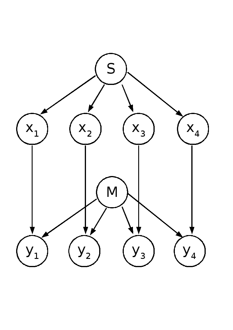
If and have been designed independently, their optimal joint description should be given by separate descriptions of and . However, the only feature of that is relevant for our observations is given by the distribution of -values, i.e., . Similarly, is the only relevant feature of . These features are directly given by observing the and the -values after infinite sampling. We therefore consider the algorithmic dependencies between and . Since the objects of our descriptions will be probability distributions, we introduce the following concept:
Definition 4 (computable functions and distributions).
Let denote some subset of .
A function is computable if there is a program that computes up to a precision for every input , for which has a finite description. Then denotes the length of the
shortest program of this kind. A probability distribution on a
finite probability space is called computable if its density is a computable function.
In the following section we apply the concepts introduced above to the case of strictly positive continuous densities .
3 Algorithmic dependencies induced by additive noise models
We have already argued that an additive noise model from to makes the causal structure unlikely because and then satisfy the non-generic relation of eq. (2). We now express this fact in terms of algorithmic information theory:
Theorem 1 (algorithmic dependence induced by an additive noise model).
Let be a two-times differentiable computable strictly positive probability density over .
If
admits an additive noise model from
to with a computable differentiable function , then
where and are arbitrary computable - and -values, respectively and .
Proof: Eq. (2) expresses the second derivative in terms of and . Hence,
| (7) |
We have by definition
| (8) |
The density is already determined by and the first derivative for some because then follows from normalization. Therefore,
where is some arbitrary prior information. Using , the right hand term of ineq. (8) yields
where the second inequality is due to ineq. (7).
The interpretation of Theorem 1 raises two problems: First, we cannot determine the exact ‘‘true’’ probabilities33 3 It is, anyway, a philosophical problem to what extent they are well-defined. from the observations, and second, we do not expect these probabilities to be computable, and hence it required an infinite amount of information to describe and if we could. As already pointed out in [6], algorithmic dependencies among the empirical distributions and after finite sampling do not show algorithmic dependencies between and . For continuous variables, this is already obvious from the fact that the conditional distribution of , given , is only defined for the support of . If the true distribution is a density, the empirical distribution contains every -value only once and knowing the support of thus already implies knowing .
To circumvent this problem, we will in the following section consider additive noise models over a finite probability space. Within this setting, we derive statements on distributions that are close to additive noise models. Since the finite case has the advantage that empirical frequencies converge pointwise to the true probabilities, this result also implies statements for the corresponding empirical distribution.
4 Stronger statements in finite probability spaces
The following theorem is a modification of Theorem 1 for additive noise models over the finite field for some prime number .
Theorem 2 (Algorithmic information between and for the discrete model).
Let be a computable strictly positive distribution on for some prime number that admits an additive noise model, i.e.,
there is a function
such that
and are statistically independent.
Here, subtraction is understood with respect to .
Then, if is non-constant, we have
| (9) |
Proof: The idea is, again, to derive an equation that shows that is essentially determined by up to some small amount of additional information. We have
Defining , for some for which , we introduce
| (10) |
which yields the equation
| (11) |
We interpret eq. (11) as a discrete version of eq. (2) because it relates differences between the values at different points to the quantity , which is a property of the conditional alone. Eq. (11) implies for arbitrary
for all . Writing for the vector with coefficients and for the vector with coefficients for , we rewrite eq. (11) as
where denotes the cyclic shift in dimension . Using the fact that is invertible on the space of vectors with zero sum of coefficients, we thus obtain
| (12) |
where is given by normalization and is the vector with only ones as entries. This shows that , , and determine . Denoting we can summarize the above into . This implies
because
where the second equality is due to the definition of conditional algorithmic mutual information (6).
We want to derive a similar lower bound for the case where almost admits an additive noise model. To this end, we first define a precision dependent Kolmogorov complexity of a probability distribution:
Definition 5 (Precision dependent algorithmic information).
Let be a density on
finite probability space. Let be a computable probability density and be the length of the
shortest program on a universal Turing machine that computes from .
Then
where denotes the relative entropy distance. Similarly, we define the conditional complexity given some prior information .
If is an arbitrary approximation of a distribution in the sense that holds for all , then and thus the precision dependent algorithmic information can be bounded from above by the complexity of the approximation: . For computable , we obviously have
but for uncomputable , the complexity tends to infinity. The following lemma shows the empirical content of precision-dependent complexity:
Lemma 2 (precision-dependent complexity of empirical distributions).
Let be a positive definite distribution on a finite probability space and be the empirical
distribution after -fold sampling from .
Then
with probability one.
Proof: Let be a distribution for which and . due to with probability one and because of the continuity of relative entropy for positive definite distributions we also have for all sufficiently large . Hence .
To prove that , let be a sequence of distributions such that and . Hence, for sufficiently large which completes the proof.
The following lemma will later be used to derive a lower bound on in terms of :
Lemma 3 (mutual information and approximative descriptions).
Let be a computable distribution on a finite probability space, an arbitrary string and
computable. Let be a distribution that is -close to , i.e.,
| (13) |
If can be derived from and from in the sense that
| (14) |
for additional strings and , then
Proof: Using the definition of conditional mutual information (6) we get
because Eq. (14) implies . On the other hand and therefore
In the same way, eq. (14) implies . A data processing inequality (Corrolary II.8 in [4]) then implies
We conclude with due to ineq. (13).
We will moreover need the following Lemma:
Lemma 4 (bound on the differences of logarithms).
Given a vector , we define a probability distribution by
where is the partition function. Let be defined by in the same way. Then
Proof: Due to
we only have to show
To this end, we define
Using the mean value theorem we have for an appropriate value
The last expression is the expected value of with respect to the probability distribution corresponding to , which cannot be greater than .
We now have introduced the technical requirements to formulate a theorem for approximate additive noise models:
Theorem 3 (approximate additive noise model).
Let be as in Theorem 2, but only admitting
an approximative additive noise model in the sense that
| (15) |
where is a lower bound on . Here, subtraction is understood with respect to . Then, if is non-constant, we have
| (16) |
Proof: The idea is to define a distribution that is close to and admits an exact additive noise model: Define a joint distribution on and by the product
By variable transformation, defines a distribution that admits an additive noise model from to . Eq. (11) now holds for and with instead of , which is defined similar to eq. (10). Denote the corresponding vector by . In analogy to eq. (12) and the proof of Theorem 2, we now have
where is the appropriate normalization constant and the all-one vector. To show that allows an approximative description of we have to replace and with and , respectively. We define
and using Lemma 4 we obtain
| (17) | |||||
The modulus of the eigenvalues of on this subspace are all smaller than (for ) since they read
We thus have
where the last inequality used . Together with , ineq. (17) then yields
| (18) |
Now we derive an upper bound on the two summands of the rhs. using our assumption on the limited statistical mutual information between and . To this end, we observe that
| (19) |
where the first equality is due to the invariance of relative entropy under variable transformation and the second uses a well-known reformulation of mutual information [3]. Moreover, we have
where denotes the conditional distribution for one specific value of . Using the lower bound on we obtain
Due to the well-known relation between relative entropy and -distance for two distributions [3], we obtain
This implies
| (20) |
by applying the mean value theorem to the function . From the definition of and in eq. (10) we conclude
| (21) |
On the other hand, (19) implies
and hence
| (22) |
Using ineqs. (21) and (22), ineq. (18) yields for all
| (23) |
Let be given by discretizing all values up to an accuracy of . Then
On the other hand, let be given by discretizing all values up to an accuracy of . Then and thus
Due to (23), both discretizations coincide up to one bit for each value , say . To illustrate this, consider the binary strings and which can be arbitrarily close despite their truncation being different. We conclude that
Let be the distribution generated by through normalization
Due to the upper bound (23), Lemma 4 gives
The theorem now follows from Lemma 3 applied to
The complexity of in the bound (16) will typically exceed the terms with because we will need several bits for every bin to describe the corresponding probability (this will be discussed in Section 5 in more detail). Moreover, can be quite low, in particular if we choose for some . Therefore, the mutual information between and is almost as large as the complexity of . This shows that the amount of adjustments required to mimic an additive noise model in the wrong direction depends essentially on the complexity of . In the following section we consider the complexity in the case in which is typical with respect to some known parametric family of distributions.
5 Kolmogorov complexity of distributions from a parametric family
The problem with applying Theorems 2 and 3 to real data is that the term cannot be known due to the uncomputability of Kolmogorov complexity in general. Fortunately, we can prove statements about the increase of the complexity for decreasing for typical elements of a family of distributions. This is shown by the following lemma:
Lemma 5 (typical distributions in parametric families).
Let be a parametric family of distributions over some finite probability space and
run over a -dimensional manifold .
Moreover, let be computable in the following sense:
there exists a program that computes for any computable input .
If the
Fisher information matrix has
full rank for all , the complexity of a typical distribution
grows logarithmically with decreasing , i.e. for sufficiently small
Proof: Let denote the Fisher information matrix of the parametric family and be the parameter vectors of all computable distributions that can be described with complexity .
For every we have [3]
| (24) |
For sufficiently small , the set of all with is thus contained in the ellipsoid
The volume of such an ellipsoid with respect to the Lebesque measure is given by
This can be seen by transforming the ellipsoid into a sphere of radius via the linear map .
Now we check how the minimum number of disjoint ellipsoids must increase with to cover at least a constant fraction of the parameter space . Otherwise, if the total volume tends to zero it gets more and more unlikely that it contains a randomly chosen . We need to increase proportional to and must increase with due to . Hence we need asymptotically at least bits.
To see that this is also sufficient, we consider a cube that we divide into equally sized cubes of side length with middle points such that
for any point in the same cube. By (24), this ensures for all and sufficiently small that . If is an upper bound for all eigenvalues of all it is sufficient to guarantee
This can be achieved by choosing
Hence it is sufficient to choose the smallest that satisfies
and whose th root is integer. The grid and thus every vector can be computed from and and can be computed from by assumption. Hence,
We will now apply Lemma 5 to the family of all distributions for which is bounded from below by some . It is canonically parameterized by the first probabilities if there are possible -values. Then we obtain:
Corollary 1 (algorithmic mutual information for typical distributions).
Proof: One can check that the Fisher information matrix has full rank. Then the proof of the preceding lemma shows for sufficiently small
Plugging this into the lower bound of Theorem 3 together with concludes the proof.
Hence, for typical , the lower bound is positive if and are large enough. This asymptotic statement still holds true if looks on a coarse-grained scale like some simple distribution , i.e., a Gaussian, but shows irregular deviations from if the probabilities are described more accurately.
To give an impression on the amount of information between and that can be inferred after -fold sampling, we recall that the mutual information between and can be estimated up to an accuracy of [12]. The lowest upper bound on in ineq. (15) that can be guaranteed by the observations thus is proportional to . Hence, for constant , the best lower bound on the amount of algorithmic information shared by and increases logarithmically in as long as the sample is not sufficient to reject independence between and .
6 Applying the results to empiricial distributions
In applying Theorems 2 and 3 to realistic situations, we still have the problem that we have no reason to believe that the true distribution is computable. On the other hand, applying the argument to the empirical distribution (which is, for large sampling close to an additive noise model) is still problematic because algorithmic dependencies between the empirical distribution and the empirical conditional do not prove algorithmic dependencies between the true distributions and . One reason is that every conditional probability can always be written as a fraction with denominator , which already is an algorithmic dependence.
We now describe how to use Postulate 1 if only a finite list of -pairs is observed and the underlying distribution is not known. Given samples , we can generate a non-empty subsample with high probability such that every -value occurs exactly -times. The samples can then be used for the estimation of . Hereby, is chosen independently of the samples in a way that for we have and the probability of obtaining from converges to one.
Now by construction, if contains no information about , the empirical distribution
of the subsample must not contain any information about the empirical distribution
of -values in the entire sample, i.e.,
| (25) |
In the spirit of [9], we postulate that the violation of eq. (25) indicates that the causal hypothesis is wrong or the mechanisms generating -values and the mechanisms generating -values from -values have not been generated independently. For a discussion of this case see [10]. Using this terminology, our goal is to derive a lower bound on for the case where admits an additive noise model from to . We can apply Theorem 3 to a distribution that is defined by the empirical results via
which is necessarily computable because it only contains rationale values.
We have already argued that the causal hypothesis would only be acceptable if
If the true distribution almost admits an additive noise model from to in the sense of ineq. (15), the same inequality will also be satisfied by if is sufficiently high and thus
provided that , which coincides with due to Lemma 2 for large , is high.
7 Approximating continuous variables with discrete ones
Causal inference via additive noise models has been described and tested for continuous variables [5]. We have discussed the discrete case mainly for technical reasons because we were able to prove statements for distributions that are only close to additive noise models. Our results can easily be applied to the continuous case by discretization with increasing number of bins. As already mentioned, the discretized version of the empirical distribution becomes computable, which circumvents the problem that the true distribution may be uncomputable.
Before we discuss the discretization in detail, we emphasize that there is a problem with applying Postulate 1 to the conditionals obtained after discretizing the variables: if we define a discrete variables and by putting and into bins each, the discretized conditional does not only depend on . Instead, it also contains information about the distribution of . For this reason, algorithmic dependencies between and only disprove the causal hypothesis if the binning is fine enough to guarantee that the discrete value is sufficient to determine the conditional probability for , i.e., the relevance of the exact value is negligible if the discrete value is given. It is therefore essential that the argument below refers to the asymptotic case of infinitely small binning.
To approximate a continuous density on by with increasing we consider the square
for all odd and replace with . We discretize into bins of equal size, which defines a probability distribution over -valued variables and , respectively. We define the function by putting the values with to the corresponding bin.
Moreover, appropriate smoothness asumptions on can guarantee that the mutual information between and converges to for . It is known [12] that there are estimators for mutual information that converge if the binning is increased proportionally to for sample size . If admits an additive noise model, i.e., , then . Hence, the discrete distributions on and get arbitrarily close to discrete additive noise models. Applying Theorem 2 to these discrete distributions then yields algorithmic dependence between the discretized marginal and the discretized conditional.
8 Conclusions
We have discussed a causal inference method that prefers the causal hypothesis to whenever the joint distribution admits an additive noise model from to and not vice versa. It seems that this way of reasoning assumes that all causal mechanisms in nature can be described by additive noise models (which is certainly not the case). Here we argue that the method is nevertheless justified because it is unlikely that a causal mechanism that is not of the form of an additive noise model generates a distribution that looks like an additive noise model in the wrong direction. This is because such a coincidence would require mutual adjustments between and . To measure the amount of tuning needed for this situation we have derived a lower bound on the algorithmic information shared by and . If we assume that “nature chooses” and independently, a significant amount of algorithmic information is not acceptable. Our justification of additive-noise-model based causal discovery thus is an application of two recent proposals for using algorithmic information theory in causal inference: [9] postulated that the shortest description of is given by separate descriptions of and , which would be violated then. [6] argued that algorithmic dependencies between any two objects require a causal explanation. They consider the two mechanisms that determine and , respectively, as two objects and conclude that the absence of causal links on the level of the two mechanisms imply their algorithmic independence, in agreement with [9].
References
- [1] G. Chaitin. On the length of programs for computing finite binary sequences. J. Assoc. Comput. Mach., 13:547–569, 1966.
- [2] G. Chaitin. A theory of program size formally identical to information theory. J. Assoc. Comput. Mach., 22:329–340, 1975.
- [3] T. Cover and J. Thomas. Elements of Information Theory. Wileys Series in Telecommunications, New York, 1991.
- [4] P. Gacs, J. Tromp, and P. Vitányi. Algorithmic statistics. IEEE Trans. Inf. Theory, 47(6):2443–2463, 2001.
- [5] P. Hoyer, D. Janzing, J. Mooij, J. Peters, and B Schölkopf. Nonlinear causal discovery with additive noise models. In D. Koller, D. Schuurmans, Y. Bengio, and L. Bottou, editors, Proceedings of the conference Neural Information Processing Systems (NIPS) 2008, Vancouver, Canada, 2009. MIT Press. http://books.nips.cc/papers/files/nips21/NIPS2008_0266.pdf.
- [6] D. Janzing and B. Schölkopf. Causal inference using the algorithmic Markov condition. http://arxiv.org/abs/0804.3678, 2008.
- [7] A. Kolmogorov. Three approaches to the quantitative definition of information. Problems Inform. Transmission, 1(1):1–7, 1965.
- [8] S. Lauritzen. Graphical Models. Clarendon Press, Oxford, New York, Oxford Statistical Science Series edition, 1996.
- [9] J. Lemeire and E. Dirkx. Causal models as minimal descriptions of multivariate systems. http://parallel.vub.ac.be/jan/, 2007.
- [10] J. Lemeire and K. Steenhaut. Inference of graphical causal models: Representing the meaningful information of probability distribution. To appear in Proceedings of the NIPS 2008 workshop “Causality - Objectives and Assessment”, edited by I. Guyon, D. Janzing, B. Schölkopf., 2009.
- [11] M. Li and P. Vitányi. An Introduction to Kolmogorov Complexity and its Applications. Springer, New York, 1997.
- [12] L. Paninski. Estimation of entropy and mutual information. Neural Computation, 15:1191–1254, 2003.
- [13] J. Pearl. Causality. Cambridge University Press, 2000.
- [14] H. Reichenbach. The direction of time. Dover, 1999.
- [15] R. Solomonoff. A preliminary report on a general theory of inductive inference. Technical report V-131, Report ZTB-138 Zator Co., 1960.
- [16] P. Spirtes, C. Glymour, and R. Scheines. Causation, prediction, and search (Lecture notes in statistics). Springer-Verlag, New York, NY, 1993.
- [17] K. Zhang and A. Hyvärinen. On the identifiability of the post-nonlinear causal model. In Proceedings of the 25th Conference on Uncertainty in Artificial Intelligence, Montreal, Canada, 2009.