Distribution functions for the Milky Way

We now consider the form of the function $f_{z}$ in equation (6), which controls the disc’s vertical structure. We focus on motion in the solar cylinder of stars for which $L_{z}\simeq R_{0}v_{\rm c}(R_{0})$ so they do not make large radial excursions. For these stars $f_{z}$ is effectively a function of only $J_{z}$. The classical choice of df is that of an isothermal sheet $f_{z}\sim{\rm e}^{-E_{z}/\sigma_{z}^{2}}$ (Spitzer, 1942). Our modelling strategy requires that we eliminate $E_{z}$ in favour of $J_{z}$. In a separable potential $\Omega_{z}J_{z}=\left\langle v_{z}^{2}\right\rangle$, where $\Omega_{z}=\partial E_{z}/\partial J_{z}$ is the vertical frequency and the angle brackets denote a time average along the orbit with action $J_{z}$. Moreover, by the virial theorem $\left\langle v_{z}^{2}\right\rangle=E_{z}$ in a harmonic oscillator, so we replace $E_{z}$ with $\Omega_{z}J_{z}$ and arrive at what we shall refer to as the “pseudo-isothermal” df

where the denominator ensures that $f_{\sigma_{z}}$ satisfies the normalisation condition

In general $\sigma_{z}$ is a function of $L_{z}$ to control the scale height as a function of radius, but for the moment we neglect this dependence and investigate the vertical density profile predicted by the df (7) by taking $\Phi_{z}(z)$ to be the potential above the Sun in Model II of §2.7 in BT08; this model is disc dominated.

The full curve in Fig. 1 shows the density profile predicted by the df (7) for $\sigma_{z}=6.3\,{\rm km}\,{\rm s}^{-1}$, while the dotted curve shows the classical isothermal $\rho\propto\exp(-\Phi/\sigma_{z}^{2})$. The two curves are very similar because equation (7) predicts that $\left\langle v_{z}^{2}\right\rangle^{1/2}$ moves in a narrow range from $6.55\,{\rm km}\,{\rm s}^{-1}$ at $z=0$ to a peak value $6.7\,{\rm km}\,{\rm s}^{-1}$ at $z=240\,{\rm pc}$. Both predictions are in reasonable agreement with the densities of A and F stars measured by Holmberg & Flynn (2000) shown by triangles and squares, respectively.

The dotted curve in the upper panel of Fig. 2 shows the vertical density profile predicted by equation (7) when $\sigma_{z}=18\,{\rm km}\,{\rm s}^{-1}$. The curvature of the profile has the wrong sign to fit the density profile of dwarfs with $4<M_{V}<5$ measured by Gilmore & Reid (1983), which is shown by circles. The velocity dispersion in this model is $\langle v_{z}\rangle^{1/2}=19.2\pm 0.3\,{\rm km}\,{\rm s}^{-1}$ independent of $z$, so the df is very close to an isothermal. The dotted curve in the lower panel shows that the Gaussian distribution in $v_{z}$ at $z=0$ predicted by the df is a poor fit to the distribution in $v_{z}$ of the GCS stars.

One way to obtain a vertical profile that is steeper at small heights and flatter at large heights is to replace the exponential in equation (7) with an algebraic function of $J_{z}$. The full curves in Fig. 2 show the density profile and velocity distribution predicted by the df

with $\gamma=2.6$ and $V_{\gamma}=18.7\,{\rm km}\,{\rm s}^{-1}$. The agreement with the data of Gilmore & Reid (1983) is essentially perfect. This fit, and all subsequent fits, were obtained by adjusting the parameters by hand and judging the quality of the fit by eye.

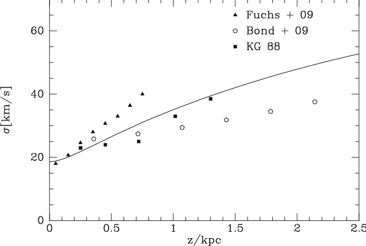
The curve in Fig. 3 shows the extent of the increase in velocity dispersion with height that is required to produce a thick-disc like flattening in the density profile at $z>500\,{\rm pc}$: $\left\langle v_{z}^{2}\right\rangle^{1/2}$ rises from $19.6\,{\rm km}\,{\rm s}^{-1}$ at $z=0$ to $37.5\,{\rm km}\,{\rm s}^{-1}$ at $z=1\,{\rm kpc}$ and $50.4\,{\rm km}\,{\rm s}^{-1}$ at $z=2\,{\rm kpc}$. Also shown are three sets of data points: filled squares show the values of $\sigma_{z}$ inferred by Kuijken & Gilmore (1989) (hereafter KG89) for the velocity dispersion of K dwarfs; filled triangles show the dispersion of metal-poor M dwarfs inferred by Fuchs et al. (2009); open pentagons show the analytic fit to the dispersions of disc stars that was published by Bond et al. (2009). Sadly, the data do not tell a coherent story. Each data set is for a different stellar population, so in principle their different trends in $\sigma_{z}(z)$ could be matched by different density profiles. Therefore in Fig. 2 we plot the density profiles associated with the Bond et al.  sample (Juric et al., 2008, from) and the KG89 sample. We see that the Juric et al. density profile is less steep than the one from KG89, which is inconsistent with the higher velocity dispersions measured by KG89. Fuchs et al. (2009) do not give a density profile, but it would be surprising if the kinematics and vertical structure of the M dwarfs were fundamentally different from that of the K dwarfs studied by KG89, so the extremely rapid increase in their values of $\sigma_{z}(z)$ shown in Fig. 3 is hard to understand.

The fact that the model curve in Fig. 3 agrees best with the KG89 may reflect the fact that the potential in which the df is evaluated was constrained to be compatible with value for the surface density of material that lies within $1.1\,{\rm kpc}$ of the plane given by Kuijken & Gilmore (1991), which was based on the KG89 data. In a gravitational potential tailored for the data of Juric et al. (2008) and Bond et al. (2009) the df might reproduce the data in these papers better than that of KG89. We do not pursue this question here.

Despite the simplicity of the df (9) and the accuracy with which it fits the data, we will not employ it further because it does not provide a decomposition of the disc into populations of different ages, and there is no natural way of incorporating it into a df that also describes the radial structure of the disc.

Star formation is known to have continued in the disc throughout the life of the Galaxy and the velocity dispersion of any cohort of coeval stars is known to increase secularly as a result of scattering by spiral arms and molecular clouds (Spitzer & Schwarzschild, 1953; Carlberg & Sellwood, 1985). Moreover, as the Galaxy ages, the chemical composition of the stars that are forming at a given radius changes, so stars formed at different times and different radii are in principle distinguishable. Hence it is useful to consider the disc’s aggregate df to be a sum of the dfs for stars of different ages and velocity dispersions.

We assume that the df of stars of age $\tau$ is the “pseudo-isothermal” df (7) with $\sigma_{z}$ increasing with $\tau$ according to (Aumer & Binney, 2009, e.g.)

Here $\sigma_{z0}$ is the velocity dispersion of stars at age $\tau_{\rm m}\simeq 10\,{\rm Gyr}$, $\tau_{1}$ sets velocity dispersion at birth, and $\beta\simeq 0.38$ is an index that determines how $\sigma_{z}$ grows with age. If we further assume that the rate of star formation has declined with time as ${\rm e}^{-t/t_{0}}$, then the aggregate df will be

where $\sigma_{z}$ depends on $\tau$ through equation (10). In Fig. 4 we plot the vertical density profile produced by this aggregate df when $t_{0}=8\,{\rm Gyr}$, $\tau_{1}=0.1\,{\rm Gyr}$, $\sigma_{z0}=20\,{\rm km}\,{\rm s}^{-1}$ (Aumer & Binney, 2009). We see that with these parameters we obtain a reasonable fit to the thin disc. Specifically, at $z{\,\mathrel{\mathchoice{\lower 2.9pt\vbox{\halign{$\m@th\displaystyle\hfil#\hfil$\cr>\crcr\sim\crcr}}}{\lower 2.9pt\vbox{\halign{$\m@th\textstyle\hfil#\hfil$\cr>\crcr\sim\crcr}}}{\lower 2.9pt\vbox{\halign{$\m@th\scriptstyle\hfil#\hfil$\cr>\crcr\sim\crcr}}}{\lower 2.9pt\vbox{\halign{$\m@th\scriptscriptstyle\hfil#\hfil$\cr>\crcr\sim\crcr}}}\,}}150\,{\rm pc}$ the density is nearly exponential with a scale height of $255\,{\rm pc}$. In view of the dramatic difference between this pure thin-disc structure and the thin plus thick disc structure furnished by the algebraic df (9), it is perhaps surprising that the velocity distribution in the lower panel of Fig. 4 differs as little as it does from the dashed curve in the lower panel of Fig. 2. This comparison illustrates an important point: thick-disc stars spend relatively little time near $z=0$ so they contribute only inconspicuous wings to the velocity distribution there. The velocity distribution predicted by $f_{\rm thn}$ is close to Gaussian: the velocity dispersion rises from $16.5\,{\rm km}\,{\rm s}^{-1}$ at $z=0$ to $19.6\,{\rm km}\,{\rm s}^{-1}$ at $z=500\,{\rm pc}$ and $20.9\,{\rm km}\,{\rm s}^{-1}$ at $z=1\,{\rm kpc}$.

Fig. 5 shows that a perfect fit to the Gilmore & Reid (1983) measurements can be obtained by adding a pseudo-isothermal component with $\sigma_{z}=38\,{\rm km}\,{\rm s}^{-1}$ to the thin disc shown in Fig. 4. Within this structure $\left\langle v_{z}^{2}\right\rangle^{1/2}$ increases from $19\,{\rm km}\,{\rm s}^{-1}$ at $z=0$ to $39\,{\rm km}\,{\rm s}^{-1}$ at $z=1.5\,{\rm kpc}$ and then very slowly increases to $41.5\,{\rm km}\,{\rm s}^{-1}$ at $z=2.5\,{\rm kpc}$. It is worth noting that adding the thick disc increases the scale height in the exponential fit to the profile at low $z$ from $255\,{\rm pc}$ to $336\,{\rm pc}$.

Shu (1969) discussed dfs for planar discs of the form

where $E_{\rm c}(L_{z})$ is the energy of a circular orbit of angular momentum $L_{z}$ and $\sigma_{r}(L_{z})$ is a function that determines the velocity dispersion in the disc as a function of radius. By analogy with the vertical df we could replace $E-E_{\rm c}$ by $\Omega_{r}J_{r}$, where $\Omega_{r}=\partial E/\partial J_{r}$ (Binney, 1987; Dehnen, 1999). However, the decrease in $\Omega_{r}$ as $J_{r}\to\infty$ is so rapid that for sufficiently eccentric orbits the product $\Omega_{r}J_{r}$ decreases with increasing $J_{r}$. Consequently, if one substitutes $\Omega_{r}J_{r}$ for $E-E_{\rm c}$, at fixed $L_{z}$ and large $J_{r}$ the df increases with $J_{r}$. To prevent this unphysical behaviour we replace $E-E_{\rm c}$ by $\kappa J_{r}$, where

is the epicycle frequency. Hence in this paper we adopt as the planar df of a pseudo-isothermal population

In view of the normalisation condition (8), the mass ${\rm d}M$ placed by the df (6) on orbits with angular momentum in the range $(L_{z},L_{z}+{\rm d}L_{z})$ is

In the limit $\sigma_{r}\to 0$ of a cold disc, only circular orbits are populated and this mass is equal to the mass $2\pi\Sigma R\,{\rm d}R$ in the annulus $(R,R+{\rm d}R)$, where $\Sigma$ is the disc’s surface density. Hence for a cold disc

where $R_{\rm c}(L_{z})$ is the radius of the circular orbit of angular momentum $L_{z}$ and the second equality uses the identity ${\rm d}L_{z}/{\rm d}R=R\kappa^{2}/2\Omega$. Here we consider the case of an exponential disc, $\Sigma=\Sigma_{0}{\rm e}^{-(R-R_{0})/R_{\rm d}}$, where $R_{\rm d}\simeq 2.5\,{\rm kpc}$ is the scale length of the disc and $R_{0}\simeq 8\,{\rm kpc}$ is the Sun’s distance from the Galactic centre. We assume that $\sigma_{r}$ declines exponentially in radius with a scale length that is roughly twice that of the surface density

This choice is motivated by naive epicycle theory, which implies that with $q\simeq 0.5$ the scale height will be constant (van der Kruit & Searle, 1982) provided $\sigma_{z}/\sigma_{r}=\hbox{constant}$.

A df such as $f_{1}$ times equation (14) that is an even function of $L_{z}$ does not endow the Galaxy with rotation. We introduce rotation by adding to the df an odd function of $L_{z}$, which will not contribute to either the surface density or the radial velocity dispersion. A convenient choice for this odd contribution to the df is $\tanh(L_{z}/L_{0})$ times the even contribution, where $L_{0}$ is a constant that determines the steepness of the rotation curve in the central region of solid-body rotation. At radii so large that $Rv_{\rm c}\gg L_{0}$ this choice for the odd part of the df simply eliminates counter-rotating stars. We choose $L_{0}=10\,{\rm km}\,{\rm s}^{-1}\,{\rm kpc}$, a value sufficiently small for counter-rotating stars to be confined to the inner kiloparsec of the Galaxy, which is in reality bulge-dominated. Hence we consider the “pseudo-isothermal” planar df

It is interesting to evaluate the observables predicted by the df (18) when the circular speed is a power law in $R$, $v_{c}=v_{0}(R/R_{0})^{\alpha/2}$. Then

In the limit $\alpha\to 0$ of a perfectly flat circular speed

Fig. 6 shows the surface density, rotation curve and radial velocity-dispersion profile predicted by the pseudo-isothermal df (18) for a flat circular-speed curve with $v_{0}=220\,{\rm km}\,{\rm s}^{-1}$. For the plotted profiles the function $\Sigma(R_{\rm c})$ has been taken to be an exponential of scale length $2.25\,{\rm kpc}$, while the full curve in the top panel shows that the surface density produced by this choice of $\Sigma(R_{\rm c})$ provides a good approximation to the surface density of an exponential disc with a longer scale length, $2.5\,{\rm kpc}$, which is shown by the dashed line. At the price of replacing the analytic function

with a tabulated function, the surface density can be made exactly exponential (Dehnen, 1999). Here we adopt the simpler expedient of using a slightly smaller value of $R_{\rm d}$ than the scale length of the disc we wish to produce.

In the middle panel of Fig. 6 the mean rotation speed declines from $225\,{\rm km}\,{\rm s}^{-1}$ at $R=1\,{\rm kpc}$ to $\sim 200\,{\rm km}\,{\rm s}^{-1}$ at $R=5\,{\rm kpc}$ before slowly rising to $210\,{\rm km}\,{\rm s}^{-1}$ at $R=10\,{\rm kpc}$. The bottom panel shows that the radial velocity dispersion declines throughout the disc as expected, being $\sim 34\,{\rm km}\,{\rm s}^{-1}$ at $R_{0}$.

Fig. 7 compares the distributions of $v_{\phi}$ and $v_{R}$ velocities predicted by the pseudo-isothermal df with the corresponding distributions of GCS stars with heliocentric velocities converted to $v_{\phi}$ and $v_{R}$ assuming that the circular speed is $220\,{\rm km}\,{\rm s}^{-1}$ and the Sun’s velocity is $v_{R}=-10\,{\rm km}\,{\rm s}^{-1}$, $v_{\phi}=v_{\rm c}+5.2\,{\rm km}\,{\rm s}^{-1}$ (Dehnen & Binney, 1998, hereafter DB98). The theoretical and observed distributions in $v_{R}$ are satisfyingly similar, but the theoretical $v_{\phi}$ distribution lies above the observed distribution at small $v_{\phi}$ and well below it at $v_{\phi}\sim 200\,{\rm km}\,{\rm s}^{-1}$. We return to this issue below.

As discussed in Section 2.1, realistically we must consider the thin disc to be a superposition of pseudo-isothermal cohorts of different ages and chemical compositions. The temperature of the pseudo-isothermal df (18) is set by the parameter $\sigma_{r0}$ through equation (17). By analogy with equation (10), we should make $\sigma_{r}$ age dependent by adding to the right side of this equation the appropriate function of $\tau$. Then $\sigma_{r}$ is given by

With $\sigma_{r}(L_{z},\tau)$ thus defined, it is natural to consider the thin-disc df

where $f_{\sigma_{r}}$ is defined by equation (18) with $\sigma_{r}(L_{z},\tau)$ now obtained from equation (22). The df $\overline{f}(J_{r},L_{z})$ correctly yields values of observables averaged through the thickness of the disc. In the case of an external galaxy such averaged observables are of interest, but samples of Milky-Way stars rarely if ever provide a sample that is unbiased in $z$. In particular, stars with large $J_{z}$ spend little time near the Sun so samples of local stars are biased against them. Since a star with large $J_{z}$ is likely to be old, it is likely to have large $J_{r}$ also. Hence samples of local stars are biased towards small $J_{r}$ and the df (23) cannot be used to predict the properties of solar-neighbourhood stars, or indeed stars at that lie within any restricted range in $z$. Instead we must use the full thin-disc df.

At the end of Section 2.1 we saw that the observed vertical density profile at the Sun can be reproduced by adding to the composite df of the thin disc a pseudo-isothermal component with $\sigma_{z0}=38\,{\rm km}\,{\rm s}^{-1}$ that contains 20 percent of the mass. This result suggests that we add to the df (24) of the thin disc the thick-disc df

where $f_{\sigma_{r}}$ and $f_{\sigma_{z}}$ are defined by equations (18) and (7) above with $\sigma_{r}$ and $\sigma_{z}$ given by

and in equation (18) we use (cf eq. 21)

Here $k_{\rm thk}$ is the ratio of thick to thin-disc stars in the solar cylinder. In principle this thick-disc df introduces a further six parameters: $L_{0}$, $R_{\rm d}$, $q$, $\sigma_{r0}$, $\sigma_{z0}$ and $k_{\rm thk}$. Table 1 lists all the parameters of the standard df. We have not explored the option of using a different value of $L_{0}$ for each disc because this parameter has a negligible impact on comparisons with local data.

The choice of $\sigma_{z0}$ and $k_{\rm thk}$ for the thick disc is straightforwardly made by the requirement that the vertical density profile match the data of Gilmore & Reid (1983). The choice of $R_{\rm d}$, $q$ and $\sigma_{r0}$ for the thick disc is more problematic. Clearly these parameters should be constrained by the radial density and kinematics of the disc at $z>1\,{\rm kpc}$, where the thick disc is dominant. The strongest constraints are provided by the SDSS. Juric et al. (2008) found the scalelength of the thick disc to be similar to that of the thin disc. Bond et al. (2009) give an analytic fit to the dependence of $\sigma_{R}$ on $z$ out to $z\simeq 4\,{\rm kpc}$, and Fuchs et al. (2009) give several values of $\sigma_{R}$ at $z\leq 800\,{\rm pc}$. Finally Ivezic et al. (2008) provide distributions in $v_{\phi}$ in several ranges of $z$. Figs 8 and 9 show these data.

Although the data sets are less clearly inconsistent than they are in Fig. 3, the data from Fuchs et al. clearly show a significantly steeper gradient than those from Bond et al. In the model $\sigma_{R}(z)$ has a slope intermediate between these values, and agrees with the data at $z{\,\mathrel{\mathchoice{\lower 2.9pt\vbox{\halign{$\m@th\displaystyle\hfil#\hfil$\cr<\crcr\sim\crcr}}}{\lower 2.9pt\vbox{\halign{$\m@th\textstyle\hfil#\hfil$\cr<\crcr\sim\crcr}}}{\lower 2.9pt\vbox{\halign{$\m@th\scriptstyle\hfil#\hfil$\cr<\crcr\sim\crcr}}}{\lower 2.9pt\vbox{\halign{$\m@th\scriptscriptstyle\hfil#\hfil$\cr<\crcr\sim\crcr}}}\,}}1\,{\rm kpc}$. At greater heights it lies above the Bond et al. data, just as the model curve does in Fig. 3.

The model’s predictions for the distribution in $v_{\phi}$ at $z=1\,{\rm kpc}$ and $z=1.75\,{\rm kpc}$ are shown in Fig. 9 together with data points from Ivezic et al. (2008) the heliocentric data of Ivezic et al. (2008) have been converted to galactocentric velocities assuming $v_{\phi}(\odot)=225.2\,{\rm km}\,{\rm s}^{-1}$, which arises because in our adopted potential the circular speed is $220\,{\rm km}\,{\rm s}^{-1}$ and the peculiar $V$ velocity of the Sun is $5.2\,{\rm km}\,{\rm s}^{-1}$ (Dehnen & Binney, 1998). The full curves are the true model velocity distributions, and the dotted curves show the result of convolving these distributions with the errors reported by Ivezic et al., which are $19.5\,{\rm km}\,{\rm s}^{-1}$ at $z=1\,{\rm kpc}$ and $31.5\,{\rm km}\,{\rm s}^{-1}$ at $z=1.75\,{\rm kpc}$.

The model curves fall below the data at $v_{\phi}\la 50\,{\rm km}\,{\rm s}^{-1}$ because in this region halo stars dominate the data points and the model is for the disc alone. Elsewhere the dotted curves provide a moderate fit to the data points. The fit in the upper panel would be improved by moving the data points a few $\!\,{\rm km}\,{\rm s}^{-1}$ to the right, which would be the effect of the upward revision of the Sun’s peculiar velocity advocated below. The model curves are slightly too broad. Reducing the parameter $\sigma_{r}$ in the thick-disc df makes them narrower, but this change also shifts the model curves still further to the right, and thus makes the overall fit less good. The distributions can also be made narrower by either increasing the thick-disc scalelength $R_{\rm d}$ or by decreasing $q$. However either change decreases the importance of stars at apocentre (which have angular momentum $L_{z}<L_{z}(\odot)$) relative to those at pericentre and thus exacerbates the predicted excess of stars at large $v_{\phi}$. Extensive experimentation suggests that the fits shown in Fig. 9 cannot be significantly improved upon with a df of the form (26).

Because they are extracted from proper-motion data, the observational distributions in Fig. 9 are sensitive to the photometric distances employed. A possible resolution of the conflict in the lower panel of Fig. 9 between the model and data is that the distances employed are slightly too small: using larger distances would increase heliocentric velocities and thus cause the observational points to move away from the Sun’s assumed velocity, $v_{\phi}=225.2\,{\rm km}\,{\rm s}^{-1}$. Another possible resolution of the conflict between data and models in Fig. 9 is the increasing inaccuracy of the assumption of adiabatic invariance of the vertical motion as random motions become more important. In a future publication this possibility will be examined with models based on orbital tori.

Fig. 10 shows prediction of the standard df for the structure of the solar neighbourhood. Full curves are for the whole disc and dashed curves show the contribution of the thin disc. The upper panels show for stars seen in the plane the distributions in $v_{\phi}$ and $v_{R}$ after integrating over the other two velocity components. Comparison of these panels with the panels of Fig. 7 is instructive. The distribution of $v_{R}$ velocities is in reasonable agreement with the data, while the distribution of $v_{\phi}$ velocities of Fig. 10 agrees with the data better than the distribution in $v_{\phi}$ in Fig. 7. Two factors contribute to the improved fit to the $v_{\phi}$ velocities. First introducing a sum of pseudo-isothermals enhances both the core and the wings of the distribution – this effect is apparent in the distributions of $v_{R}$ velocities. More significantly, including vertical motion suppresses the $v_{\phi}$ distribution at low $v_{\phi}$ because this wing of the distribution is populated by stars with small values of $R_{\rm c}$ that reach the solar neighbourhood because they have large random velocities. On account of those large velocities, they have low probabilities of being found close enough to the plane to be included in the GCS. These stars are most likely to be observed near apocentre, when they have low values of $v_{R}$, so depressing the contribution to the GCS of such stars does not suppress the wings of the distribution of $v_{R}$ velocities.

The plots shown in Fig. 10 are obtained by setting the function $\Sigma(R_{\rm c})$ for the thin disc that appears in the df to the same exponential with scale length $2.25\,{\rm kpc}$ that was used to obtain Figs 6 and 7. The use of $2.25\,{\rm kpc}$ in $\Sigma(R_{\rm c})$ is important not only to ensure that the disc’s surface density is approximately exponential with the larger scale length $2.5\,{\rm kpc}$, but also to ensure that the predicted distribution of $v_{\phi}$ velocities agrees with the GCS data: when $\Sigma$ has scale length $2.5\,{\rm kpc}$, the predicted distribution falls off too slowly at $v_{\phi}>v_{\rm c}$.

The model $v_{\phi}$ distribution deviates from the data in two respects: it lacks the pronounced peak in the data centred on $v_{\phi}=205\,{\rm km}\,{\rm s}^{-1}$, and it extends too far on the high-velocity wing. The first shortcoming undoubtedly reflects the axisymmetry of the model and is discussed below. The second shortcoming, which is also evident in the fits to the data of Ivezic et al. (2008) for the thick disc (Fig. 9), is more interesting. It can be moderated by increasing the parameter $q$ of equation (22). This parameter controls the radial gradient of the thin disc’s velocity dispersion, and a rapid decrease in the amplitude of epicycle motions at $R_{\rm c}>R_{0}$ limits the number of stars with large angular momentum that can reach the Sun and thus depopulates the high-$v_{\phi}$ wing. However, an increase in $q$ boosts the model profile at low $v_{\phi}$, so the overall agreement with the data is not improved unless the parameter $\sigma_{r0}$ of equation (22) is simultaneously decreased, and such a decrease leads to the model $v_{R}$ distribution being narrower than the data warrant.

Oort’s relation e.g., BT08 eq. (4.317)

implies that the width of the model $v_{\phi}$ distribution can be decreased relative to that of the $v_{R}$ distribution by changing from a flat to a falling circular-speed curve. However, one finds that the relative narrowing of the $v_{\phi}$ distribution that is produced by adopting the power-law potential (19) with $\alpha=-0.2$ produces a negligible improvement on the fit for constant circular speed shown in Fig. 10.

The bottom left panel of Fig. 10 shows that the overall df provides an excellent fit to the vertical density profile from Gilmore & Reid (1983), and that the vertical profile of the thin disc is extremely close to exponential. The latter result appears to be fortuitous in that it involves a subtle interplay between the non-trivial vertical force law and the number of stars with large random velocities that visit the solar neighbourhood from significantly nearer the Galactic centre.

The bottom right panel of Fig. 10 shows that in both the thin and thick discs the mean rotation speed declines with distance from the plane. In the plane the thin disc rotates faster than the thick disc, as one naively expects. However, the rotation rate of the thin disc declines faster with $z$ than that of the thick disc. The slower decline in the thick disc arises because we have set $R_{\rm d}=2.3\,{\rm kpc}$ in the function $\Sigma(R_{\rm c})={\rm e}^{-R_{\rm c}/R_{\rm d}}$ for the thick disc – with $R_{\rm d}=2.25\,{\rm kpc}$ for both discs the thick disc rotates $\sim 15\,{\rm km}\,{\rm s}^{-1}$ slower than the thin disc at all values of $z$. We have chosen $R_{\rm d}=2.3\,{\rm kpc}$ for the thick disc to obtain a better fit to the long-dashed curve in the lower right panel of Fig. 10, which is an analytic fit to the mean rotation rate extracted from the proper motions of SDSS stars by Ivezic et al. (2008). The dependence of the rotation rate on $R_{\rm d}$ is consistent with the Stromberg equation

For our preferred df the asymmetric drift of the thick disc increases from only $20\,{\rm km}\,{\rm s}^{-1}$ at $z=0$ to $90\,{\rm km}\,{\rm s}^{-1}$ at $z=3\,{\rm kpc}$, consistent with the values $30-50\,{\rm km}\,{\rm s}^{-1}$ usually reported by observers (Edvardsson et al., 1993; Gilmore et al., 1989, e.g.).

Fig. 11 compares the observed density of stars in the plane of velocities $(U,V)$ with respect to the LSR¹¹ 1 We follow BT08 (p. 12) in defining the LSR to be $v_{R}=v_{z}=0$ and $v_{\phi}=v_{\rm c}(R_{0})$. The LSR is sometimes taken to be the speed of a closed orbit through $R_{0}$. In the presence of ephemeral spiral structure this second definition is probably not useful. (top panel) to that predicted by the standard df (bottom). The dynamic range in density that can be sampled with the GCS stars is limited, so only a portion of the standard df’s predictions for the $(U,V)$ plane is tested. Moreover, the limited number of GCS stars leads to the steepness of density gradients being underestimated, for example around $(U,V)=(0,40)\,{\rm km}\,{\rm s}^{-1}$.

Near $(U,V)=(0,0)$, the observational diagram shows density enhancements, or “streams”, that are not bounded by the roughly ellipsoidal surfaces in velocity space on which actions are constant. Consequently, by Jeans’ theorem, the presence of streams indicates that either the Galaxy’s potential is not axisymmetric, or the Galaxy is not in a steady state – no df that is a function of actions only can reproduce these streams, although one hopes to be able to reproduce them by perturbing such a df using Hamiltonian perturbation theory. The streams account for much of the disagreement between the theoretical and observed velocity distributions in Fig. 10. In particular they account for the peak in the observed $v_{\phi}$ distribution lying $\sim 15\,{\rm km}\,{\rm s}^{-1}$ below the circular speed.

We have seen that the df has difficulty simultaneously fitting the observed distributions in $v_{R}$ and $v_{\phi}$ of the GCS stars (top panels of Fig. 10). A related problem was encountered in the fit to the proper motions of thick-disc stars (Fig. 9). The agreement between theory and data in both figures would be improved by shifting the observed $v_{\phi}$ distribution to the right. Such a shift would correspond to increasing the Sun’s peculiar velocity by a few kilometers per second.

Although such a shift significantly exceeds the formal error of $0.6\,{\rm km}\,{\rm s}^{-1}$ on $V_{\odot}$ given by DB98, we should not lightly dismiss the possibility that $V_{\odot}$ has been underestimated. The value given by DB98 was obtained by extrapolating to zero velocity dispersion a plot of $V$ velocity versus squared velocity dispersion $S^{2}$ for stars grouped by colour such as that shown in Fig. 12. Stromberg’s equation (30) suggests that this relation will be linear if the square bracket is constant, and Fig. 12 shows that the Hipparcos data are consistent with this expectation if the groups with the lowest velocity dispersions (shown in red) are discounted. However, Stromberg’s equation is obtained under the assumption that the Galactic potential is axisymmetric, so in the limit of vanishing velocity dispersion, stars move on circular orbits. In reality the potential has a non-axisymmetric component of amplitude $\sim 7\,{\rm km}\,{\rm s}^{-1}$, which manifests itself, inter alia, by causing a plot of terminal velocity versus Galactic longitude to undulate at this level (e.g. Malhotra, 1995; Binney & Merrifield, 1998, Fig. 9.16). Given the non-axisymmetric component of the potential, $\lim_{\sigma\to 0}\left\langle V\right\rangle$ can differ from the velocity of circular motion by of order the amplitude $\sim 7\,{\rm km}\,{\rm s}^{-1}$ of the non-axisymmetric component.

As Olling & Dehnen (2003) pointed out in their determination of the Oort constants, the larger the velocity dispersion a population has, the less it is likely to be affected by non-axisymmetric forces associated with spiral structure. The non-axisymmetric potential of the Galaxy’s bar is thought to be responsible for the “Hercules stream”, an over-density of stars in velocity space around $v_{\phi}=v_{\rm c}-50\,{\rm km}\,{\rm s}^{-1}$, but there is no evidence that it significantly perturbs the velocity distribution at $v_{\phi}{\,\mathrel{\mathchoice{\lower 2.9pt\vbox{\halign{$\m@th\displaystyle\hfil#\hfil$\cr>\crcr\sim\crcr}}}{\lower 2.9pt\vbox{\halign{$\m@th\textstyle\hfil#\hfil$\cr>\crcr\sim\crcr}}}{\lower 2.9pt\vbox{\halign{$\m@th\scriptstyle\hfil#\hfil$\cr>\crcr\sim\crcr}}}{\lower 2.9pt\vbox{\halign{$\m@th\scriptscriptstyle\hfil#\hfil$\cr>\crcr\sim\crcr}}}\,}}v_{\rm c}$, where the standard model conflicts with the data. Consequently, Fig. 10 offers an opportunity to determine $V_{\odot}$ that is at least as valid as the traditional route using Stromberg’s equation.

The jagged curve in the upper panel of Fig. 13 shows the cumulative distribution in $v_{\phi}$ of the GCS stars under the assumption that $v_{\rm c}(R_{0})=220\,{\rm km}\,{\rm s}^{-1}$ and $V_{\odot}=5.2\,{\rm km}\,{\rm s}^{-1}$. The smooth curve shows the cumulative distribution of the model shown in Fig. 10. The need to shift the distribution of GCS stars to the right is evident.

The full curve in the lower panel of Fig. 13 shows the Kolmogorov–Smirnov probability $P_{\rm KS}$ that the distribution of $V$ velocities of GCS stars is drawn from the model shown in Fig. 10 as a function of the amount $\Delta V$ added to the solar motion given in DB98. For all choices of $\Delta V$, $P_{\rm KS}$ is small, largely due to the impact of streams on the data for $-20\,{\rm km}\,{\rm s}^{-1}{\,\mathrel{\mathchoice{\lower 2.9pt\vbox{\halign{$\m@th\displaystyle\hfil#\hfil$\cr<\crcr\sim\crcr}}}{\lower 2.9pt\vbox{\halign{$\m@th\textstyle\hfil#\hfil$\cr<\crcr\sim\crcr}}}{\lower 2.9pt\vbox{\halign{$\m@th\scriptstyle\hfil#\hfil$\cr<\crcr\sim\crcr}}}{\lower 2.9pt\vbox{\halign{$\m@th\scriptscriptstyle\hfil#\hfil$\cr<\crcr\sim\crcr}}}\,}}V_{\rm LSR}{\,\mathrel{\mathchoice{\lower 2.9pt\vbox{\halign{$\m@th\displaystyle\hfil#\hfil$\cr<\crcr\sim\crcr}}}{\lower 2.9pt\vbox{\halign{$\m@th\textstyle\hfil#\hfil$\cr<\crcr\sim\crcr}}}{\lower 2.9pt\vbox{\halign{$\m@th\scriptstyle\hfil#\hfil$\cr<\crcr\sim\crcr}}}{\lower 2.9pt\vbox{\halign{$\m@th\scriptscriptstyle\hfil#\hfil$\cr<\crcr\sim\crcr}}}\,}}10\,{\rm km}\,{\rm s}^{-1}$. The impact of streams on $P_{\rm KS}$ can be reduced by randomly redistributing stars within this range of $V_{\rm LSR}$. The dotted curve in Fig. 13 shows the dependence of $P_{\rm KS}$ on $\Delta V$ when the randomised sample is compared to the model. The peak in $P_{\rm KS}$ rises by three orders of magnitude and shifts from $\Delta V=6.9\,{\rm km}\,{\rm s}^{-1}$ to $5.8\,{\rm km}\,{\rm s}^{-1}$.

Thus the stars that should be least affected by spiral structure suggest that DB98 underestimated $V_{\odot}$ by $\Delta V=5.8\,{\rm km}\,{\rm s}^{-1}$, so the true solar motion is $V_{\odot}=11\,{\rm km}\,{\rm s}^{-1}$. The systematic error $\sim 1\,{\rm km}\,{\rm s}^{-1}$ on this value is clearly much greater than the formal error reported by DB98. In Fig. 12 the black rectangle marks this revised solar motion.

It is interesting to test the extent to which Stromberg’s equation is verified by pseudo-isothermal dfs for main-sequence stars of a given colour. The dashed curve in Fig. 12 shows the relation between $S^{2}\simeq(1.2\sigma_{R})^{2}$ (DB98) and $V_{\rm a}$ that one obtains by calculating these quantities for a df of the form (24) with $\tau_{\rm m}$ increasing from $1$ to $11\,{\rm Gyr}$; over this age range $\sigma_{R}$ increases from $12.4$ to $28\,{\rm km}\,{\rm s}^{-1}$. The dashed curve is plotted on the assumption that the solar motion is $V_{\odot}=11\,{\rm km}\,{\rm s}^{-1}$, as marked by the black rectangle. At low $S^{2}$ the slope of the dashed curve is similar to the slope of the observational relation, but the slope flattens perceptibly with increasing $S^{2}$. This flattening implies that the square bracket in Stromberg equation (30) diminishes with increasing velocity dispersion. The is no evident reason why this bracket should be constant.

It is not inconceivable that spiral structure and/or the bar have shifted the observational points with $S^{2}$ in the range $(250,700)$ downwards from a relation that runs from the black square, between the red points and on to just above the points at $S^{2}>1200$. Moreover, a proponent of the conventional value of $V_{\odot}$ should worry that if the dashed curve were moved down to start at that value of $V_{\odot}$, it would lie below nearly all the data points. We conclude that although we cannot confidently recommend an upward revision of $V_{\odot}$, considerable caution should be exercised in the use of the conventional value and more work is needed on the effect that spiral structure has on the local velocity space.

Analysis of the space velocities of 18 maser sources for which trigonometric parallaxes are available (Reid et al., 2009) provides tentative support for $V_{\odot}$ being revised upwards to $11\,{\rm km}\,{\rm s}^{-1}$ (McMillan & Binney, 2009).

The values of $V_{\odot}$, the proper motion of Sgr A^∗, $6.38\pm 0.04\,\hbox{mas\,s}^{-1}$ (Reid & Brunthaler, 2004), and the distance to Sgr, A^∗, $8.33\pm 0.31\,{\rm kpc}$ (Gillessen et al., 2009), determine the local circular speed $v_{\rm c}(R_{0})=R_{0}\mu_{A*}-V_{\odot}=(251\pm 12-V_{\odot})\,{\rm km}\,{\rm s}^{-1}$. Flynn et al. (2006) estimate the absolute I-band luminosity of the Galaxy to be $M_{I}=-22.3$. At this absolute magnitude the ridge-line of the I-band Tully–Fisher relation (Dale et al., 1999) gives a circular speed of only $190\,{\rm km}\,{\rm s}^{-1}$; $251\,{\rm km}\,{\rm s}^{-1}$ lies $2.6\sigma$ from the ridge line. Thus the likelihood of the Galaxy in the context of the Tully–Fisher relation is small but increases rapidly with $V_{\odot}$, and this fact provides further support for an upward revision of $V_{\odot}$.

Studies of the chemistry of the thick disc depend heavily on identifying nearby, bright stars that belong to the thick disc as targets of medium-dispersion spectroscopy (Fuhrmann, 1998; Bensby et al., 2003; Venn et al., 2004; Bensby et al., 2005; Gilli et al., 2006; Reddy et al., 2006). A popular strategy for identifying target stars is to assume ellipsoidal velocity distributions for each disc of the form (Bensby et al., 2003)

where $(U,V,W)$ are velocity components with respect to the LSR, and each component is assigned assumed values of $\sigma_{U},\sigma_{V},\sigma_{W}$ and the rotational lag $V_{\rm a}$. A given star is assigned to the population for which it gives the largest value of the df that follows from equation (31) and assumed fractions of local stars that belong to each population.

The idea behind equation (31) is that, for appropriate parameters, $f$ provides a useful approximation to the dfs of the two discs. Here we investigate the quality of this approximation by comparing $f$ with the thin- and thick-disc components of the standard df when the parameters in $f$ take the values used by Bensby et al. (2003), which are given in Table 1. Fig. 14 quantifies the quality of the approximation provided by $f$ by reporting the fractional rms variation in the appropriate component of the standard df over each ellipsoidal surface in velocity space on which $f$ is constant (dotted curves) – ideally this would vanish. The full curves show the mean value of the df over an ellipsoid of constant $f$, divided by the value of $f$ on that ellipsoid – since the normalisation of $f$ is arbitrary, the full lines in Fig. 14 may be shifted up or down at will, but must be horizontal if $f$ it to provide a useful approximation to the relevant component of the standard df.

The upper panel of Fig. 14 is for the thin disc and the lower panel for the thick disc. Since the full curve in the upper panel is approximately horizontal, we conclude that $f$ decreases from small to large ellipsoids in the same way that our model thin-disc df does. However, from the fact that the dotted curve lies above $0.7$ for $a>\sigma_{U}$, we conclude that the model df varies by of order itself over the larger velocity ellipsoids of the thin disc. Thus $f$ is a useful but not very accurate approximation to the model df for the thin disc.

The lower panel of Fig. 14 implies that $f$ provides a very poor approximation to our model thick-disc df: not only does the full curve rise by more than a factor of 4 as $a$ increases to $2\sigma_{U}$, but the essentially linear rise of the dotted curve implies that the model df varies strongly over ellipsoids of constant $f$. What prevents $f$ providing a good approximation to the df is the continuous increase in the asymmetric drift as the numerical value of the df decreases. This increase is apparent in the downward motion of isodensity contours in Fig. 11 and drives the fall in $\langle v_{\phi}\rangle$ with $z$ in the bottom right panel of Fig. 10. In particular, at $z=0$ the density of stars in velocity space peaks close to the circular speed in the thick disc as in the thin. This fact conflicts with the structure of equation (31).

The standard df predicts that the distribution of stars in the $(v_{R},v_{\phi})$ plane at height $z$ and $v_{z}=0$ is identical to the $(v_{R},v_{\phi})$ distribution of stars at any other height $z^{\prime}<z$ and velocity $v_{z}^{\prime}=\{2[\Phi_{z}(z)-\Phi_{z}(z^{\prime})]\}^{1/2}$. Moreover, a sample of stars observed at some distance $z$ from the plane will be heavily weighted towards stars whose vertical motions have turning points there. So there should be a close correspondence between local stars with a particular value of $v_{z}$ and samples of stars at a given value of $z$. Since the SDSS and its successors provide photometric distances and proper motions for millions of stars that lie ${\,\mathrel{\mathchoice{\lower 2.9pt\vbox{\halign{$\m@th\displaystyle\hfil#\hfil$\cr>\crcr\sim\crcr}}}{\lower 2.9pt\vbox{\halign{$\m@th\textstyle\hfil#\hfil$\cr>\crcr\sim\crcr}}}{\lower 2.9pt\vbox{\halign{$\m@th\scriptstyle\hfil#\hfil$\cr>\crcr\sim\crcr}}}{\lower 2.9pt\vbox{\halign{$\m@th\scriptscriptstyle\hfil#\hfil$\cr>\crcr\sim\crcr}}}\,}}1\,{\rm kpc}$ from the plane, and the GCS catalogue provides space velocities for over ten thousand nearby stars, this correspondence can be tested in some detail. Fig. 15 shows some sample $(v_{R},v_{\phi})$ distributions.

References

- Abazajian (2009) Abazajian K., et al., 2009, ApJS, 182, 543-558
- Ascasibar & Binney (2005) Ascasibar Y., Binney J., 2005, MNRAS, 356, 872
- Aumer & Binney (2009) Aumer M., Binney J., 2009, MNRAS, in press (arXiv 0905.2512)
- Bensby et al. (2003) Bensby T., Feltzing S., Lundström I., 2003, A&A, 410, 527
- Bensby et al. (2005) Bensby T., Feltzing S., Lundström I., Ilyin I., 2005, A&A, 433, 185
- Binney (1987) Binney J., 1987, in “The Galaxy”, eds. G. Gilmore & R. Carswell (Dordrecht: Reidel) p. 399
- Binney & Merrifield (1998) Binney J., Merrifield M., 1998, “Galactic Astronomy”, Princton University Press, Princeton
- Binney & Tremaine (2008) Binney J., Tremaine S., 2008, “Galactic Dynamics”, Princeton University Press, Princeton (BT08)
- Bond et al. (2009) Bond N.A., et al., 2009, arXiv 0909.0013
- Carlberg & Sellwood (1985) Carlberg R.G., Sellwood J.A., 1985, ApJ, 292, 79
- Dale et al. (1999) Dale D.A., Giovanelli R., Haynes M.P., Campusano L.E., Hardy E., 1999, AJ, 118 1489
- Dehnen (1999) Dehnen W., 1999, AJ, 118, 1201
- Dehnen & Binney (1998) Dehnen W., Binney J., 1998, MNRAS, 298, 387
- Edvardsson et al. (1993) Edvardsson B., Andersen J., Gustafsson B., Lambert DL., Nissen P.E., Tomkin J., 1993, A&A, 275 101
- Epchtein et al. (2005) Epchtein N., Simon G., Borsenberger J., de Batz B., Tanguy F., Begon S., Texier P., Derriere S., and the DENIS Consortium, 2005, “DENIS Catalogue third data release” http://cdsweb.u-strasbg.fr/denis.html
- Flynn et al. (2006) Flynn C., Holmber J., Portinari L., Fuchs B., Jahreiss H., 2006, MNRAS, 372, 1149
- Fuchs et al. (2009) Fuchs B. et al., 2009, AJ, 137, 4149 (14 authors)
- Fuhrmann (1998) Fuhrmann K., 1998, A&A, 338, 161
- Gillessen et al. (2009) Gillessen S., Eisenhauer F., Trippe S., Alexander T., Genzel R., Martins F., Ott T., 2009, ApJ, 692, 1075
- Gilli et al. (2006) Gilli G., Israelian G., Ecuvillon A., Santos N.C., Mayor M., 2006, A&A, 449, 723
- Gilmore & Reid (1983) Gilmore G., Reid N., 1983, MNRAS, 202, 1025
- Gilmore et al. (1989) Gilmore G., Wyse R.F.G., Kuijken K., 1989, AnnRAA, 27, 555
- Holmberg & Flynn (2000) Holmberg J., Flyn C., 2000, MNRAS, 313, 209
- Holmberg et al. (2007) Holmberg J., Nordström B., Andersen J., 2007, A&A 475, 519
- Ivezic et al. (2008) Ivezic Z., et al., 2008, ApJ, 684, 287
- Juric et al. (2008) Juric M. et al., 2008, ApJ, 673, 864
- Kuijken & Gilmore (1989) Kuijken K, Gilmore G., 1989, MNRAS, 239, 605
- Kuijken & Gilmore (1991) Kuijken K, Gilmore G., 1991, ApJ, 367, L9
- Malhotra (1995) Malhotra S., 1995, ApJ, 448, 138
- McMillan & Binney (2009) McMillan P.J., Binney J., 2009, MNRAS, submitted arXiv0907.4685
- Nordström et al. (2004) Nordström B., Mayor M., Andersen J., Holmberg J., Pont F., Jørgensen B.R., Olsen E.H., Udry S., Mowlavi N., 2004, A&A, 418, 989
- Olling & Dehnen (2003) Olling R.P., Dehnen W., 2003, ApJ, 599,275
- Perryman (1997) Perryman M.A.C., 1997, “The Hipparcos and Tycho Catalogues”, (Noordwijk: ESA Publications)
- Reddy et al. (2006) Reddy B.E., Lambert D.L., Allende Prieto C., 2006, MNRAS, 367, 1329
- Reid & Brunthaler (2004) Reid M.J., Brunthaler A., 2004, ApJ, 616, 872
- Reid et al. (2009) Reid M.J., et al. (14 authors), 2009, ApJ, 700, 137
- Robin et al. (2003) Robin, A.C., Reylé, C., Derrière, S. & Picaud, S., 2003, A&A, 409, 523
- Schönrich & Binney (2009) Schönrich R., Binney J., 2009, MNRAS, in press
- Shu (1969) Shu F.H., 1969, ApJ, 158, 505
- Skrutskie et al. (2006) Skrutskie M.F., et al., 2006, AJ, 131, 1163
- Spitzer (1942) Spitzer L., 1942, ApJ, 95, 329
- Spitzer & Schwarzschild (1953) Spitzer L., Schwarzschild M., 1953, ApJ, 118, 106
- Steinmetz et al. (2006) Steinmetz et al., 2006, AJ, 132, 1645
- van der Kruit & Searle (1982) van der Kruit P.C., Searle L., 1982, A&A, 110, 61
- (2007) van Leeuwen F., 2007, Hipparcos, the New Reduction of the Raw Data, Springer Dordrecht
- Venn et al. (2004) Venn K.A., Irwin M., Shetrone M.D., Tout C.A., Hill V., Tolstoy E., 2004, AJ, 128, 1177
- Yanny et al. (2009a) Yanny B., et al., 2009a, AJ, 137, 4377
- Yanny et al. (2009b) Yanny B., et al., 2009b, arXiv:0902.1781
- Zacharias et al. (2004) Zacharias N., Urban S.E., Zacharias M.I., Wycoff G.L., Hall D.M., Monet D.G., Rafferty T.J., 2004, AJ, 127, 3043