The evolution of the hard X-ray luminosity function of AGN
Abstract
We present new observational determinations of the evolution of the 2–10 keV X-ray luminosity function (XLF) of AGN. We utilise data from a number of surveys including both the 2 Ms Chandra Deep Fields and the AEGIS-X 200 ks survey, enabling accurate measurements of the evolution of the faint end of the XLF. We combine direct, hard X-ray selection and spectroscopic follow-up or photometric redshift estimates at with a rest-frame UV colour pre-selection approach at higher redshifts to avoid biases associated with catastrophic failure of the photometric redshifts. Only robust optical counterparts to X-ray sources are considered using a likelihood ratio matching technique. A Bayesian methodology is developed that considers redshift probability distributions, incorporates selection functions for our high redshift samples, and allows robust comparison of different evolutionary models. We statistically account for X-ray sources without optical counterparts to correct for incompleteness in our samples. We also account for Poissonian effects on the X-ray flux estimates and sensitivities and thus correct for Eddingtion bias. We find that the XLF retains the same shape at all redshifts, but undergoes strong luminosity evolution out to , and an overall negative density evolution with increasing redshift, which thus dominates the evolution at earlier times. We do not find evidence that a Luminosity-Dependent Density Evolution, and the associated flattening of the faint-end slope, is required to describe the evolution of the XLF. We find significantly higher space densities of low-luminosity, high-redshift AGN than in prior studies, and a smaller shift in the peak of the number density to lower redshifts with decreasing luminosity. The total luminosity density of AGN peaks at , but there is a mild decline to higher redshifts. We find % of black hole growth takes place at , with around half in erg s-1 AGN.
Keywords:
galaxies: active – X-rays: galaxies – galaxies: evolution – galaxies: luminosity function, mass function.1 Introduction
Active Galactic Nuclei (AGN) are an important constituent of the Universe, playing a vital role in the formation and evolution of galaxies and having a wider influence on the structure of the Universe. Determining the distribution and evolution of AGN accretion activity throughout the history of the Universe, traced by the luminosity function, is essential to constrain models of super-massive black-hole formation and growth, the triggering and fuelling of AGN and their co-evolution with galaxies. This requires large samples of objects spanning a wide range of redshifts and luminosities to accurately determine the shape of the luminosity function and how this evolves over cosmic time.
X-ray surveys provide a highly efficient method of selecting AGN, including unobscured and moderately obscured sources and low-luminosity sources that may not be identified as AGN at optical wavelengths. X-ray emission is relatively unaffected by absorption, particularly at hard X-ray energies ( keV) for moderate column densities ( cm-2), and thus provides a direct probe of the accretion activity. Large efforts have been made to obtain follow-up observations of X-ray sources in various X-ray surveys to determine their redshifts, and thus allow the X-ray luminosity function to be determined (Barger et al., 2003; Szokoly et al., 2004; Trouille et al., 2008, e.g.). Such studies of the X-ray luminosity function (XLF) have revealed AGN are a strongly evolving population, with the overall distribution shifting to lower luminosities between and the present day. This evolution can be described by a Pure Luminosity Evolution parameterisation (Boyle et al., 1993; Barger et al., 2005, PLE,) in which the XLF retains the same shape (a double power-law with a break at a characteristic luminosity, ), but shifts to lower luminosities as redshift decreases. However, recent data indicate that a more complex, Luminosity Dependent Density Evolution (LDDE) parameterisation is required to describe the evolution of the XLF at both low () and high () redshifts (Ueda et al., 2003; La Franca et al., 2005; Silverman et al., 2008; Ebrero et al., 2009; Yencho et al., 2009, e.g.). In this scheme the shape of the XLF changes with redshift, with the faint-end slope flattening as redshift increases. This evolution is also characterised by a shift in the peak of the space density of AGN towards lower redshifts for lower luminosities.
However, there are remaining uncertainties as to the exact form of the evolution, especially at high redshifts. In part, this is due to the difficulties of accurately measuring the faint end of the XLF, where incomplete and uncertain redshift information is a serious issue. The Chandra Deep Fields (CDF-N: Alexander et al. 2003; CDF-S: Giacconi et al. 2002) have been key in studies of the XLF, providing the deepest available X-ray data and substantial programmes of spectroscopic follow-up of the X-ray sources to determine redshifts. However, even in these fields a high fraction (%) of the X-ray sources remain spectroscopically unidentified, mainly because the optical counterparts of the faintest X-ray sources are also faint (), and thus beyond the limits of current instrumentation. This can severely bias determinations of the XLF, especially at high redshifts (Barger et al., 2005, e.g.).
One general approach to address this issue is to determine photometric redshifts for the X-ray sources that are too faint for optical spectroscopic follow-up. This significantly improves the completeness of the samples, although many X-ray sources which lack detectable optical counterparts remain unidentified. However, there are considerable uncertainties in such redshift estimates, particularly for the faintest optical counterparts, and a risk of catastrophic failures in the redshift determinations, which is particularly acute for sources at . It is also necessary to correct for remaining incompleteness in such samples, which can prove difficult. Additionally, there is a significant risk of associating the incorrect optical counterpart with an X-ray source, due to the high surface density of optical sources at these faint magnitudes, and thus an X-ray source may be assigned completely incorrect redshift information. For example, Barger et al. (2003) were able to assign optical counterparts to % of the X-ray sources in the CDF-N, but noted that % of the optical identifications at are expected to be spurious. Such false identifications of faint X-ray sources could significantly bias determinations of the XLF. To reduce these effects many authors (Ueda et al., 2003; Barger et al., 2005; Silverman et al., 2008, e.g.) set relatively high X-ray flux limits, thus increasing the spectroscopically identified fraction and reducing the numbers of optically-faint or unidentified sources, but this also reduces the sensitivity to the key low-luminosity AGN. The small number of fields with sufficiently high spectroscopic completeness also means most results are susceptible to cosmic variance.
An alternative approach to the incompleteness issue was adopted by Aird et al. (2008) (Nandra et al., 2005, see also) to determine the XLF at high redshift, where the effects can be most severe. The Lyman-break technique (Steidel & Hamilton, 1993; Steidel et al., 2003, e.g.) was used to pre-select a sample of objects at based on their broadband colours in three filters, and deep X-ray observations were used to identify AGN. This technique provides an incomplete sample (missing heavily reddened sources in particular), but the optical selection functions are well-defined and were derived using simulations of the optical data. This allowed corrections for the incompleteness to be applied, and thus the faint end of the XLF at could be accurately measured. The number density of low-luminosity AGN was at least as high as previous estimates, and there was no evidence for the flattening of the faint-end slope at that is characteristic of LDDE parameterisations. However, this work did not account for the uncertainties in the redshift estimates for sources without spectroscopic confirmation, and did not present an evolutionary model.
In addition to uncertainties in the optical follow-up and redshift estimates, a number of issues arising from the X-ray observations may also affect the determination of the evolution of the XLF. The faintest sources in Chandra surveys are detected with very small numbers of counts, and thus Poissonian effects can be significant. Derived X-ray fluxes can thus be highly uncertain, and may be underestimated by up to 50% due to the Eddington bias (Laird et al., 2009), leading to uncertainties in the luminosity. Georgakakis et al. (2008) presented a new method of determining the sensitivity of Chandra observations, which fully accounts for the Poissonian nature of the detection limits, and accounted for the flux uncertainties and Eddington bias in the determination of the X-ray number counts. However, these techniques have not been incorporated in previous studies of the XLF.
In this paper we present a new study of the evolution of the XLF, in which we incorporate new deep X-ray observations and develop improved methodologies to address some of the issues regarding optical counterparts, completeness, photometric redshifts and X-ray fluxes described above. Section 2 describes our data, including our samples of hard X-ray selected AGN and the data used to perform high-redshift colour pre-selection of AGN. We adopt a likelihood ratio method to ensure we assign secure optical counterparts to the faintest X-ray sources. In section 3 we develop a Bayesian methodology to determine the evolution of the XLF, which accounts for uncertainties in redshift estimates and X-ray fluxes, incorporates the improved sensitivity calculations of Georgakakis et al. (2008), corrects for remaining incompleteness of the optical identifications and allows a robust comparison of different evolutionary models. Section 3.3 describes how high-redshift rest-frame UV colour-selected samples are incorporated into this methodology (Aird et al., 2008, building on the work of), to provide a more robust determination of the evolution at . Our results are presented in section 4, and discussed further in section 5.
A flat cosmology with and is adopted throughout.
2 Data and samples
To determine the evolution of the X-ray luminosity function requires large samples of AGN spanning a wide range of luminosities and redshifts. For our initial investigation of the evolution of the XLF our approach is similar to most previous studies of the XLF (Ueda et al., 2003; Barger et al., 2005; Silverman et al., 2008; Ebrero et al., 2009, e.g.) in that we attempt to assign redshifts to all sources in a purely X-ray selected catalogue, utilising photometric redshifts to improve the completeness. Thus AGN are detected over a wide redshift range, which is essential for probing the evolution. Our methodology (see section 3) requires probability distributions that describe the uncertainties in the photometric redshift estimates. We therefore adopt the best available photometric redshifts with suitable probability distributions, or generate our own from the available data. To obtain the best constraints on the XLF a high fraction of spectroscopic identifications is also required. Additionally, we require hard X-ray coverage to reduce biases against moderately absorbed sources. Three deep Chandra surveys have the necessary spectroscopic follow-up, combined with the deep multiwavelength imaging required for photometric redshifts: the two Chandra Deep Fields and the AEGIS-X survey. We supplement this sample with two larger area ASCA surveys with near complete spectroscopic follow-up, which are needed to constrain the bright end of the XLF. Table 1 summarises the numbers of sources and fraction with optical counterparts and spectroscopic redshifts. Further details and a description of the photometric redshift estimates are given in section 2.1 below.
For the high-redshift colour preselection approach the requirements are different. Deep X-ray data are again required, but the soft (0.5–2 keV) band, where the sensitivity of Chandra is highest, may be used for selection as this probes relatively hard rest-frame energies at , and thus should not be severely biased by absorption effects. Deep optical imaging data in G, or a comparable filter set are required for the colour pre-selection, with deep data at -band wavelengths being the major requirement. A description of the data for the high-redshift work is given in section 2.2.
2.1 Hard X-ray selected samples of AGN
| Field | RA | Dec | X-ray exposure | Survey areaa | b | c | d |
|---|---|---|---|---|---|---|---|
| (J2000) | (J2000) | (ks) | (arcmin2) | ||||
| CDF-S | 03:32:28 | 27:48:30 | 1933.4 | 436.2 | 248 | 68% | 44% |
| CDF-N | 12:36:55 | +62:14:18 | 1862.9 | 436.0 | 303 | 67% | 55% |
| AEGIS-X | 14:17:43 | +52:28:25 | 188.7 | 397 | 86% | 40% | |
| ALSS | 13:14:00 | +31:30:00 | … | 34 | 97% | 97% | |
| AMSS | … | … | … | 109 | 98% | 98% |
aArea covered by both X-ray data and required optical imaging.
bTotal number of hard X-ray selected sources in the area covered.
cFraction of hard X-ray sources with secure optical counterparts.
dFraction of hard X-ray sources with secure optical counterparts and spectroscopic redshifts.
2.1.1 Chandra Deep Field-South
The original Ms observation of the Chandra Deep Field South (Giacconi et al., 2002, CDF-S,) has recently been supplemented with additional Director’s Discretionary Time to provide a total of Ms exposure (Luo et al., 2008), which we use in this paper. Data reduction and source detection was carried out using the procedures described in Laird et al. (2009). For our investigation of the XLF we use the hard (2–7 keV) selected source catalogue of objects detected with false Poisson probability , which provides a sample of 248 X-ray sources. The X-ray sensitivity (area curve) is determined using the procedure described in Georgakakis et al. (2008).
Deep optical data have been obtained in several bands in the CDF-S using both ground-based observatories and the Hubble Space Telescope. We have searched for optical counterparts using the COMBO-17 survey (Wolf et al., 2004) source catalogue, in which sources are detected in deep -band images (10 limiting AB magnitude ) obtained with the WFI instrument on the ESO 2.2m telescope at La Silla. Counterparts were found using the implementation of the likelihood ratio method (Sutherland & Saunders, 1992; Ciliegi et al., 2003) described in Laird et al. (2009). This method allows us to assign secure optical counterparts to the X-ray source, accounting for the X-ray and optical positional uncertainties, the a priori probability of a counterpart with a given magnitude, and the probability of a spurious optical counterpart. We restrict our sample to objects with likelihood ratios , which provides optical counterparts for 169 (%) of the hard-band selected X-ray sources.
A number of spectroscopic programmes have been carried out in the CDF-S. Following Luo et al. (2008), we have combined spectroscopic surveys from Szokoly et al. (2004), Le Fèvre et al. (2004), Mignoli et al. (2005), Ravikumar et al. (2007), Popesso et al. (2008) and Vanzella et al. (2008). This provides spectroscopic redshifts for 110 sources (65% of the optical counterparts, 44% of the entire hard X-ray selected sample).
A variety of photometric redshift estimates have been published in the CDF-S area, focussed on both the X-ray source population (Zheng et al., 2004, e.g.) and larger populations of optically selected sources (Wolf et al., 2004; Mobasher et al., 2004, e.g.). However, we have chosen to use our own photometric redshifts estimates using the Bayesian photometric redshift code (Benítez, 2000, BPZ,), which allows us to use the full redshift probability distribution output by the BPZ code, and thus account for the significant uncertainties in photo- estimates in our determination of the XLF (see section 3 below). Such probability distributions are not available for the published catalogues.
Our photo- estimates were determined using the full 17-band photometry for the X-ray sources (with secure optical counterparts) from the COMBO-17 catalogues (Wolf et al., 2004). The BPZ code uses a minimisation template fitting approach. A set of 6 template spectra are used, consisting of the four standard templates from Coleman et al. (1980) (E/S0, Sbc, Scd, and Irr) and two star-bursting galaxy templates from Kinney et al. (1996). Additional points in colour space are calculated by interpolating between the templates. The BPZ code also adopts a Bayesian approach, applying priors based on the expected fractions and redshift distributions for different templates, and marginalising over the templates to produce the final redshift probability distribution, . These distributions describe the uncertainties in the redshift estimate due to both photometric errors and colour, redshift and template degeneracies, which often result in multi-modal probability distributions. We note that BPZ does not include AGN or QSO templates. Broad-line QSOs are likely to be optically bright, and may be more easily identified spectroscopically due to their clear spectroscopic features. The remaining AGN population is expected to be fainter, with a significant fraction of the optical light coming from the host galaxy, thus improving the match to the galaxy templates. Uncertainties due to the mismatch between the observed AGN SEDs and the galaxy templates may be partially reflected in the redshift probability distributions, although the lack of a representative template may result in catastrophic failures, and an unrepresentative . Additionally, the priors are based on observations of the galaxy population in the HDF-N, and thus may not truly represent the AGN population.
In Figure 1 we compare the available spectroscopic redshifts with the best photo- estimates, given by the mode of the distribution. Error bars on the photo- represent 95% central confidence intervals determined from the distribution, although will not fully represent more complicated multi-modal distributions. The estimates generally agree well at , and have a . There are however a number of outliers. A high fraction of these are associated with broad-line QSOs, in which the optical light is dominated by the AGN, and thus cannot be accurately described with the BPZ galaxy templates. Excluding these sources reduces the error to . The remaining outliers are generally at high redshifts (), and are assigned large errors, indicating broad distributions. However, we note a systematic bias that assigns sources to lower redshifts. The distributions are equally affected by such bias; accounting for the redshift uncertainty, however broad, will not correct for this effect. Indeed, the systematic bias indicates a catastrophic failure of the BPZ code to correctly fit the observed SEDs with realistic templates at the higher redshifts. This failure may severely bias any determination of the XLF. We explore this in more detail in section 3.3.

2.1.2 Chandra Deep Field-North
The Chandra Deep Field-North (CDF-N) provides a second 2 Ms X-ray field. A point source catalogue based on the full 2 Ms exposure obtained has been presented by Alexander et al. (2003), however we use our own reduction and source catalogue, again using the procedure described in Laird et al. (2009). Our catalogue probes to lower significances than the Alexander et al. (2003) work, and allows us to adopt our improved sensitivity calculations (Georgakakis et al., 2008). In this paper we use objects with significant detections (false Poisson probability ) in the hard band, providing a sample of 303 X-ray sources.
A vast quantity of multiwavelength data are available in this thoroughly observed field (Dickinson et al., 2003, e.g.). To find optical counterparts to our X-ray sources we use the Hawaii Hubble Deep Field North data (Capak et al., 2004), which fully covers the X-ray data with deep observations in , , , , , and bandpasses. Optical counterparts were found using the likelihood ratio method, as in the CDF-S. This yields secure optical counterparts for 204 (%) of our hard-band selected X-ray sources.
We searched for spectroscopic redshifts for our secure optical counterparts in a variety of spectroscopic surveys that have been carried out in the region (Barger et al., 2008; Trouille et al., 2008; Weiner et al., 2006; Steidel et al., 2003; Reddy et al., 2006). This provided spectroscopic redshifts 166 sources (81% of the X-ray sources with secure optical counterparts, 55% of the total hard X-ray selected sample). The spectroscopic completeness is much higher (%) for the brightest X-ray sources (Trouille et al., 2008, , see) .
As for the CDF-S, we have recalculated photometric redshift estimates with BPZ, using the Capak et al. (2004) , , , , , and photometry. A comparison of photometric and spectroscopic redshifts is shown in Figure 1. Again, a large number of the outliers are associated with broad-line AGN, in addition to high redshift sources which are assigned large errors. Excluding QSOs, the accuracy of our photo-’s is . A systematic bias at , assigning sources to lower redshifts, is present, as found for the CDF-S.
2.1.3 AEGIS
AEGIS (Davis et al., 2007) is an international multi-wavelength survey of the Extended Groth Strip, covering a 0.25 by 2 degree strip of the sky. Deep ( ks) X-ray data have been obtained along the entire length of the strip. Laird et al. (2009) described the reduction of these data, and presented a catalogue of 1325 unique point sources, merged over all bands. In this paper we restrict our analysis to hard band detected sources (false Poisson probability ) and those which also fall within the the area with very deep optical data from the Canada-France Hawaii Telescope Legacy Survey11 1 http://www.cfht.hawaii.edu/Science/CFHTLS. This reduces the sample to 397 X-ray sources, of which 343 (86%) have secure band optical counterparts (likelihood ratio ).
Significant spectroscopic follow-up is available in the AEGIS field, including redshifts from the DEEP2 survey (Davis et al., 2007) and additional targeted follow-up of X-ray sources with MMT (Coil et al., 2009). This provides spectroscopic redshifts for 157 sources (40%).
In this field we have chosen to use photometric redshifts from 2 different sources. Huang et al. (in preparation) use an Artificial Neural Network/training set approach (Collister & Lahav, 2004, ANN,). This approach effectively fits an arbitrary function to the redshift-colour relation, using a set of spectroscopic redshifts to train the neural network. As such the redshifts are only expected to be valid for sources with the same range of properties as the training set. The Huang et al. work uses an 3.6m IRAC selected catalogue (Barmby et al., 2008), further subjected to a number of colour cuts, and utilises photometry from MMT (Megacam) as well as IRAC, MIPS, and DEEP2. The neural network was then trained using the DEEP2 spectroscopic data, and photometric redshifts estimated for all sources which satisfy the selection criteria. This provides highly accurate photo-’s (), albeit for a restricted sample. ANN redshifts are adopted for 38 X-ray sources in our sample (without spectroscopic redshifts). To account for the error we must determine a probability distribution for each redshift. For the ANN estimates we have based this on the distribution of spectroscopic redshifts, for a given ANN estimate, using all objects in the Huang et al. work with spectroscopic identification, as demonstrated in Figure 2.

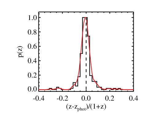
For the remaining sources in our sample with secure optical counterparts we adopt photometric redshifts from Ilbert et al. (2006), which are based on the CFHTLS data. The redshifts are based on template fitting and a Bayesian approach, and thus use the same method as the BPZ code. The priors are calibrated using spectroscopic identifications of galaxies in the D1 field of the CFHTLS. The estimates are less reliable than the ANN results (), but do provide redshift information for the remaining optically identified X-ray sources. However there is a systematic bias for sources with to be placed at lower redshifts, as was found for the CDF-S and CDF-N. The authors have made available the full redshift probability distributions for every source, which we have adopted to account for the uncertainties, though once again will not account for the systematic bias.
2.1.4 ASCA Large Sky Survey
The ASCA Large Sky Survey (Ueda et al., 1999, ALSS,) covers a contiguous area of deg2 near the north Galactic pole, and contains 34 sources detected in the hard (2–7 keV) band with the SIS detector, down to a flux limit (2–10 keV). Optical identifications have been presented by Akiyama et al. (2000). 2 of these sources are optically identified as galaxy clusters, 1 is a star and 30 are associated with AGN, all of which have spectroscopic redshifts. 1 source remains unidentified. An area curve for this survey was presented by Akiyama et al. (2003), which we adopt for our work. We note that this area curve does not fully account for the Poissonian nature of the X-ray source detection, but as a relatively high flux limit was set for the catalogue and the X-ray fluxes will be accurately measured this is unlikely to have an adverse affect on our bright end determination.
2.1.5 ASCA Medium Sensitivity Survey
The largest area survey in our study is the ASCA Medium Sensitivity Survey (Ueda et al., 2001, AMSS,). We include sources from the AMSSn sub-sample, selected in the hard (2–10 keV) band, with optical identifications presented by Akiyama et al. (2003). The sample includes 87 X-ray sources, 76 of which are AGN, to a flux limit of , and is 100% optically identified with spectroscopic redshifts available for all the AGN. We include additional sources with redshift identifications from the AMSSs sub-sample (Ueda & Akiyama, private communication), which includes 20 AGN; 2 sources in this sample remain unidentified. The area curve for the combined AMSSn and AMSSs samples was presented by Ueda et al. (2003).
2.2 High-redshift sample
Due to the catastrophic failure of our photometric redshift estimates at , we have also investigated an alternative colour pre-selection approach for identifying AGN at high-redshift, building on the work of Aird et al. (2008). We include four of the fields used in Aird et al. (2008): HDF-N (fully encompassed by the CDF-N X-ray field described above), LALA CETUS, Lynx and EGS1. We additionally include the large area covered by both the AEGIS-X survey and the CFHTLS field D3 optical imaging. This fully encompasses the GWS field used in Aird et al. (2008), and thus supersedes those data. Our high-redshift data overlaps with our hard X-ray selected samples described in section 2.1; in section 3.3 we explain how data from our hard X-ray surveys at and our high-redshift colour pre-selected samples are combined to determine the evolution of the XLF.
2.2.1 Optical data
The reduction of the optical data for HDF-N, LALA CETUS, Lynx and EGS1 and the source detection and photometry with SExtractor has been described in Aird et al. (2008) and Reddy et al. (2006), and we refer the reader to those papers for further details. For the CFHTLS we have used the publicly released images and catalogues available from Canada Astronomical Data Center22 2 http://www4.cadc-ccda.hia-iha.nrc-cnrc.gc.ca/community/CFHTLS-SG/docs/cfhtls.html, March 2008 release. The catalogues were generated using SExtractor, although with a slightly different configuration to Aird et al. (2008). Initial detection was performed in the -band (which is the deepest band), and magnitudes were determined in the other bands using the Kron (1980) style aperture (determined from the band data). The data were not smoothed to match the seeing in different bands. These differences will affect the detection of objects and measurements of their colours, although given the depth and quality of the CFHTLS data is unlikely to adversely affect the colour selection of candidates. Nevertheless, any errors, biases and scatter due to the source detection and photometry procedure will be accounted for by our simulations to derive the optical selection functions (section 3.3.1).
Samples of Lyman-Break Galaxies (LBGs) were extracted from the optical catalogues using the standard selection criteria from Steidel et al. (2003):
| (1) |
with the faint limit of for EGS1. An additional sample of objects at slightly lower redshifts is selected using the BX selection criteria (Adelberger et al., 2004)),
| (2) |
These objects are “sub-U dropouts”, falling in a thin slice of colour space below the Lyman-break criteria, with a selection function that peaks around .5 (see section 3.3.1).
Objects were selected from the CFHTLS optical data using the same criteria. However, there are significant differences between the CFHTLS filter set and our G filters used in the other fields. The -band falls between the and filters, thus total -band magnitudes were calculated for every object using an approximate colour correction, given by
| (3) |
which was determined from our model colour distributions described in section 3.3.1. These estimated -magnitudes were used to apply the total magnitude limits, consistent with our other fields. However, for the selection in colour-space we used the original magnitudes in place of G, thus avoiding the effects of uncertain colour-corrections. The differences in the filters will lead to different selection functions, which we determine in section 3.3.1.
| Field | RA | Dec | a | X-ray | Survey | Selection | d | e | f | g | h |
|---|---|---|---|---|---|---|---|---|---|---|---|
| name | exposureb | areac | |||||||||
| (J2000) | (J2000) | () | (ks) | (arcmin2) | |||||||
| HDF-N | 12:36:55 | +62:14:18 | 1.5 | 1862.9 | 149.1 | BX | 1192 | 9 | 8 | 2 | 7 |
| LBG | 292 | 3 | 2 | 0 | 3 | ||||||
| AEGIS-X/CFHTLS | 14:17:43 | +52:28:25 | 1.2 | 188.7 | 1155.6 | BX | 17050 | 77 | 26 | 10 | 66 |
| LBG | 6933 | 30 | 10 | 0 | 30 | ||||||
| Lynx | 08:48:56 | +44:54:50 | 1.0 | 186.5 | 243.4 | BX | 647 | 2 | 0 | 0 | 2 |
| LBG | 223 | 1 | 1 | 0 | 1 | ||||||
| EGS1 | 14:22:43 | +53:25:25 | 1.2 | 177.8 | 358.9 | BX | 809 | 8 | 0 | 0 | 7 |
| LBG | 329 | 7 | 0 | 0 | 7 | ||||||
| LALA CETUS | 02:04:44 | 05:05:34 | 2.2 | 173.1 | 233.3 | BX | 660 | 4 | 0 | 0 | 4 |
| LBG | 144 | 3 | 0 | 0 | 3 |
aGalactic column density from Dickey & Lockman (1990).
bX-ray exposure time after good time interval and background ßare Þltering (average of the individual pointings for AEGIS-X).
cTotal survey area covered by X-ray and optical data.
dNumber of candidates from the optical imaging satisfying the colour selection criteria.
eNumber of the colour-selected candidates with secure X-ray counterparts.
fNumber of the X-ray detected candidates with spectroscopic redshifts.
gNumber of the spectroscopically identified sample which are low redshift interlopers ().
2.2.2 X-ray data
All of our fields have been observed with Chandra, and have exposure times ks. The data have been reduced using our pipeline procedure (Laird et al., 2009). For our high-redshift samples we use sources detected in the soft-band with significance . Our colour pre-selection limits us to sources at , and at these redshifts the soft-band will probe rest-frame energies keV. Thus our selection should be relatively unbiased for the selection of moderately absorbed AGN ( cm-2), and is comparable with the hard-band selection employed at lower redshifts (Cowie et al., 2003; Barger et al., 2005).
2.2.3 Matching the X-ray and optical samples
We determined which of our colour pre-selected high-redshift objects host AGN by matching the optical and X-ray source lists. The matching is performed with the entire - (or -) selected optical catalogues using the likelihood ratio method. The colour selection criteria are then applied to the matches. Matching the entire optical catalogue ensures that X-ray sources are matched to the most likely optical counterparts, and prevents colour pre-selected objects being erroneously associated with nearby bright X-ray sources, which have correspondingly bright, secure optical counterparts (Aird et al., 2008, cf. the direct extraction method used in ).
In table 2 we list the total numbers of X-ray detected objects within each of our colour-selected samples. We searched for spectroscopic redshifts for our sources as described in sections 2.1.2 and 2.1.3 for the HDF-N and AEGIS-X fields respectively, and from Stern et al. (2002) for the Lynx field. Remaining unidentified sources were assigned redshift probability distributions, , based on the optical selection functions (see section 3.3.1).
2.2.4 Low-redshift interlopers
G LBG selection at is known to be extremely clean and contains very few low redshift interlopers (Steidel et al., 2003). The majority of interlopers are Galactic stars, which are not expected to be bright X-ray sources and thus will not contaminate our sample. However, the BX selection, which does not rely on very strong features such as the Lyman-break to identify candidates, is more susceptible to contamination from low-redshift sources, mainly from low-redshift () star-forming galaxies in which the Balmer-break is confused with the Lyman- forest absorption at (Adelberger et al., 2004; Reddy et al., 2006). Indeed, a significant number of low-redshift () interlopers are identified within our spectroscopically observed, X-ray detected BX sample (see table 2, Figure 3). By examining the positions of these sources in the plane (see Figure 4) it is clear that 5 of these low-redshift interlopers occupy a distinct position, associated with optically-bright objects (), but with relatively low X-ray fluxes, thus . These objects are the expected bright, low-redshift star-forming galaxies, with X-ray emission associated with star-formation processes. We exclude 2 more X-ray detected BX sources from our analysis which fall in the same region and are thus also suspected to be low-redshift contaminants. The faint BX source with and , which has a spectroscopic redshift in the correct range, is also excluded as we suspect a star-burst origin (Aird et al., 2008, see also).


The 6 remaining interlopers, however, are associated with low-redshift AGN, and thus fall within the AGN region . While any AGN which have been spectroscopically identified as low-redshift interlopers are excluded from our analysis, additional contaminants may remain within our unidentified BX sample. Based on our spectroscopic sample the fraction of low-redshift AGN contaminants may be as high as %, although our sample is biased in the sense that a higher fraction of bright objects have spectroscopic identifications. Indeed, in the large sample of BX-selected galaxies with spectroscopic redshifts used by Reddy et al. (2008) the low redshift contamination in the galaxy sample was % for bright candidates (), whereas for fainter candidates was only %. Conversely, in the sample of objects spectroscopically identified as AGN (including QSOs and narrow-line AGN), the contamination fraction was only %, and approximately consistent over the entire magnitude range. Clearly a much larger, near complete sample of spectroscopic redshifts for BX/X-ray selected AGN is required to truly determine the interloper fraction within our sample, and could also allow improvements to the selection criteria (such as introducing data from redder wavebands) to be developed to help reduce the contamination. However, given the current uncertainties, we have chosen not to make further corrections to account for the interloper fraction within our sample. We thus note that the faint end of our XLF based on the BX sample may be over estimated due to low-redshift contamination.
2.2.5 High luminosity sample
The total area coverage for our high-redshift sample remains relatively small, and thus we require an additional sample of high-luminosity AGN to constrain the bright end of the XLF. We have chosen to use bright objects ( ) from the Hasinger et al. (2005) compilation of surveys (excluding the CDF-N to avoid overlap with our own analysis). These samples provide a soft-band selected, highly complete, spectroscopically selected sample. We have included objects with , providing 30 high-luminosity AGN in our high-redshift sample. These bright, complete, spectroscopic surveys may be combined with our colour pre-selected samples by assuming a top-hat selection function over the chosen redshift range (see section 3.3.2).
3 A Bayesian approach to determine the XLF
Our compilation of X-ray surveys provides large samples of AGN over a range of redshifts with well-defined completeness, required to determine the evolution of the XLF. However, the faint sources from the Chandra fields are subject to uncertainty in both the redshift determination (for those sources with photometric redshifts or in the high- colour preselected samples) and the X-ray flux measurement (due to the small numbers of counts from the faintest sources). This has led us to develop a Bayesian methodology to make accurate inferences about the form and evolution of the XLF, accounting for the uncertainties in individual sources.
3.1 The likelihood function
The first step is to determine the likelihood function, , for which we have followed the work of Loredo (2004). Our individual sources are effectively Poissonian points, drawn from the distribution given by the XLF. Thus, for a given model XLF, the expected number of detectable sources, , is given by
| (4) |
where the integrals are taken over the entire range of possible values. is the area of the survey sensitive to a source of a particular luminosity, , and redshift, , and thus a particular flux if we assume a single spectral shape (power law with photon index ). effectively describes the probability of a source being detected. The luminosity function, , is the differential number density of sources per unit co-moving volume as a function of and , given an assumed model described by the set of parameters, . is the differential co-moving volume per unit area, as a function of .
As described in Loredo (2004), the likelihood function may be constructed from the product of the probabilities of the observed data from the individual sources, given the model, and the probability that no other objects were detected. For a Poisson process the probability of no objects being detected is simply . In the presence of individual source uncertainties, the probability of the observed data, , from an individual source , given the model XLF is found by marginalising over the model distribution of and . Thus,
| (5) | |||||
where represents the set of observed data from all sources, and the product in the second part of the equation is over detected sources. For the idealised situation where the redshift and luminosity are perfectly determined, will be a delta function at the true values, and equation 5 will generalise to the standard maximum likelihood estimator. For our sample is the convolution of the redshift probability distribution and the Poisson likelihood of obtaining the observed X-ray data, counts,
| (6) |
where is calculated from the hard band (2-10 keV) flux for a source of luminosity and redshift , assuming and Galactic . Thus the Poissonian nature of the counts from the X-ray sources, the associated uncertainty in the flux and the Eddington bias are naturally accounted for in our determination of the XLF. Assuming approximately corrects for absorption effects due to intrinsic column densities cm-2 at , although we have not chosen to make a more sophisticated correction on a source by source basis (see further discussion in section 5.2). Our approach builds on the work of Georgakakis et al. (2008), extended to include redshift information, and allows us to use the improved method of calculating the X-ray sensitivity. For sources with spectroscopic redshifts we assume delta functions for . We also assume delta functions for the luminosities of sources in both the hard and soft X-ray selected, large area, bright samples (sections 2.1.4, 2.1.5, and 2.2.5).
3.2 Correcting for incompleteness
The likelihood function above does not account for the incompleteness of our samples. In our hard X-ray selected samples, between % (AEGIS) and % (CDF-N, CDF-S) of the sources lack secure optical counterparts, and thus have neither spectroscopic nor photometric redshifts. However, we can derive a completeness correction term to account for the incompleteness in the likelihood function.
Figure 5(a) shows the distribution of the hard X-ray flux and optical magnitudes of our (optically identified) sources. Sources are scattered over a range of optical to X-ray flux ratios, approximately over the range although a small proportion are at lower ratios and a significant number of this hard X-ray selected sample exhibit . At faint X-ray fluxes, a large fraction will be unidentified due to their faint optical magnitudes. In Figure 5(b) we show the distribution of our sources. A Gaussian approximation, taking the sample mean, , and standard deviation, , is shown in red, and provides a reasonable description of this distribution. If we apply a strict magnitude limit of (sources fainter than this limit are now deemed unidentified), and assume that all the unidentified sources would have optical counterparts fainter than this limit (reasonable given the very deep optical data we have used to search for counterparts), then we can introduce a correction to the expected number of sources, , given by equation 4, based on the fraction of the distribution probed at a given flux. Thus,
| (7) | |||
where describes the -magnitude distribution of sources at a given flux, , and is derived from the Gaussian distribution of . is normalised such that
Thus the factor
| (8) |
is a completeness correction, reducing the expected number of detectable sources with low X-ray fluxes.

However, the observed distribution (the red curve in Figure 5) will be biased by the very incompleteness we are trying to correct for, as sources with will be missed. The extent of the bias will depend on the flux distribution of the X-ray sources (and thus the XLF, and the X-ray sensitivity), which determines the number of sources with faint X-ray fluxes where the problem arises. Therefore, to improve our completeness correction the distribution should be determined simultaneously with the XLF, accounting for the incompleteness, using the observed data (the -magnitudes of the detected sources). We therefore introduce into the second term in equation 5, modifying the likelihood to
| (9) | |||
where we neglect any uncertainty in the measurement of the -magnitude of an individual source, , which is a minor simplification. The parameters and are introduced as nuisance parameters, and will be determined along with the XLF, integrating over their uncertainties when making inferences regarding the XLF parameters, . In Figure 5b the green dashed line indicates the best-fit (mode) values of and for our LADE evolutionary model (section 4.2). The peak of the distribution is clearly shifted to a higher , indicating the bias in the simple estimates.
3.3 Incorporating the high- colour pre-selected samples
In section 4 we present results for the evolution of the XLF over the full available redshift range based on our hard X-ray selected sample only (using spectroscopic and photometric redshifts). However, due to the systematic bias in photo- estimates at , we also wish to derive the evolution using our high-redshift colour pre-selected samples. Due to the a priori colour selection these samples will suffer from large, but well-defined incompleteness. Accounting for this incompleteness, and combining our soft-band selected high- sample with the hard X-ray selected samples at lower redshifts requires a number of further modifications to our methodology.
3.3.1 Optical selection functions
The first step is to determine the optical selection functions for the colour selection criteria. These were determined using the simulation method described in Aird et al. (2008) (Steidel et al., 1999; Hunt et al., 2004; Reddy et al., 2008, see also). Three sets of template spectra were determined for different spectroscopic classifications (Steidel et al., 2003, QSO, NLAGN or GAL: see ), and used to generate model Gand colour distributions. GAL and NLAGN colours were generated using a Bruzual & Charlot (2003) model template spectrum for a galaxy with continuous star formation and age 1 Gyr. This template spectrum was reddened using the Calzetti et al. (2000) relation for obscuration by dust, with various extinction coefficients drawn from the distributions based on the observed range of UV spectral slopes for GAL and NLAGN sources in LBG samples (Adelberger & Steidel, 2000; Steidel et al., 2002; Steidel et al., 2003). Such modelling is not a full physical description for the NLAGN, being based only on a template spectrum for star-forming processes, but is sufficient to simulate the observed range of spectral shapes and redder distribution of broadband colours for NLAGN. For QSOs we have followed the work of Hunt et al. (2004). The template spectra were generated by varying the continuum slope and Ly equivalent widths of a composite of 59 QSO spectra (corrected for intergalactic absorption) from Sargent et al. (1989), based on the Gaussian distributions given in Hunt et al. (2004). These model spectra for all three types were then redshifted over the range and intergalactic absorption was applied by simulating a random line-of-sight to each object with intervening Lyman-limit absorption systems distributed according to the MC-NH model of Bershady et al. (1999), as described by Hunt et al. (2004). The final spectra are multiplied by the filter transmission curves to produce the model colour distributions. Figure 6 compares colours for a single model spectrum (for each classification) at different redshifts in both G and colour space.
The full colour distributions were used to add artificial objects into the optical imaging data. Selection functions are then determined as the probability of recovering an object with a given magnitude with either the LBG or BX selection as a function of redshift. Objects were recovered using our SExtractor routines (Aird et al., 2008, see ) in the G fields. The SExtractor configuration file used to generate the released catalogues for CFHTLS is available on-line33 3 http://www1.cadc-ccda.hia-iha.nrc-cnrc.gc.ca/community/CFHTLS-SG/docs/cfhtlscat.sex, thus we used this configuration for those data. Objects were selected in the -band image and flexible Kron (1980) style apertures were used to measure the magnitudes in other bands, and calculate the output colours. Our selection functions will thus account for the different source detection and photometry technique, and the effects of the different filter sets.

Figure 7 compares our final selection functions (derived from the simulations) for the different colour criteria, filter sets, and optical classifications. There are clear differences between the G and selections, which we expect given the varying wavelength coverage of the filter sets, and results in variation in our selection functions. The filter extends to longer wavelengths than the filter, and as such the colour becomes sensitive to the Lyman-break at higher redshifts than the G colour, as can be seen from the tracks in Figure 6. Thus the LBG selection functions are shifted to slightly higher redshifts when using rather than the G filter sets. The same effect leads to BX selection functions which probe to higher redshifts, although the low redshift cut-off is relatively unaffected. Thus the BX selection functions are generally broader for selection.
The red continuum of our NLAGN model generally leads to a reduced efficiency of the selection functions. This effect is particularly seen for the BX selection function for G colours. The example NLAGN model shown in Figure 6 has colours which are very close to the boundary of the BX selection box. The intrinsic scatter we apply to our models and the photometric scatter introduced via our simulations will both lead to incompleteness of the BX selection function, which is clearly seen in Figure 7 (bottom centre panel). However, the filter is significantly bluer than the bandpass, resulting in colours which are generally bluer than G, and thus the NLAGN BX selection function is less adversely affected by the red continuum for selection, and has a higher efficiency (cf. top and bottom central panels in Figure 7). The same effect is seen for the GAL BX selection functions, although is much milder as the distribution of GAL colours is not as red as the distribution of NLAGN colours.
The model tracks for the QSO colours in Figure 6 follow complicated routes which have very different shapes for the different filter sets. This is due the presence of the strong, broad emission lines, which will move in and out of the various filters at different redshifts. However, the basic characteristics necessary for our colour selections remain present: the Lyman-break leads to a rapid reddening of the G (or ) colour at ; a characteristically flat spectrum is found at lower redshifts.

3.3.2 Modifying the likelihood function
The optical selection functions described above can be used to modify the likelihood function derived in section 3.2, to allow us to combine the hard X-ray selected samples at low redshifts () and our colour pre-selected high-redshift samples. Firstly, , which effectively gives the probability of detecting a source with given and , must be modified to account for the 2 different selection techniques. For , is calculated from the area curves for our hard X-ray surveys, converting the hard (observed 2–10 keV) X-ray flux to an (rest-frame 2-10 keV) and assuming and Galactic , as before. For , we use the area as a function of soft X-ray flux, multiplied by the average of the combined BX and LBG selection functions, for all magnitudes and spectroscopic classifications for a field, scaled to a maximum of 1. Thus,
| (10) | |||||
| (11) |
where is the area of each field sensitive to a soft (0.5–2 keV) flux for a given 2–10 keV luminosity source at , assuming and Galactic , for each field. This reduces the probability of objects being detected outside of the range covered by the colour pre-selection, and thus provides realistic expected numbers at high redshifts in the likelihood evaluation (equation 9). As we consider the uncertainty in the X-ray flux we can utilise the method of Georgakakis et al. (2008) to determine the X-ray area curves. For the high luminosity sample (section 2.2.5), the equivalent selection function is simply a top-hat function over the entire redshift range (), corresponding to a complete spectroscopic follow-up of the purely X-ray selected high-luminosity sample.
For each of the individual colour-selected sources we must assume a redshift probability distribution, for which we adopt the selection function for the appropriate field and sample (unless a spectroscopic redshift is available in which case we adopt a delta function). Thus the differing redshift coverage of the selection criteria for different types and filter sets will provide some additional information regarding the evolution, and this effect will be explicitly accounted for by our study. The X-ray flux uncertainty is also accounted for in an identical manner as for the low-redshift hard-band selected samples, only converting from the soft-band flux to 2–10 keV rest-frame luminosities, to determine for each of our colour selected objects.
Additional weighting factors, , must also be introduced, which are added as exponents of the individual source likelihoods in equation 9. This factor serves two purposes. Firstly, it reduces the weight assigned to sources in our hard X-ray samples according to the fraction of their distribution which falls below .
| (12) |
Thus, sources will be assigned a weight of if they have a spectroscopic redshift , or if their based on the photo- estimate falls wholly below . Sources with or which is all above will be assigned a weight of 0 (effectively removing them). Sources with photo- estimates that span above and below will be given appropriate fractional weights.
For the colour pre-selected objects, is the ratio of the total co-moving volume sampled based on our estimate of the area curve (equation 11), and the the effective co-moving volume sampled, based on the selection function at the object’s magnitude.
| (13) |
where is the selection function for both BX and LBG selection for a field for the observed -magnitude. Thus for the high-redshift sample, the factors apply additional weight to sources with fainter optical magnitudes, which were thus less likely to be selected by the colour pre-selection technique.
Our colour-selected sources are also incorporated into the calculation of the distribution, and the subsequent completeness correction. The derived considers hard-band X-ray fluxes. To achieve this an equivalent hard-band flux is calculated for each , whereas for a source was originally derived from the observed soft-band flux. -band magnitudes are derived from the -magnitudes by applying a small colour correction (based on our model templates described above).
Sources identified as low-redshift interlopers (section 2.2.4) are excluded from the colour-selected samples, but may still be included in the main sample to constrain the XLF for the AEGIS and CDF-N fields where our surveys overlap. 34 sources which were assigned photometric redshifts in our original hard X-ray selected samples are also present in our BX or LBG samples. Of these 17 were assigned ; the remainder were assigned to the higher redshifts expected for objects in our colour selected samples. For all of these sources we do not consider the photo- distribution, and consider them solely with the colour selected samples, assigning the associated redshift distribution (based on the optical selection functions) and weighting factors.
3.4 Bayesian model comparison and parameter estimation
Having determined the likelihood function, our knowledge of the XLF can be fully described by the posterior probability function,
| (14) |
where we have introduced the symbol to represent a particular model hypothesis for the XLF, and is the prior probability we assign to values for the parameters , for model . The denominator, , is known as the Bayesian evidence, , and normalises the posterior.
There are now two tasks at hand. Firstly, we wish to determine the best estimates of the parameters, , for our model XLF, and assign them an error. Standard Monte-Carlo Markov Chain approaches can be used to draw samples from the posterior, and thus provide estimates of the parameters. Such approaches ignore the normalising factor, , as it is independent of the parameters. Our second task is to compare different evolutionary models. Bayesian model comparison is achieved by calculating the ratio of the posterior probabilities for different models (Kass & Raftery, 1995, e.g.),
| (15) |
where the ratio of the prior probabilities of the two different models, , can be taken as unity if we have no prior knowledge which indicates we should favour one of the models. The evidence can be calculated by integrating the likelihood over the prior parameter space, thus,
| (16) |
where represents the number of dimensions for the integration (i.e. the number of parameters, now incorporating the nuisance parameters and into the parameter set ). To perform this integration we have implemented the “nested sampling” algorithm (Skilling, 2004), which provides an estimate of the evidence, , along with a numerical uncertainty. 800 “live” objects are used for the nested sampling to ensure that the large, multi-dimensional parameter space is well sampled. Estimates of the posterior distribution may be recovered as a by-product of the nested sampling procedure, and thus used to determine the values of the parameters describing the XLF and their errors. We choose to report the posterior mode (equivalent to maximum likelihood) values of the parameters as our best estimates, and equivalent (68.3%) Highest Posterior Density (HPD) intervals, which minimise the size of the confidence interval for the given confidence level.
It is worth noting the difference of this Bayesian model comparison approach to frequentist methods. The frequentist approach to compare two models would be to calculate the likelihood ratio, the ratio of the maximum likelihood values for the two different models (Neyman & Pearson, 1928). The Bayesian approach, on the other hand, integrates the likelihood over the entire prior parameter space. As such the Bayesian evidence incorporates knowledge of all the uncertainties in the data and the parameter estimation. This approach also has the advantage that it naturally implements Occam’s Razor, favouring a simple model with a compact parameter space, thus less free parameters, over a more complicated one, unless the latter provides a significantly better description of the data (Berger & Jefferys, 1992).
3.5 Binned estimates
Our analysis of the evolution of the XLF considers each detected object individually, and does not require any binning. Our results consist of our best-fit parameter estimates and their uncertainties, and the relative Bayesian evidences for the different evolutionary models presented in section 4 and tables 3 and 4. However, for display purposes it is useful to produce binned estimates which represent the value and uncertainties over certain discreet ranges of luminosity and redshift. Our binned estimates are based on the method (Miyaji et al., 2001), which multiplies the value of the best-fit model evaluated at the centre of the bin by the ratio of the number of observed sources, , to the predicted number in the bin, , where
| (17) |
for each bin of size and . With our methodology a source is assigned a distribution of luminosities and redshifts, and thus can be included in multiple bins. Therefore the observed number of sources, , is found by summing the fractional contribution of all sources to each bin,
| (18) |
Errors on the binned values are based on approximate Poisson uncertainties on the effective number of objects in a bin. Points are only shown for bins with an effective .
4 Evolution of the XLF
We have used our Bayesian methodology and the nested sampling algorithm to compare three different evolutionary models of the XLF, using both our hard X-ray selected samples over all redshifts (using photometric and spectroscopic redshifts), and the combination of the hard X-ray sample at and the high-redshift colour pre-selected samples. For each evolutionary model we calculated the best-fit (mode) for the parameters, with errors given by the Highest Posterior Density interval, and the relative logarithmic evidence, . Differences in indicate very strong evidence in favour of the model with the higher evidence (Jeffreys, 1961). The results are given in tables 3 and 4 for the hard X-ray sample only and the combined samples respectively. Constant (or log-constant) priors were assumed for all parameters over the ranges indicated in table 3.
4.1 Evolutionary models
We compared the following evolutionary models:
4.1.1 Pure Luminosity Evolution (PLE)
At first we investigated models in which the XLF retains the same shape at all redshifts, but undergoes overall shifts in luminosity. We assume the standard double power-law shape for the XLF,
| (19) |
where is the faint-end slope, is the bright-end slope, is the characteristic break luminosity and is a normalisation factor for the overall density. Pure luminosity evolution can then be described as evolution of the characteristic luminosity, . Barger et al. (2005) found that the low redshift () XLF could be well described by a PLE model, where is given by
| (20) |
However, previous studies (Ueda et al., 2003; Silverman et al., 2008; Aird et al., 2008, e.g.) have indicated that the strong evolution of at low redshifts may not continue above . A number of authors have utilised models which extend equation 20 with additional quadratic or higher order terms in (Page et al., 1997; Silverman et al., 2008, e.g.). Alternatively, Ueda et al. (2003) described a PLE model which has 2 different slopes below and above a critical redshift, . This parameterisation allows the luminosity evolution to flatten off, cease completely, or increase or decline at high redshifts. We have adopted this form of luminosity evolution, additionally allowing for a smooth transition between the 2 slopes, thus the evolution of is given by
| (21) |
where the parameter controls the transition from the strong low- evolution to the high- form.
4.1.2 Luminosity and Density Evolution (LADE)
The work of Aird et al. (2008) indicated that while the XLF retained a similar shape at high redshift, there was an overall decline in the number density at the faint end (), yet little or positive evolution at the bright end. This behaviour cannot be described by PLE. We have modified the PLE form described above to additionally allow for some overall decreasing density evolution with redshift, by allowing the normalisation constant to evolve as
| (22) |
thus introducing an additional parameter, . With this parameterisation the shape of the XLF stays fixed at all redshifts, thus our evolution consists of an XLF which shifts in both luminosity and overall density. We refer to this evolutionary model as Luminosity And Density Evolution (LADE). This model is similar to the Independent Luminosity and Density Evolution (ILDE) described by Yencho et al. (2009), but with a different form for the density evolution and a more complex luminosity evolution that can flatten off at higher redshifts.
4.1.3 Luminosity-Dependent Density Evolution (LDDE)
As discussed in section 1, a number of authors have proposed that an evolutionary scheme in which the XLF undergoes a density evolution which is dependent on luminosity is required to accurately describe the evolution of both soft X-ray selected (Miyaji et al., 2000; Hasinger et al., 2005, e.g.) and hard X-ray selected (Ueda et al., 2003; Silverman et al., 2008, e.g.) AGN. We have adopted the parameterisation given by Ueda et al. (2003), in which a typical double power-law form (e.g. equation 19) of the XLF at is modified by an evolution term which is a function of luminosity and redshift,
| (23) |
where is a power-law function of , which changes between 2 different forms at a cut-off redshift, , which depends on the luminosity. Thus
| (24) |
where
| (25) |
We allow all the parameters to vary in our fitting (although apply priors over constant ranges), thus the evidence, , will fully account for the complexity of this parameterisation.
| Parameter | Lower limit a | Upper limit a | PLE | LADE | LDDE | |||||
| (or ) Mpc-3 | -7. | 0 | -3. | 0 | . | . | . | |||
| (or ) / | 43. | 0 | 46. | 0 | . | . | . | |||
| -0. | 1 | 1. | 5 | . | . | . | ||||
| 1. | 5 | 4. | 0 | . | . | . | ||||
| 3. | 0 | 10. | 0 | . | . | … | ||||
| -4. | 0 | 3. | 0 | . | . | … | ||||
| 2. | 0 | 6. | 0 | … | … | . | ||||
| -5. | 0 | 0. | 0 | … | … | . | ||||
| (or ) | 0. | 4 | 3. | 0 | . | . | . | |||
| -1. | 5 | 0. | 0 | … | . | … | ||||
| 44. | 0 | 46. | 0 | … | … | . | ||||
| 0. | 0 | 1. | 0 | … | … | . | ||||
| . | . | . | . | . | ||||||
aUpper and lower limits on the constant priors for the parameters.
4.2 Results
Table 3 gives the best-fit (posterior mode) parameters for our three evolutionary models using the hard X-ray selected samples only over all redshifts, and values of the Bayesian evidence relative to the evidence for the PLE model, . These values indicate the the LADE model, introducing an additional parameter, provides a significantly better fit than the PLE model. There is also very strong evidence favouring the more complicated LDDE parameterisation over either the LADE or PLE models. Figure 8 plots the maximum-likelihood LDDE model along with binned estimates for a range of redshifts. It immediately apparent that our LDDE model predicts a much milder evolution of the faint end of the XLF than the model presented by Silverman et al. (2008), with significantly less flattening of the faint-end slope. This is most likely due to our inclusion of objects with fainter optical magnitudes and correction for remaining incompleteness in the samples (see further discussion in section 5.1 below. However, the majority of the flattening of the faint-end slope we do observe is found at , precisely where our photometric redshifts become unreliable and prone to catastrophic failure, and thus this measurement of the faint end of the XLF will be biased. Therefore, we are unable to confidently rule out the PLE or LADE evolutionary models using the results from direct hard X-ray selection only.
In table 4 we present the results for the three evolutionary models using the colour pre-selected samples at high redshifts in addition to the hard X-ray samples at . The colour pre-selection approach restricts the sample to sources for which we can reliably estimate the redshift. This should therefore provide more robust measurements of the XLF at high-redshifts that are not subject to systematic biases due to catastrophic failure of photometric redshifts. The sample size is smaller and incomplete, but due to the well-defined selection functions we are able to correct for this incompleteness. We find strong evidence favouring the LADE or LDDE models over the PLE model. We can thus rule out this simplest model, consisting of an XLF which only evolves in luminosity without changing shape or moving in overall density, and is thus unable to reproduce the lack of evolution of the bright end of the XLF at high redshifts and the observed decline at fainter luminosities. However, there is only very weak evidence () favouring the most complex LDDE evolutionary scheme over the simpler LADE model in which the XLF retains the same shape at all redshifts. We therefore conclude that there is no significant evidence that an LDDE parameterisation, and the associated flattening of the faint-end slope, is required to describe the evolution of the XLF. Our LADE model, in which the XLF retains the same shape but shifts in both luminosity and density, is also able to adequately describe the observed evolutionary behaviour. Our best-fit LADE model indicates strong luminosity evolution takes place between and , but is consistent with a value of , indicating that the evolution of flattens off at high redshifts, and the evolutionary behaviour becomes dominated by the overall negative density evolution.
Our LADE model is plotted in Figure 9, evaluated at the centre of a number of redshift bins, along with binned estimates (see section 3.5) using both the hard X-ray samples and the high- colour pre-selected samples. The LADE model is in good agreement with the bright end of the XLF determined from the hard X-ray selected samples at (open circles, not used to constrain this model), but generally predicts a higher number density below , reflecting the systematic failure of the photometric redshifts in this regime. At our binned estimates from the colour pre-selection are systematically below the LADE best fit (although agree within ). Indeed, the binned data appear to indicate that the overall number density drops between and , but then rises again between and (none of our evolutionary models could describe such behaviour). However, it is more likely that this behaviour reflects additional incompleteness in the BX selection, which has not been accounted for. The issues and limitations of our methodology are discussed further in section 5.2 below. There is much better agreement with the binned estimates, where the sample is larger and the XLF is more robustly determined.


| Parameter | PLE | LADE | LDDE | |||
| (or ) Mpc-3 | . | . | . | |||
| (or ) / | . | . | . | |||
| . | . | . | ||||
| . | . | . | ||||
| . | . | … | ||||
| . | . | … | ||||
| … | … | . | ||||
| … | … | . | ||||
| (or ) | . | . | . | |||
| … | . | … | ||||
| … | … | . | ||||
| … | … | . | ||||
| . | . | . | ||||
5 Discussion
Our results for the evolution of the faint end of the 2–10 keV XLF should be the most accurate and robust to date. Our work utilises both of the Chandra deep fields, including the full 2 Ms exposure available for each field. The additional large area of deep (200 ks) X-ray data provided by the AEGIS survey are also essential for an accurate determination of the faint-end slope. Our sensitive point source detection techniques allow us to probe to the greatest depths in these data, yet our Bayesian techniques allow us to fully account for uncertainty in the flux measurements at these faint limits, and account for the Eddington bias. By incorporating photometric redshift estimates we are able to achieve high redshift completeness (%), but we have accounted for the uncertainty in such redshift determinations. We have corrected for remaining incompleteness in our samples using the relation between optical and X-ray fluxes, which we have constrained based on our observed samples. At high redshifts we use colour pre-selection to constrain the XLF and reduce biases due to the catastrophic failures of photo- estimates. We have also used a likelihood ratio matching technique to ensure we only include robust optical counterparts to X-ray sources.
5.1 Comparison with previous results
Our work offers a number of improvements over previous studies. No previous work has considered the errors in X-ray fluxes and detection threshold, and thus will not account for Eddington bias. Additionally, no prior studies utilising photometric redshifts (Barger et al., 2005; Silverman et al., 2008; Ebrero et al., 2009, e.g.) have accounted for the known uncertainties in such estimates, or the possible effects of catastrophic failures which we believe led to a biased result at high redshifts in our work (see Figure 8, section 4.2). The commonly used photometric redshift catalogue for the CDF-N, presented by Barger et al. (2003), used the same optical data as our work, and the BPZ code, and thus these estimates will be subject to the same uncertainties and potential for catastrophic failures. Zheng et al. (2004) used a range of photo- codes, incorporated a wider range of optical filters, deep HST imaging data, and used the X-ray data as an indication of absorption properties, to provide improved photometric redshift estimates of X-ray sources in the CDF-S (1 Ms data). Although these estimates were found to be accurate to within %, the authors discussed the remaining uncertainties, particularly for the fainter sources, and the possibility of catastrophic failure. The lack of spectroscopic follow-up makes it difficult to assess the reliability of all photometric redshifts at high-, and the uncertainties should be accounted for in estimates of the XLF.
Our completeness corrections allow us to account for the lack of redshift information for a fraction of our sources, which is particularly important for determining the faint end of the XLF, where the optical counterparts are often too faint to be detected in even the deepest available imaging. Previous authors have often omitted any form of completeness correction, instead setting high X-ray flux limits (Ueda et al., 2003, e.g.) or presenting maximal XLFs assigning all unidentified sources to a given redshift bin (Barger et al., 2005, e.g.). Silverman et al. (2008) did apply a completeness correction, based on the fraction of sources with a given X-ray flux with redshift information, although samples were restricted to objects with bright optical counterparts () which may introduce additional biases. Ebrero et al. (2009) restricted their analysis to samples with high-redshift identification completeness, and applied small additional corrections based on the fraction of identified sources as a function of X-ray flux, although the completeness was likely to be over estimated in the CDF-S as they did not consider the high fraction of spurious counterparts. A similar approach was adopted by Yencho et al. (2009), although their samples were restricted to spectroscopic identifications and thus these completeness corrections were large (%) at the faintest flux levels, and may be subject to additional biases and inaccuracies given the large number of complex factors involved in spectroscopic success rates. We thus believe our approach of considering only robust optical counterparts to X-ray sources and modelling the distribution of ratios, in addition to our colour pre-selection approach at high-redshifts, constitutes a more robust treatment of completeness than in previous work.
In Figure 10 we directly compare the evolution of the space density of AGN predicted by our LADE model and a number of recent studies of the evolution of the XLF, all of which concluded that LDDE was taking place. Results are shown in two luminosity bins, which approximately correspond to above and below the characteristic break luminosity, , although does evolve and thus such space density plots may provide a distorted view of the evolutionary behaviour of the XLF. Indeed, in the higher luminosity bin () our model indicates a very different evolution of the space density at to previous (LDDE) results, but this is partly due to small offsets in luminosity space which manifest as very large differences in density because of the steep slope of the bright end of the XLF. This can also lead to large differences in binned estimates depending on the methodology or assumed evolution of the XLF. However, in this regime, the XLF remains poorly constrained, and despite the very different evolutionary behaviour our binned results are consistent with the Silverman et al. (2008) and Ebrero et al. (2009) models at the level, although the Yencho et al. (2009) model is significantly lower. The high redshift form of our evolution in this luminosity bin predicts similar space densities to the previous studies, although the form of the evolution and location of the peak in the number density is somewhat different.
Our results are in good agreement at low redshifts () in the lower luminosity bin (), although the Yencho et al. (2009) results remain below our estimates. However, at higher redshifts our model predicts a much higher space density than found by Yencho et al. (2009) or Silverman et al. (2008). We attribute the decline found by these authors to incompleteness, catastrophic failures of photometric redshift estimates, and false associations of X-ray sources with lower redshift optical counterparts. Conversely, the Ebrero et al. (2009) LDDE model is in very good agreement with our result, most likely because of the higher completeness of their samples. However, our results have shown that an LDDE model is not necessary to describe this evolution.
It is worth noting that our LADE form of the evolution is able to describe a “cosmic-downsizing” behaviour in which the peak in the space density moves to lower redshifts for lower luminosity AGN, and indeed we do find small redshift offsets between the peak space densities for different luminosity ranges (e.g. Figure 10). However, our model does not find the strongly luminosity-dependent shift in peak space density indicated by some prior studies (Hasinger et al., 2005; Silverman et al., 2008, e.g.). This is mainly due to our steeper faint-end slope (and thus higher number density of low-luminosity AGN at ), but is also due to the differences in the form of the bright-end evolution discussed above.

5.2 Remaining uncertainties
While we believe our work offers a number of improvements over previous studies, there are remaining uncertainties associated with our approach.
5.2.1 Photometric redshifts
As previously discussed, the introduction of photometric redshifts, essential to improve the completeness of samples at faint X-ray fluxes, does introduce significant uncertainty, which we have tried to account for by considering probability distributions for the redshift estimates. However, there are a number of limitations to photometric redshift techniques that are thus also limitations in our studies. This is particularly apparent in the catastrophic failure of our photo- estimates at , which we believe led to a biased result for the evolution of the XLF, favouring an LDDE scheme with a flattening faint-end slope (section 4.2, table 3). Additionally, the majority of our photo- estimates are based on template fitting approaches that utilise a variety of galaxy templates (and priors based on the galaxy population), and thus the derived redshift probability distributions may not correspond to the true redshift for an AGN, which could bias our results at low as well as high redshifts. Incorporating AGN templates and using priors based on the AGN population may offer significant improvements and reduce systematic biases and catastrophic failures (Zheng et al., 2004; Salvato et al., 2008, e.g.). Expanding the number and wavelength range of the filters, such as including near- and far-IR data, also has potential to improve photometric redshift estimates and provide better fits to AGN templates (Salvato et al., 2008, e.g).
In addition to the template fitting approach, we also utilised ANN redshift estimates in the AEGIS field, in which an artificial neural network is trained to provide photometric redshifts using a sample of objects with spectroscopy. While this approach produced reliable results, it is limited to the subset of objects with a certain range of colours and magnitudes for which follow-up spectroscopy is available. Indeed, spectroscopic validation of photo- estimates for large numbers of optically-faint X-ray sources is impossible with current instrumentation, which is a major limitation of photometric redshift techniques.
5.2.2 High- colour pre-selection
To reduce the bias at high redshifts we incorporated rest-frame UV colour pre-selected samples. This should avoid the systematic biases associated with catastrophic failure of the photometric redshift estimates, but does risk introducing additional uncertainty and biases. As noted in section 4.2, the binned estimates based on the colour pre-selected samples at (dominated by BX selected objects) fell systematically below the model, ostensibly indicating a rise in the space density of AGN between and (also seen in Figure 10). The BX criteria select objects in a very thin slice of colour space, identifying objects with a specific spectral shape rather than strong spectral features. This makes the BX selection both more susceptible to contamination by lower redshift sources and more prone to incompleteness than the more widely-used LBG selection that identifies a strong break in the spectrum shortward of the Lyman-limit. The shape and efficiency of the derived selection functions will be highly dependent on the modelling of the AGN spectra and the scatter in their properties, and it is quite possible that our relatively simple modelling may have led to overestimates of the completeness. Indeed, both the LBG and BX selections require AGN to be bright in the rest-frame UV, and will therefore miss low-luminosity, moderately or heavily obscured AGN residing in red, evolved host galaxies. Aird et al. (2008) found that LBG selection recovered a number density of low-luminosity AGN that is at least as high as found via direct X-ray selection and follow-up, tentatively indicating that the AGN population at is dominated by objects with blue colours (Nandra et al., 2007, cf. ,). However, this may not be true at slightly lower redshifts, resulting in a lower number density at via the BX selection as red galaxies will be missed.
As discussed in section 2.2.4, our combination of LBG and X-ray selection to identify AGN does not suffer from low-redshift contamination, but this is not the case for the BX selection. Without complete spectroscopic follow-up of the X-ray detected BX candidates we cannot be confident that we have excluded all interlopers (although we believe we are able to identify low-redshift star-forming galaxies, see Figure 4), and it is unclear how this might affect our derived evolution of the XLF. Extensions of the BX selection technique, which incorporate data at redder wavelengths, may allow low-redshift interlopers to be excluded, and help identify AGN in redder host galaxies. Indeed, a hybrid of the photometric redshift and colour pre-selection approaches, utilising data from all available wavebands to perform SED fitting and estimate a redshift, but also performing a number of colour cuts to avoid catastrophic failures, and carefully modelling the distribution of AGN spectral properties to determine the incompleteness, may be the optimal approach to determine the high-redshift evolution.
It is also worth noting that our approach of combining direct hard X-ray selection at and colour pre-selection at high redshifts provides no data for . Significant evolution may be taking place over this redshift range, particularly at high luminosities (Silverman et al., 2005, e.g.). Indeed, at high luminosities incompleteness issues should be less severe, although we note that at we expect 10% of AGN with will have optical magnitudes , based on our distributions. In this redshift range, photometric redshift estimates are prone to catastrophic failure, and spectroscopic identification can also be difficult even for bright targets. Thus care must be taken to avoid biased results. As found in section 4.2, such systematic biases can erroneously indicate the need for a more complex evolutionary model.
5.2.3 Completeness corrections
To account for objects with optical magnitudes below our limit of , we introduced a simple completeness correction assuming the distribution can be described by the same Gaussian function at all redshifts (section 3.2). This may be an over simplification, as the redshift distribution of optically-faint sources will differ from the brighter population. Indeed, Mainieri et al. (2005) found that optically-faint X-ray sources tended to be found at higher redshifts. Additionally, Koekemoer et al. (2004) discuss how Extreme X-ray Objects (EXOs) which are X-ray bright but lack optical counterparts, even in very deep Hubble ACS imaging, may represent a population of very high-redshift () AGN where the redshifted Lyman-break suppresses all emission at optical wavelengths. More sophisticated modelling of the rest-frame UV–optical properties of the AGN population and the effects on observed magnitudes as a function of redshift would enable improvements to our completeness corrections. Furthermore, the shape and evolution of the optical luminosity function of the AGN host galaxies will affect the completeness of our samples , could alter the shape and efficiency of the optical selection functions, and may systematically impact the photo- estimates. In addition, we do not currently utilise any information from the optically-unidentified population (their X-ray fluxes, the fact that they lack counterparts to the limits of our imaging), which could place further constraints on the evolution of the XLF.
5.2.4 Cosmic variance
Our investigation of the XLF uses an unprecedented large area of deep 200 ks Chandra data in the AEGIS field, which supplements the data from the Chandra Deep Fields used in previous studies (Barger et al., 2005; Silverman et al., 2008, e.g.). As such, our determination of the faint-end evolution should be less susceptible to the effects of cosmic variance than in prior work. However, cosmic variance could introduce additional uncertainty in our XLF determinations (and thus weaken evidence for more complex evolutionary schemes). Indeed, assuming our X-ray detected AGN cluster according to a power-law with scale length Mpc and slope (Coil et al., 2009, typical of X-ray AGN at ), we predict a fractional RMS variation of % in the number density of AGN. This is comparable to our Poissonian uncertainties due to the number of objects in bin, although the errors will be basically covariant across the luminosity bins, and thus will not affect the shape of the XLF.
5.2.5 Intrinsic absorption
We have calculated rest-frame 2–10 keV luminosities for our sources from their hard band fluxes (or soft band for the high- sample), assuming a power-law with . This approach should correct for absorption effects due to intrinsic column densities of cm-2 at . However, the effectiveness of this correction varies with redshift, and this may bias our measurements of the luminosity, and alter the effective sensitivity of our observations. The extent of these effects will depend on the distribution of AGN absorption properties, which may be evolving with redshift or have a luminosity dependence (Ueda et al., 2003; La Franca et al., 2005). Some previous studies (Ueda et al., 2003; La Franca et al., 2005; Ebrero et al., 2009) instead attempted to correct for the effects of absorption on a source-by-source basis, and directly account for the distribution in their calculation of the XLF. Determining the extent of absorption is difficult for our faint sources, which have few counts and thus little X-ray spectral information. The effects of absorption on our X-ray sensitivity and completeness calculations will be complicated, and should be corrected for a number of potential selection biases . Such effects are in fact likely to introduce considerable additional uncertainty as to the evolution of the faint end of the XLF, and could thus strengthen our assertions of the lack of a requirement for a more complicated LDDE model to describe the evolution of the XLF. We defer these considerations to future work.
5.3 The evolution of AGN accretion activity
Our determination of the evolution of the XLF presented in this paper sheds new light on how the distribution of AGN accretion activity evolves over the history of the Universe. We conclude that given the currently available data, the evolution of the XLF can be described by a luminosity and density evolutionary scheme, in which the XLF retains the same shape, but shifts in both luminosity and density with redshift. A more complicated luminosity-dependent scheme does not provide a significantly better description of the data; even so our best-fit LDDE for the hard X-ray sample only, which we expect is biased at high redshifts, indicates a steeper faint-end slope and less evolution of the shape of the XLF than most previous work.
Hopkins et al. (2005) presented an interpretation of the AGN luminosity function in which the bright end traces the mass distribution of black-holes accreting at the peak rate over their lifetimes, while the faint end corresponds to AGN during transitionary periods as they approach or decline from their peak rate of activity. Furthermore, Hopkins et al. (2006) proposed that a luminosity-dependent lifetime for AGN could explain any observed flattening of the faint-end slope, as less time is spent in the transitionary period by the more luminous AGN found at high redshifts. Our results, however, show that the shape of the XLF does not change, thus a strongly luminosity-dependent lifetime may not be required. The lack of evolution in the shape of the XLF indicates the processes involved in the triggering and feeding of AGN remain the same at all redshifts, but increase in overall density from the earliest times until , and moving to lower luminosity systems between and the present day. Such behaviour could be consistent with a merger-driven model of the build-up of galaxy and black-hole mass, and the triggering of AGN (Kauffmann & Haehnelt, 2000; Hopkins et al., 2008, e.g.), in which the hierarchical build-up of galaxies increases the number density of AGN in the early history of the Universe, but the exhaustion of gas supplies in the most massive galaxies at later times (Cowie et al., 1996, e.g.) results in the “down-sizing” of AGN to lower luminosities. Fully reconciling such a picture with the full range of observational data for AGN, in addition to the observed evolution of galaxies, using current theoretical models clearly requires significant further investigation. Indeed a number of other processes may play a role in triggering and fuelling low luminosity AGN, such as minor mergers (Hernquist & Mihos, 1995), accretion of gas from a hot halo (Fabian & Rees, 1995) or bar-driven accretion (Sellwood & Moore, 1999). It is essential to assess the importance of such processes and understand the role they play in the evolution of AGN accretion activity.

In Figure 11 we plot the 2–10 keV luminosity density, , as a function of redshift, which provides a tracer of the total AGN accretion activity. The evolution of the total luminosity density for all AGN with is shown as well as the contribution of AGN in set luminosity ranges. The total luminosity density peaks at , rapidly declining to lower redshifts, but the decline to higher redshifts is much milder indicating significant AGN activity is taking place out to –4. AGN with luminosities in the range (i.e. ) are responsible for the majority of the luminosity density, although the contribution of AGN falls off rapidly at as evolves, and AGN dominate.
We can track the build-up of black-hole mass more directly by relating AGN luminosity to mass accretion, as first proposed by Soltan (1982),
| (26) |
where is the mass accretion rate, is the rate of change of black-hole mass density, is the bolometric luminosity, is the radiative efficiency of the accretion process and is the speed of light. We have adopted a simple approach (Barger et al., 2005, e.g.), converting our 2–10 keV X-ray luminosities to bolometric values using a constant conversion factor (Elvis et al., 1994, 40,), and assuming a single value of the radiative efficiency, (Marconi et al., 2004). We note that a number of authors have discussed the need for luminosity-dependent bolometric corrections (Marconi et al., 2004; Hopkins et al., 2007, e.g.), and Vasudevan & Fabian (2007) reported significant object to object variation in bolometric corrections, which may depend on the Eddington ratio. The radiative efficiency may also vary significantly between AGN, depending on the spin of the black-hole (Thorne, 1974, e.g.) in addition to the specifics of the accretion processes (Merloni & Heinz, 2008, e.g.). However our simple assumptions allow an initial investigation of the consequences of our derived XLF evolution on the build-up of black-hole mass. Using equation 26 we can convert our luminosity densities to a mass accretion rate, and thus calculate the total black-hole mass density as built up by accretion activity over the history of the Universe. Our results are shown in Figure 12.

Based on our LADE model we predict a local black-hole mass density of Mpc-3, where the error reflects the uncertainties in our model fit, but not the potentially larger uncertainties in bolometric correction or accretion efficiency. This value is in good agreement with the estimate of Yu & Tremaine (2002) ( Mpc-3) based on velocity dispersions of early-type galaxies in SDSS and the relation, although is lower than the estimate of Marconi et al. (2004) ( Mpc-3), possibly indicating that our XLF does not provide a complete census of the history of accretion activity. Figure 12 shows that a significant fraction (%) of this total mass density is accreted at . While the majority of the mass build up takes place in moderate luminosity AGN ( ), a significant fraction is accumulated at lower luminosities ( ). The LDDE model from section 4 predicts a lower local black-hole mass density, mainly due to the smaller numbers of AGN at these low luminosities and high redshifts. The redshift range –3 clearly corresponds to a period of significant AGN activity, and thus it is essential to accurately measure the XLF down to in this epoch to determine the history of black-hole mass accretion.
We can also compare our derived black-hole mass accretion rates to star-formation rates, which we show in Figure 13. Previous studies (Boyle & Terlevich, 1998; Silverman et al., 2008, e.g.) have shown close similarities between the rapid increase in star-formation rate and black-hole accretion at , which we confirm. Our results indicate that this correlation continues out to high redshifts (Silverman et al., 2008, cf.), at least when comparing to the recent star-formation rates of Bouwens et al. (2007), although we note that our model is extrapolated far beyond the redshift range probed by our data. Comparisons of the galaxy and AGN luminosity functions may reveal differences in the details of the evolving distributions of activity, which could reveal further facets of the co-evolutionary processes and the feedback regulating AGN activity and star-formation.

6 Summary
We have presented new observational determinations of the X-ray luminosity function of AGN. We utilised a hard X-ray selected sample from both the 2 Ms Chandra Deep Fields and the large area, deep 200 ks Chandra survey in the AEGIS field. A likelihood ratio method was employed to match X-ray sources to optical counterparts and ensure only robust associations were considered. To improve our redshift completeness, we supplemented spectroscopic identifications with photometric redshifts. However, we found our photo- estimates were systematically biased and prone to catastrophic failure at . We therefore adopted a rest-frame UV colour pre-selection approach to constrain the XLF at high redshifts. By carefully modelling the expected colour distributions of AGN, performing simulations of the optical data and repeating the source recovery procedure, we were able to determine well-defined selection functions that allowed us to correct for the incompleteness associated with the pre-selection technique.
We developed a sophisticated Bayesian methodology to determine the evolution of the XLF, which accounts for the uncertainties in photometric redshift estimates, the Poissonian nature of the X-ray flux estimate, the fraction of sources with counterparts below the magnitude limits of the optical data, and the optical selection functions at high redshifts. Using a Bayesian model comparison approach, we found that a Pure Luminosity Evolution was unable to adequately describe the evolution of the XLF, but a scheme in which the XLF evolves in both luminosity and density (LADE), but does not change shape, did provide a good fit. We did not find significant evidence for a more complex luminosity-dependent density evolution (LDDE), and the associated flattening of the faint-end slope. However, an LDDE model was required if the direct X-ray selected samples and the photometric redshift estimates were utilised at , but we believe such a result to be biased due to the inclusion of unreliable photo- estimates.
The form of our derived evolution of the XLF differs from many previous results (Silverman et al., 2008; Ebrero et al., 2009; Yencho et al., 2009, e.g.). Our XLF retains the same shape at all redshifts, which may have a number of consequences for the evolution of the black-hole mass function, AGN lifetimes and duty cycles, and the processes that fuel and trigger AGN. We find that the total luminosity density peaks at . While there is a mild decline at , significant AGN activity is still taking place at high redshifts. We find significantly higher number densities of low luminosity AGN ( ) at , which make a significant contribution to the to the total luminosity density and growth of black-hole mass at these redshifts. Our results do not indicate a strong shift of the peak space density to lower redshifts for lower luminosities, although a small shift is predicted by our best-fit evolutionary model. The mild decline in AGN activity to high redshifts appears to correlate with that seen in the star-formation rate, consistent with a co-evolutionary scheme for black-holes and galaxies.
Acknowledgements
We acknowledge financial support from STFC (JA, ESL). Some observations reported here were obtained at the MMT Observatory, a joint facility of the Smithsonian Institution and the University of Arizona. Also based in part on observations obtained with MegaPrime/MegaCam, a joint project of CFHT and CEA/DAPNIA, at the Canada-France-Hawaii Telescope (CFHT) which is operated by the National Research Council (NRC) of Canada, the Institut National des Sciences de l’Univers of the Centre National de la Recherche Scientifique (CNRS) of France, and the University of Hawaii. This work is based in part on data products produced at TERAPIX and the Canadian Astronomy Data Centre as part of the Canada-France-Hawaii Telescope Legacy Survey, a collaborative project of NRC and CNRS.
References
- Adelberger & Steidel (2000) Adelberger, K. L., & Steidel, C. C. 2000, ApJ, 544, 218
- Adelberger et al. (2004) Adelberger, K. L., Steidel, C. C., Shapley, A. E., Hunt, M. P., Erb, D. K., Reddy, N. A., & Pettini, M. 2004, ApJ, 607, 226
- Aird et al. (2008) Aird, J., Nandra, K., Georgakakis, A., Laird, E. S., Steidel, C. C., & Sharon, C. 2008, MNRAS, 387, 883
- Akiyama et al. (2000) Akiyama, M., et al. 2000, ApJ, 532, 700
- Akiyama et al. (2003) Akiyama, M., Ueda, Y., Ohta, K., Takahashi, T., & Yamada, T. 2003, ApJS, 148, 275
- Alexander et al. (2003) Alexander, D. M., et al. 2003, AJ, 126, 539
- Barger et al. (2003) Barger, A. J., et al. 2003, AJ, 126, 632
- Barger et al. (2005) Barger, A. J., Cowie, L. L., Mushotzky, R. F., Yang, Y., Wang, W.-H., Steffen, A. T., & Capak, P. 2005, AJ, 129, 578
- Barger et al. (2008) Barger, A. J., Cowie, L. L., & Wang, W.-H. 2008, ApJ, 689, 687
- Barmby et al. (2008) Barmby, P., Huang, J.-S., Ashby, M. L. N., Eisenhardt, P. R. M., Fazio, G. G., Willner, S. P., & Wright, E. L. 2008, ApJS, 177, 431
- Benítez (2000) Benítez, N. 2000, ApJ, 536, 571
- Berger & Jefferys (1992) Berger, J., & Jefferys, W. 1992, Statistical Methods and Applications, 1, 17
- Bershady et al. (1999) Bershady, M. A., Charlton, J. C., & Geoffroy, J. M. 1999, ApJ, 518, 103
- Bouwens et al. (2007) Bouwens, R. J., Illingworth, G. D., Franx, M., & Ford, H. 2007, ApJ, 670, 928
- Boyle et al. (1993) Boyle, B. J., Griffiths, R. E., Shanks, T., Stewart, G. C., & Georgantopoulos, I. 1993, MNRAS, 260, 49
- Boyle & Terlevich (1998) Boyle, B. J., & Terlevich, R. J. 1998, MNRAS, 293, L49
- Bruzual & Charlot (2003) Bruzual, G., & Charlot, S. 2003, MNRAS, 344, 1000
- Calzetti et al. (2000) Calzetti, D., Armus, L., Bohlin, R. C., Kinney, A. L., Koornneef, J., & Storchi-Bergmann, T. 2000, ApJ, 533, 682
- Capak et al. (2004) Capak, P., et al. 2004, AJ, 127, 180
- Ciliegi et al. (2003) Ciliegi, P., Zamorani, G., Hasinger, G., Lehmann, I., Szokoly, G., & Wilson, G. 2003, A&A, 398, 901
- Coil et al. (2009) Coil, A. L., et al. 2009, ArXiv e-prints
- Coleman et al. (1980) Coleman, G. D., Wu, C.-C., & Weedman, D. W. 1980, ApJS, 43, 393
- Collister & Lahav (2004) Collister, A. A., & Lahav, O. 2004, PASP, 116, 345
- Cowie et al. (1996) Cowie, L. L., Songaila, A., Hu, E. M., & Cohen, J. G. 1996, AJ, 112, 839
- Cowie et al. (2003) Cowie, L. L., Barger, A. J., Bautz, M. W., Brandt, W. N., & Garmire, G. P.
- Davis et al. (2007) Davis, M., et al. 2007, ApJ, 660, L1
- Dickey & Lockman (1990) Dickey, J. M., & Lockman, F. J. 1990, ARA&A, 28, 215
- Dickinson et al. (2003) Dickinson, M., Giavalisco, M., & The Goods Team. 2003, in The Mass of Galaxies at Low and High Redshift, ed. R. Bender & A. Renzini, 324–+
- Ebrero et al. (2009) Ebrero, J., et al. 2009, A&A, 493, 55
- Elvis et al. (1994) Elvis, M., et al. 1994, ApJS, 95, 1
- Fabian & Rees (1995) Fabian, A. C., & Rees, M. J. 1995, MNRAS, 277, L55
- Georgakakis et al. (2008) Georgakakis, A., Nandra, K., Laird, E. S., Aird, J., & Trichas, M. 2008, MNRAS, 388, 1205
- Giacconi et al. (2002) Giacconi, R., et al. 2002, ApJS, 139, 369
- Hasinger et al. (2005) Hasinger, G., Miyaji, T., & Schmidt, M. 2005, A&A, 441, 417
- Hernquist & Mihos (1995) Hernquist, L., & Mihos, J. C. 1995, ApJ, 448, 41
- Hopkins (2004) Hopkins, A. M. 2004, ApJ, 615, 209
- Hopkins et al. (2005) Hopkins, P. F., Hernquist, L., Cox, T. J., Di Matteo, T., Robertson, B., & Springel, V. 2005, ApJ, 630, 716
- Hopkins et al. (2008) Hopkins, P. F., Hernquist, L., Cox, T. J., & Kereš, D. 2008, ApJS, 175, 356
- Hopkins et al. (2006) Hopkins, P. F., Hernquist, L., Cox, T. J., Robertson, B., Di Matteo, T., & Springel, V. 2006, ApJ, 639, 700
- Hopkins et al. (2007) Hopkins, P. F., Richards, G. T., & Hernquist, L. 2007, ApJ, 654, 731
- Hunt et al. (2004) Hunt, M. P., Steidel, C. C., Adelberger, K. L., & Shapley, A. E. 2004, ApJ, 605, 625
- Ilbert et al. (2006) Ilbert, O., et al. 2006, A&A, 457, 841
- Jeffreys (1961) Jeffreys, H. 1961, Theory of probability (Clarendon Press)
- Kass & Raftery (1995) Kass, R. E., & Raftery, A. E. 1995, Journal of the American Statistical Association, 90, 773
- Kauffmann & Haehnelt (2000) Kauffmann, G., & Haehnelt, M. 2000, MNRAS, 311, 576
- Kinney et al. (1996) Kinney, A. L., Calzetti, D., Bohlin, R. C., McQuade, K., Storchi-Bergmann, T., & Schmitt, H. R. 1996, ApJ, 467, 38
- Koekemoer et al. (2004) Koekemoer, A. M., et al. 2004, ApJ, 600, L123
- Kron (1980) Kron, R. G. 1980, ApJS, 43, 305
- La Franca et al. (2005) La Franca, F., et al. 2005, ApJ, 635, 864
- Laird et al. (2009) Laird, E. S., et al. 2009, ApJS, 180, 102
- Le Fèvre et al. (2004) Le Fèvre, O., et al. 2004, A&A, 428, 1043
- Loredo (2004) Loredo, T. J. 2004, in American Institute of Physics Conference Series, Vol. 735, American Institute of Physics Conference Series, ed. R. Fischer, R. Preuss, & U. V. Toussaint, 195–206
- Luo et al. (2008) Luo, B., et al. 2008, ArXiv e-prints, 806
- Madau (1995) Madau, P. 1995, ApJ, 441, 18
- Mainieri et al. (2005) Mainieri, V., et al. 2005, A&A, 437, 805
- Marconi et al. (2004) Marconi, A., Risaliti, G., Gilli, R., Hunt, L. K., Maiolino, R., & Salvati, M. 2004, MNRAS, 351, 169
- Merloni & Heinz (2008) Merloni, A., & Heinz, S. 2008, MNRAS, 388, 1011
- Mignoli et al. (2005) Mignoli, M., et al. 2005, A&A, 437, 883
- Miyaji et al. (2000) Miyaji, T., Hasinger, G., & Schmidt, M. 2000, A&A, 353, 25
- Miyaji et al. (2001) —. 2001, A&A, 369, 49
- Mobasher et al. (2004) Mobasher, B., et al. 2004, ApJ, 600, L167
- Nandra et al. (2007) Nandra, K., et al. 2007, ApJ, 660, L11
- Nandra et al. (2005) —. 2005, MNRAS, 356, 568
- Neyman & Pearson (1928) Neyman, J., & Pearson, E. S. 1928, Biometrika, 20A, 175
- Page et al. (1997) Page, M. J., Mason, K. O., McHardy, I. M., Jones, L. R., & Carrera, F. J. 1997, MNRAS, 291, 324
- Popesso et al. (2008) Popesso, P., et al. 2008, ArXiv e-prints, 802
- Ravikumar et al. (2007) Ravikumar, C. D., et al. 2007, A&A, 465, 1099
- Reddy et al. (2006) Reddy, N. A., Steidel, C. C., Erb, D. K., Shapley, A. E., & Pettini, M. 2006, ApJ, 653, 1004
- Reddy et al. (2008) Reddy, N. A., Steidel, C. C., Pettini, M., Adelberger, K. L., Shapley, A. E., Erb, D. K., & Dickinson, M. 2008, ApJS, 175, 48
- Salvato et al. (2008) Salvato, M., et al. 2008, ArXiv e-prints, 809
- Sargent et al. (1989) Sargent, W. L. W., Steidel, C. C., & Boksenberg, A. 1989, ApJS, 69, 703
- Sellwood & Moore (1999) Sellwood, J. A., & Moore, E. M. 1999, ApJ, 510, 125
- Silverman et al. (2005) Silverman, J. D., et al. 2005, ApJ, 624, 630
- Silverman et al. (2008) —. 2008, ApJ, 679, 118
- Skilling (2004) Skilling, J. 2004, in AIP Conference Proceedings of the 24th International Workshop on Bayesian Inference and Maximum Entropy Methods in Science and Engineering, Vol. 735, 395–405
- Soltan (1982) Soltan, A. 1982, MNRAS, 200, 115
- Steidel et al. (1999) Steidel, C. C., Adelberger, K. L., Giavalisco, M., Dickinson, M., & Pettini, M. 1999, ApJ, 519, 1
- Steidel et al. (2003) Steidel, C. C., Adelberger, K. L., Shapley, A. E., Pettini, M., Dickinson, M., & Giavalisco, M. 2003, ApJ, 592, 728
- Steidel & Hamilton (1993) Steidel, C. C., & Hamilton, D. 1993, AJ, 105, 2017
- Steidel et al. (2002) Steidel, C. C., Hunt, M. P., Shapley, A. E., Adelberger, K. L., Pettini, M., Dickinson, M., & Giavalisco, M. 2002, ApJ, 576, 653
- Stern et al. (2002) Stern, D., et al. 2002, AJ, 123, 2223
- Sutherland & Saunders (1992) Sutherland, W., & Saunders, W., 1992, MNRAS, 259, 413
- Szokoly et al. (2004) Szokoly, G. P., et al. 2004, ApJS, 155, 271
- Thorne (1974) Thorne, K. S. 1974, ApJ, 191, 507
- Trouille et al. (2008) Trouille, L., Barger, A. J., Cowie, L. L., Yang, Y., & Mushotzky, R. F. 2008, ApJS, 179, 1
- Ueda et al. (2003) Ueda, Y., Akiyama, M., Ohta, K., & Miyaji, T. 2003, ApJ, 598, 886
- Ueda et al. (2001) Ueda, Y., Ishisaki, Y., Takahashi, T., Makishima, K., & Ohashi, T. 2001, ApJS, 133, 1
- Ueda et al. (1999) Ueda, Y., et al. 1999, ApJ, 518, 656
- Vanzella et al. (2008) Vanzella, E., et al. 2008, A&A, 478, 83
- Vasudevan & Fabian (2007) Vasudevan, R. V., & Fabian, A. C. 2007, MNRAS, 381, 1235
- Weiner et al. (2006) Weiner, B. J., et al. 2006, ApJ, 653, 1027
- Wolf et al. (2004) Wolf, C., et al. 2004, A&A, 421, 913
- Yencho et al. (2009) Yencho, B., Barger, A. J., Trouille, L., & Winter, L. M. 2009, ArXiv e-prints
- Yu & Tremaine (2002) Yu, Q., & Tremaine, S. 2002, MNRAS, 335, 965
- Zheng et al. (2004) Zheng, W., et al. 2004, ApJS, 155, 73