Baryon magnetic moments in large-$N_{c}$ chiral perturbation theory

From the theoretical point of view, the study of the magnetic moments of baryons presents an opportunity to shed light on an accurate test of QCD in the same way the magnetic moments of the electron and muon provided an accurate test of QED in the past. There are an important number of works focused on the analysis of baryon magnetic moments; the approaches include, among others, the quark model (and its variants) [1, 2, 3, 4, 5, 6, 7], QCD sum rules [8, 9, 10, 11], the $1/N_{c}$ expansion, where $N_{c}$ is the number of colors [12, 13, 14, 15], chiral perturbation theory [16, 17, 18, 19, 20, 21, 22, 23, 24, 25, 26], and lattice gauge theory [27], to name but a few. The $1/N_{c}$ expansion and chiral perturbation theory, on general grounds, have had a major impact on the extraction of the low-energy consequences of QCD.

On the one hand, the generalization of QCD from $N_{c}=3$ to $N_{c}\gg 3$ colors, referred to as the large-$N_{c}$ limit, provides a framework for studying the nonperturbative QCD dynamics of hadrons. Specifically, in the large-$N_{c}$ limit, the baryon sector of QCD possesses an exact contracted SU($2N_{f}$) spin-flavor symmetry, where $N_{f}$ is the number of light quark flavors [28, 29]. The spin-flavor structure for baryons for finite $N_{c}$ is thus given by analyzing $1/N_{c}$ corrections to the large-$N_{c}$ limit [28, 29]. Apart from the calculation of baryon magnetic moments, the $1/N_{c}$ expansion has also been successfully used in the calculation of other static properties of baryons such as masses [30, 28, 29, 31] and vector and axial-vector couplings [28, 29, 13, 33, 32]. Most calculations include corrections of relative order $1/N_{c}^{2}$, and even of relative order $1/N_{c}^{3}$ in the case of baryon masses, for two and three light quark flavors. The impact of the $1/N_{c}$ expansion in the calculation of baryon static properties can be assessed by comparing its predictions with experiment, which are in overall good agreement.

On the other hand, heavy baryon chiral perturbation theory [34, 35] is another formalism that has been implemented to systematically compute the properties of baryons. In this formalism, the expansion of the baryon chiral Lagrangian is in powers of $m_{q}$ and $1/M_{B}$, where $M_{B}$ is the baryon mass (for a recent review on chiral perturbation theory see for instance Ref. [36]). The effective Lagrangian thus obtained can be used to compute chiral logarithms in the effective theory, yielding to a remarkable computational simplicity because there are no gamma matrices left. One of the earliest applications of heavy baryon chiral perturbation theory can be found in the computation of one-loop corrections to the leading axial-vector couplings in baryon semileptonic decays [34, 35]. An important result derived from this analysis was the observation of large cancellations in the loop corrections between graphs with intermediate spin-1/2 octet and spin-3/2 decuplet baryon states. These cancellations occur as a consequence of the spin-flavor symmetry which is present in the large-$N_{c}$ limit, and have already been proven both phenomenologically and analytically [29, 13, 38, 37].

A further theoretical improvement has been achieved through a combined expansion in $1/N_{c}$ and chiral corrections [39, 40, 41], which can constrain the low-energy interactions of baryons with the meson nonet more effectively than either approach alone. In particular, in Ref. [41] a $1/N_{c}$ expansion of the chiral Lagrangian for baryons was proposed and applied to the calculation of the flavor-27 nonanalytic meson-loop corrections to the baryon masses. A more recent application of this formalism can be found in the renormalization of the baryon axial-vector current [37].

The earliest attempts of computing corrections to baryon magnetic moments beyond tree level in chiral perturbation theory can be traced back to the works of Caldi and Pagels [16], Gasser, Sainio and Svarc [17] and Krause [18]. Relatively more recent analyses can be found in Refs. [19, 21, 22, 23, 24, 25, 26].

The one-loop corrections to baryon magnetic moments have leading nonanalytic dependences on the quark masses and fall into two classes, namely, $m_{q}^{1/2}$ and $m_{q}\ln m_{q}$. Caldi and Pagels [16] focused on calculating what were supposed to be the leading corrections, namely, those of order $m_{s}^{1/2}$, and concluded that, in general, the corrections turned out to be at least as large as the zeroth-order contribution so that the perturbation expansion would break down. In turn, Gasser et. al. [17] reanalyzed these corrections whereas Krause [18] dealt with the logarithmic term, namely, $m_{s}\ln m_{s}$. Afterwards, Jenkins et. al. [19] reexamined the problem in the framework of heavy baryon chiral perturbation theory, including explicitly contributions of both intermediate octet and decuplet baryon states. Contrary to expectations, it was found that the inclusion of the decuplet did not produce appreciably better agreement with the data than the case when only the octet was included. In other words, the large cancellations observed in the one-loop corrections to the baryon axial-vector current when both octet and decuplet intermediate baryon states are included would not occur in the magnetic moments. It was argued that there could be some evidence that chiral perturbation theory overestimated the size of the kaon loops so it was proposed compensating such an effect by using the one-loop corrected axial-vector couplings rather than the tree-level ones.

Meissner and Steininger [21] also tackled the problem in the context of heavy baryon chiral perturbation theory but included all the terms up to order $\mathcal{O}(q^{4})$. They thus took into account $1/M_{B}$ corrections and contributions of certain double derivative operators which occur to this order. They however did not include the decuplet explicitly in the analysis; rather, its effects were considered by computing its contributions to some low-energy constants. Durand and Ha [22], in turn, performed the calculation in the same context of Ref. [19], emphasizing the role of the decuplet-octet mass difference; they found that there was not clear evidence of the convergence of the chiral series. Puglia and Ramsey-Musolf [23] performed an analysis similar to the one of Ref. [21], but included the decuplet explicitly and retained only nonanalytic one-loop corrections. Finally, Geng et. al. [25, 26], using covariant perturbation theory, found small loop corrections leading to an improvement over the SU(3) description.

All in all, the analyses performed over the past decade and a half about baryon magnetic moments have yielded a number of interesting conclusions, some of them in contradiction with the others. We would like to highlight, however, the role the decuplet plays as an intermediate state in the one-loop graphs.

In the present paper, we will confine our attention to the calculation of baryon magnetic moments in a simultaneous expansion in $m_{q}$ and $1/N_{c}$ at one-loop order. The starting point will be the fact that, in the large-$N_{c}$ limit, the baryon magnetic moment and the baryon axial-vector current share the same kinematical properties so that they can be described in terms of the same operators. Thus, for the main aim of the analysis we will use the formalism introduced in Ref. [41] and follow a close parallelism with the analysis of Ref. [37]. In this latter reference, the axial-vector form factor $g_{A}$, which enters into play in baryon semileptonic decays, was computed at one-loop order and compared, for $N_{f}=3$ and at the physical value $N_{c}=3$, with the corresponding one obtained in the framework of conventional heavy baryon chiral perturbation theory, i.e., the effective field theory with no $1/N_{c}$ expansion. The agreement observed, order by order, was remarkable.

We need to point out that, in Ref. [40], a similar analysis within the combined expansion has already been performed, based on the formulation implemented in Ref. [39], so we will pin down the similarities and/or differences of this approach with ours.

We have organized this paper as follows. In Sec. II we provide in broad terms an overview of the formalism on large-$N_{c}$ baryons in order to bring out the essential features of it. Our notation and conventions will be introduced accordingly. In Sec. III we construct the $1/N_{c}$ expansion of the baryon magnetic moment operator and then use it to obtain the tree-level values of the magnetic moments of the octet and decuplet baryons and the allowed octet-octet and decuplet-octet transitions. A total of 27 magnetic moments are obtained at this level. In Sec. IV we turn to the computation of one-loop nonanalytic corrections of the types $m_{q}^{1/2}$ and $m_{q}\ln m_{q}$, to relative order $\mathcal{O}(1/N_{c}^{3})$. In Sec. V we compare the results obtained in the combined expansion with the ones obtained in the framework of heavy baryon chiral perturbation theory. The comparison is carried out by establishing the relations existing between the parameters of the $1/N_{c}$ expansion and the invariant couplings of the chiral expansion. We devote Sec. VI to performing a detailed numerical comparison of our expressions with the available experimental data [42] by means of a least-squares fit. The best-fit parameters are then used to make some predictions of the unmeasured magnetic moments. Finally, in Sec. VII we present a summary as well as the main conclusions of the study. We complement the paper with two appendices which contain the reduction of all the baryon operators that appear to relative order $\mathcal{O}(1/N_{c}^{3})$, for $N_{f}$ and $N_{c}$ arbitrary.

For a detailed outline of the formalism on large-$N_{c}$ baryons and all the mathematical groundwork, which contains a formidable amount of group theory, we refer to the original works [28, 29, 41], while we restrict us here to a short description of the method and to introduce our notation and conventions.

First of all, the static baryon matrix elements of a QCD operator have a $1/N_{c}$ expansion of the form [29]

where the various $\mathcal{O}_{n}$’s are independent operators which transform according to the same spin$\otimes$flavor representations as $\mathcal{O}_{\mathrm{QCD}}$. For finite $N_{c}$, the sum on $n$ in Eq. (1) is over $0\leq n\leq N_{c}$ so that a given $\mathcal{O}_{n}$ is termed an $n$-body operator, which can be written as a monomial of degree $n$ in the baryon spin-flavor generators. On the other hand, each unknown operator coefficient $d_{n}(1/N_{c})$ has an expansion in $1/N_{c}$ beginning at order unity. The factor $1/N_{c}^{n}$ is required since each spin-flavor generator in an $n$th-order operator product $\mathcal{O}_{n}$ comes along with a factor of $1/N_{c}$. Additionally, the overall factor of $N_{c}$ arises because a QCD 1-body operator has matrix elements that are at most of order $\mathcal{O}(N_{c})$ when inserted on all quark lines on the baryon [29].

Specifically, for $N_{f}=3$, the large-$N_{c}$ spin-flavor symmetry for baryons is generated by the baryon spin, flavor and spin-flavor operators $J^{k}$, $T^{c}$ and $G^{kc}$, respectively, which can be written for large but finite $N_{c}$ as 1-body quark operators acting on the $N_{c}$-quark baryon states [29] as

where $q_{\alpha}^{\dagger}$ and $q_{\alpha}$ are operators that create and annihilate states in the fundamental representation of SU(6) and the index $\alpha$ sums over the $N_{c}$ quarks. In addition, $\sigma^{k}$ and $\lambda^{c}$ are the Pauli spin and Gell-Mann flavor matrices, respectively, where the spin index $k$ runs from one to three and the flavor index $c$ runs from one to eight. Throughout this paper, unless explicitly noticed otherwise, the square of the spin operator is given by $J^{2}\equiv J^{r}J^{r}$, where the ordinary convention of summing over repeated indices is adopted. No confusion is expected to arise from this. Without loss of generality, the baryon matrix elements of the spin-flavor generators (2) can be taken as the values in the nonrelativistic quark model, so this convention is usually referred to as the quark representation in the literature [29].

Analyzing the $N_{c}$ dependence of operator products appearing in the $1/N_{c}$ expansion (1) is not an easy matter due to the fact that the operator matrix elements have a different $N_{c}$ dependence in different parts of the flavor weight diagrams [29]. The $N_{c}$ dependence of the operator products is ultimately obtained by analyzing the $N_{c}$ dependence of the matrix elements of the baryon spin-flavor generators $J^{k}$, $T^{c}$, and $G^{kc}$ in the weight diagrams for the SU(3) flavor representations of the spin-1/2 and spin-3/2 baryons. In Ref. [38], a naive $1/N_{c}$ counting rule was implemented. However, on a more detailed level, baryons with spins of order unity have matrix elements of the flavor generators $T^{c}$ that are $\mathcal{O}(1)$, $\mathcal{O}(\sqrt{N_{c}})$, and $\mathcal{O}(N_{c})$ for $c=1,2,3$, $c=4,5,6,7$, and $c=8$, respectively, and matrix elements of the spin-flavor generators $G^{kc}$ that are $\mathcal{O}(1)$, $\mathcal{O}(\sqrt{N_{c}})$, and $\mathcal{O}(N_{c})$ for $c=1,2,3$, $c=4,5,6,7$, and $c=8$, respectively. Thus, factors of $T^{c}/N_{c}$ and $G^{kc}/N_{c}$ are of order 1 somewhere in the weight diagram, whereas factors of $J^{k}/N_{c}$ are of order $1/N_{c}$ everywhere [29].

As an illustrative example of the $1/N_{c}$ expansion for a baryon operator, let us consider the baryon axial-vector current $A^{kc}$, which is a spin-1 object, an octet under SU(3), and odd under time reversal. The $1/N_{c}$ expansion of $A^{kc}$ can thus be written as [29]

where $a_{1}$, $b_{n}$, and $c_{n}$ are unknown coefficients. The $\mathcal{D}_{n}^{kc}$ are diagonal operators with nonvanishing matrix elements only between states with the same spin, and the $\mathcal{O}_{n}^{kc}$ are purely off-diagonal operators with nonvanishing matrix elements only between states with different spin. The first few terms in expansion (3) read

whereas successive higher order operators are obtained as $\mathcal{D}_{n}^{kc}=\{J^{2},\mathcal{D}_{n-2}^{kc}\}$ and $\mathcal{O}_{n}^{kc}=\{J^{2},\mathcal{O}_{n-2}^{kc}\}$ for $n\geq 4$. The operators $\mathcal{O}_{m}^{kc}$, for $m$ even, are forbidden in expansion (3) because they are even under time reversal. At the physical value $N_{c}=3$ the series can be truncated as

The matrix elements of the space components of $A^{kc}$ between SU(6) baryon symmetric states yield the actual values of the axial-vector couplings. For octet baryons, the axial-vector couplings are $g_{A}$ as usually defined in baryon semileptonic decay experiments. After renormalization, $g_{A}\approx 1.27$ [37] for neutron $\beta$-decay.

The static properties of baryons can be determined from their couplings to the weak and electromagnetic currents. In particular, in this work, we will describe the magnetic moments in the context of large-$N_{c}$ chiral perturbation theory.

In the large-$N_{c}$ limit, the baryon magnetic moments possess the same kinematical properties as the baryon axial-vector couplings; as a result, the operators used to describe these quantities are practically identical [13]. The baryon magnetic moment operator, likewise the baryon axial-vector current operator $A^{kc}$, is a spin-1 object and an octet under SU(3). We will thus follow a close parallelism with the analysis of the renormalization of $A^{kc}$ performed in Ref. [37] in order to achieve our goal.

For definiteness, in analogy with Eq. (8), we construct the $1/N_{c}$ expansion of the operator which yields the baryon magnetic moment as follows

where we have truncated the series at the physical value $N_{c}=3$. If we assume SU(3) symmetry, the unknown coefficients $m_{i}$ are independent of $k$ so they are unrelated to the ones of expansion (8) in this limit. The magnetic moments are proportional to the quark charge matrix $\mathcal{Q}=\textrm{diag}(2/3,-1/3,-1/3)$, so they can be separated into isovector and isoscalar components, $M^{k3}$ and $M^{k8}$, respectively. Accordingly, from Eq. (9), we define the baryon magnetic moment operator as

Hereafter, when computing matrix elements, the spin index $k$ of $M^{k}$ will be set to 3 whereas the flavor index $Q$ will stand for $Q=3+(1/\sqrt{3})8$ so any operator of the form $X^{Q}$ should be understood as $X^{3}+(1/\sqrt{3})X^{8}$.

In actual calculations, the one-body operators $T^{c}$ and $G^{ic}$, $c=3,8$, appear quite often; these operators can be rewritten in terms of quark number and spin operators as [29]

where $N_{c}=N_{u}+N_{d}+N_{s}$ and $J^{i}=J_{u}^{i}+J_{d}^{i}+J_{s}^{i}$. The $N_{c}$ dependence of the operators involved in relations (11)-(14) is now manifest.

Let us now turn to evaluate the matrix elements of $M^{k}$ for octet ($B$) and decuplet baryons ($T$) and the allowed octet-octet and decuplet-octet transition magnetic moments.

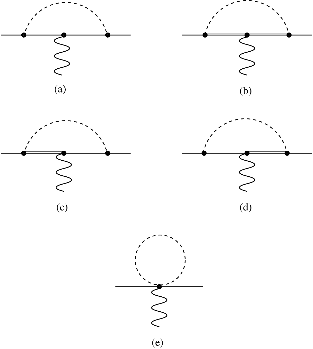
Having acquired the necessary physical motivation and mathematical tools, we are now ready to deal with baryon magnetic moments beyond tree level. The aim of this section is to provide a complete analysis of corrections to these observables at one-loop order in the framework of heavy baryon chiral perturbation theory in the large-$N_{c}$ limit. These corrections arise from the Feynman diagrams depicted in Figs. 1 and 2. The computation of the baryon operator structures involved in each diagram for finite $N_{c}$ (specifically for $N_{c}=3$) is presented in detail in this section. Computations at larger $N_{c}$ are less interesting physically and are by far more complicated to extrapolate to $N_{c}=3$ due to the participation of unphysical baryons as intermediate states in the loops [45]. We need, however, to emphasize that the approach we implement here has been simplified by working in the degeneracy limit $\Delta\equiv M_{T}-M_{B}\to 0$, where $M_{T}$ and $M_{B}$ are the SU(3) invariant masses of the decuplet and octet baryon multiplets, respectively. In the large-$N_{c}$ limit, although the mass of each baryon is order $\mathcal{O}(N_{c})$, $\Delta$ is order $\mathcal{O}(1/N_{c})$, so our assumption is a reasonable one. We now proceed to analyze each diagram separately.

References

• [1] P. Ha, Phys. Rev. D 58, 113003 (1998).
• [2] P. Ha and L. Durand, Phys. Rev. D 58, 093008 (1998).
• [3] J. Franklin, Phys. Rev. D 66, 033010 (2002).
• [4] H. Dahiya and M. Gupta, Phys. Rev. D 67, 114015 (2003).
• [5] B. Julia-Diaz and D. O. Riska, Nucl. Phys. A 739, 69 (2004).
• [6] K. Berger, R. F. Wagenbrunn and W. Plessas, Phys. Rev. D 70, 094027 (2004).
• [7] A. Faessler et. al, Phys. Rev. D 74, 074010 (2006).
• [8] J. Linde, T. Ohlsson and H. Snellman, Phys. Rev. D 57, 5916 (1998).
• [9] T. M. Aliev, A. Ozpineci and M. Savci, Phys. Rev. D 66, 016002 (2002) [Erratum-ibid. D 67, 039901 (2003)].
• [10] S. T. Hong, Phys. Rev. D 76, 094029 (2007).
• [11] L. Wang and F. X. Lee, Phys. Rev. D 78, 013003 (2008).
• [12] E. Jenkins and A. V. Manohar, Phys. Lett. B 335, 452 (1994).
• [13] J. Dai, R. F. Dashen, E. Jenkins and A. V. Manohar, Phys. Rev. D 53, 273 (1996).
• [14] E. Jenkins, X. d. Ji and A. V. Manohar, Phys. Rev. Lett. 89, 242001 (2002).
• [15] R. F. Lebed and D. R. Martin, Phys. Rev. D 70, 016008 (2004).
• [16] D. G. Caldi and H. Pagels, Phys. Rev. D 10, 3739 (1974).
• [17] J. Gasser, M. E. Sainio and A. Svarc, Nucl. Phys. B 307, 779 (1988).
• [18] A. Krause, Helv. Phys. Acta 63, 3 (1990).
• [19] E. Jenkins, M. E. Luke, A. V. Manohar and M. J. Savage, Phys. Lett. B 302, 482 (1993) [Erratum-ibid. B 388, 866 (1996)].
• [20] M. K. Banerjee and J. Milana, Phys. Rev. D 54, 5804 (1996).
• [21] U. G. Meissner and S. Steininger, Nucl. Phys. B 499, 349 (1997).
• [22] L. Durand and P. Ha, Phys. Rev. D 58, 013010 (1998).
• [23] S. J. Puglia and M. J. Ramsey-Musolf, Phys. Rev. D 62, 034010 (2000).
• [24] D. Arndt and B. C. Tiburzi, Phys. Rev. D 69, 014501 (2004).
• [25] L. S. Geng, J. M. Camalich, L. Alvarez-Ruso and M. J. V. Vacas, Phys. Rev. Lett. 101, 222002 (2008).
• [26] L. S. Geng, J. Martin Camalich and M. J. Vicente Vacas, Phys. Rev. D 80, 034027 (2009).
• [27] I. C. Cloet, D. B. Leinweber and A. W. Thomas, Phys. Lett. B 563, 157 (2003).
• [28] R. F. Dashen, E. Jenkins and A. V. Manohar, Phys. Rev. D 49, 4713 (1994) [Erratum-ibid. D 51, 2489 (1995)].
• [29] R. F. Dashen, E. Jenkins and A. V. Manohar, Phys. Rev. D 51, 3697 (1995).
• [30] E. Jenkins, Phys. Lett. B 315, 441 (1993).
• [31] E. Jenkins and R. F. Lebed, Phys. Rev. D 52, 282 (1995).
• [32] R. Flores-Mendieta, Phys. Rev. D 70, 114036 (2004).
• [33] R. Flores-Mendieta, E. Jenkins and A. V. Manohar, Phys. Rev. D 58, 094028 (1998).
• [34] E. Jenkins and A. V. Manohar, Phys. Lett. B 255, 558 (1991).
• [35] E. Jenkins and A. V. Manohar, Phys. Lett. B 259, 353 (1991).
• [36] V. Bernard, Prog. Part. Nucl. Phys. 60, 82 (2008).
• [37] R. Flores-Mendieta and C. P. Hofmann, Phys. Rev. D 74, 094001 (2006).
• [38] R. Flores-Mendieta, C. P. Hofmann, E. Jenkins and A. V. Manohar, Phys. Rev. D 62, 034001 (2000).
• [39] M. A. Luty and J. March-Russell, Nucl. Phys. B 426, 71 (1994).
• [40] M. A. Luty, J. March-Russell and M. J. White, Phys. Rev. D 51, 2332 (1995).
• [41] E. Jenkins, Phys. Rev. D 53, 2625 (1996).
• [42] C. Amsler et al. [Particle Data Group], Phys. Lett. B 667, 1 (2008).
• [43] S. R. Coleman and S. L. Glashow, Phys. Rev. Lett. 6, 423 (1961).
• [44] M. A. B. Beg, B. W. Lee and A. Pais, Phys. Rev. Lett. 13, 514 (1964).
• [45] Y. S. Oh and W. Weise, Eur. Phys. J. A 4, 363 (1999).
• [46] R. Flores-Mendieta, AIP Conf. Proc. 623, 232 (2002).
• [47] G. Lopez Castro and A. Mariano, Phys. Lett. B 517, 339 (2001).