Galaxy luminosities, stellar masses, sizes, velocity dispersions as a function of morphological type
Abstract
We provide fits to the distribution of galaxy luminosity, size, velocity dispersion and stellar mass as a function of concentration index and morphological type in the SDSS. (Our size estimate, a simple analog of the SDSS cmodel magnitude, is new: it is computed using a combination of seeing-corrected quantities in the SDSS database, and is in substantially better agreement with results from more detailed bulge/disk decompositions.) We also quantify how estimates of the fraction of ‘early’ or ‘late’ type galaxies depend on whether the samples were cut in color, concentration or light profile shape, and compare with similar estimates based on morphology. Our fits show that ellipticals account for about 20% of the -band luminosity density, , and 25% of the stellar mass density, ; including S0s and Sas increases these numbers to 33% and 40%, and 50% and 60%, respectively. The values of and , and the mean sizes, of E, E+S0 and E+S0+Sa samples are within 10% of those in the Hyde & Bernardi (2009), and samples, respectively. Summed over all galaxy types, we find Mpc-3 at . This is in good agreement with expectations based on integrating the star formation history. However, compared to most previous work, we find an excess of objects at large masses, up to a factor of at . The stellar mass density further increases at large masses if we assume different IMFs for elliptical and spiral galaxies, as suggested by some recent chemical evolution models, and results in a better agreement with the dynamical mass function.
We also show that the trend for ellipticity to decrease with luminosity is primarily because the E/S0 ratio increases at large . However, the most massive galaxies, , are less concentrated and not as round as expected if one extrapolates from lower , and they are not well-fit by pure deVaucouleur laws. This suggests formation histories with recent radial mergers. Finally, we show that the age-size relation is flat for ellipticals of fixed dynamical mass, but, at fixed , S0s and Sas with large sizes tend to be younger. Hence, samples selected on the basis of color or will yield different scalings. Explaining this difference between E and S0 formation is a new challenge for models of early-type galaxy formation.
Keywords:
galaxies: formation - galaxies: haloes - dark matter - large scale structure of the universe1 Introduction
Each galaxy has its own peculiarities. Nevertheless, even to the untrained eye, sufficiently well-resolved galaxies can be separated into three morphological types: disky spirals, bulgy ellipticals, and others which are neither. The morphological classification of galaxies is a field that is nearly one hundred years old, and sample sizes of a few thousand morphologically classified galaxies are now available (e.g. Fukugita et al. 2007; Lintott et al. 2008). However, such eyeball classifications are prohibitively expensive in the era of large scale sky surveys, which image upwards of a few million galaxies. Moreover, the morphological classification of even relatively low redshift objects from ground-based data is difficult. Thus, a number of groups have devised automated algorithms for discerning morphologies from such data (e.g. Ball et al. 2004 and references therein).
In parallel, it has been recognized that relatively simple criteria, using either crude measures of the light profile (e.g. Strateva et al. 2001), the colors (e.g. Baldry et al. 2004), or some combination of photometric and spectroscopic information (Bernardi et al. 2003; Bernardi & Hyde 2009) allow one to separate early-type galaxies from the rest. Because they are so simple, these tend to be more widely used. The main goal of this paper is to show how samples based on such crude cuts compare with those which are based on the eyeball morphological classifications of Fukugita et al. (2007). We do so by comparing the luminosity, stellar mass, size and velocity dispersion distributions for cuts based on photometric parameters with those based on morphology. These were chosen because the luminosity function is standard, although it is becoming increasingly common to compare models with rather than (e.g. Cole et al. 2001; Bell et al. 2003; Panter et al. 2007; Li & White 2009); the size distribution has also begun to receive considerable attention recently (Shankar et al. 2009b); and the distribution of velocity dispersions (Sheth et al. 2003) is useful, amongst other things, to reconstruct the mass distribution of super-massive black holes (e.g. Shankar et al. 2004; Tundo et al. 2007; Bernardi et al. 2007; Shankar, Weinberg & Miralda-Escudé 2009; Shankar et al. 2009a) and in studies of gravitational lensing (Mitchell et al. 2005).
Section 2 describes the dataset, the photometric and spectroscopic parameters derived from it, and the subsample defined by Fukugita et al. (2007). This section shows how we use quantities output from the SDSS database to define seeing-corrected half-light radii which closely approximate the result of bulge + disk decompositions. We describe our stellar mass estimator in this section as well; a detailed comparison of it with stellar mass estimates computed by three different groups is presented in Appendix A. The result of classifying objects into two classes, on the basis of color, concentration index, or morphology are compared in Section 3. Luminosity, stellar mass, size and velocity dispersion distributions, for the Fukugita et al. morphological types are presented in Section 4, where they are compared with those based on the other simpler selection cuts. This section includes a discussion of the functional form, a generalization of the Schechter function, which we use to fit our measurements. We find more objects with large stellar masses than in previous work (e.g. Cole et al. 2001; Bell et al. 2003; Panter et al. 2007; Li & White 2009); this is the subject of Section 5, where implications for the match with the integrated star formation rate, and the question of how the most massive galaxies have evolved since are discussed.
While we believe these distributions to be interesting in their own right, we also study a specific example in which correlations between quantities, rather than the distributions themselves, depend on morphology. This is the correlation between the half-light radius of a galaxy and the luminosity weighted age of its stellar population. Section 6 shows that the morphological dependence of this relation means it is sensitive to how the ‘early-type’ sample was selected, potentially resolving a discrepancy in the recent literature (Shankar & Bernardi 2009; van der Wel et al. 2009; Shankar et al. 2009c). A final section summarizes our results, many of which are provided in tabular form in Appendix B.
Except when stated otherwise, we assume a spatially flat background cosmology dominated by a cosmological constant, with parameters , and a Hubble constant at the present time of km s-1Mpc-1. When we assume a different value for , we write it as km s-1Mpc-1.
2 The SDSS dataset
2.1 The full sample
In what follows, we will study the luminosities, sizes, velocity dispersions and stellar masses of a magnitude limited sample of SDSS galaxies with in the band, selected from 4681 deg2 of sky. In this band, the absolute magnitude of the Sun is .
The SDSS provides a variety of measures of the light profile of a galaxy. Of these the Petrosian magnitudes and sizes are the most commonly used, because they do not depend on fits to models. However, for some of what is to follow, the Petrosian magnitude is not ideal, since it captures a type-dependent fraction of the total light of a galaxy. In addition, seeing compromises use of the Petrosian sizes for almost all the distant lower luminosity objects, leading to systematic biases (see Hyde & Bernardi 2009 for examples).
Before we discuss the alternatives, we note that there is one Petrosian based quantity which will play an important role in what follows. This is the concentration index , which is the ratio of the scale which contains 90% of the Petrosian light in the -band, to that which contains 50%. Early-type galaxies, which are more centrally concentrated, are expected to have larger values of , and two values are in common use: a more conservative (e.g. Nakamura et al. 2003; Shen et al. 2003) and a more cavalier (e.g. Strateva et al. 2001; Kauffmann et al. 2003; Bell et al. 2003). We show below that from the first approximately two-thirds of the sample comes from E+S0 types, whereas the second selects a mix in which E+S0+Sa’s account for about two-thirds of the objects.


The SDSS also outputs deV or exp magnitudes and sizes which result from fitting to a deVaucouleur or exponential profile, and fracDev, a quantity which takes values between 0 and 1, which is a measure of how well the deVaucouleur profile actually fit the profile (1 being an excellent fit). In addition, it outputs cmodel magnitudes; this is a very crude disk+bulge magnitude which has been seeing-corrected. Rather than resulting from the best-fitting linear combination of an exponential disk and a deVaucouleur bulge, the cmodel magnitude comes from separately fitting exponential and deVaucouleur profiles to the image, and then combining these fits by finding that linear combination of them which best-fits the image. Thus, if and are the magnitudes returned by fitting the two models, then
| (1) | |||||
Later in this paper, we will be interested in seeing-corrected half-light radii. We use the cmodel fits to define these sizes by finding that scale where
| (2) | |||||
where is the surface brightness associated with the two fits. Note that the SDSS actually performs a two dimensional fit to the image, and it outputs the half-light radius of the long axis of the image a, and the axis ratio b/a. The expression above assumes one dimensional profiles, so we use the half-light radius a of the exponential fit, and for the deVaucouleur fit. We describe some tests of these cmodel quantities shortly.
We would also like to study the velocity dispersions of these objects. One of the important differences between the SDSS-DR6 and previous releases is that the low velocity dispersions ( km s-1) were biased high; this has been corrected in the DR6 release (see DR6 documentation, or discussion in Bernardi 2007). The SDSS-DR6 only reports velocity dispersions if the in the spectrum in the restframe Å is larger than 10 or with the status flag equal to 4 (i.e. this tends to exclude galaxies with emission lines). To avoid introducing a bias from these cuts, we have also estimated velocity dispersions for all the remaining objects (see Hyde & Bernardi 2009 for more discussion). These velocity dispersions are based on spectra measured through a fiber of radius 1.5 arcsec; they are then corrected to , as is standard practice. (This is a small correction.) The velocity dispersion estimate for emission line galaxies can be compromised by rotation. In addition, the dispersion limit of the SDSS spectrograph is km s-1, so at small the estimated velocity dispersion may both noisy and biased. We will see later that this affects the velocity dispersion function. The size and velocity dispersion can be combined to estimate a dynamical mass; we do this by setting .
2.2 A morphologically selected subsample
Recently, Fukugita et al. (2007) have provided morphological classifications (Hubble type T) for a subset of 2253 SDSS galaxies brighter than in the band, selected from 230 deg2 of sky. Of these, 1866 have spectroscopic information. Since our goal is to compare these morphological selected subsamples with those selected based on relatively simple criteria (e.g. concentration index), we group galaxies classified with half-integer T into the smaller adjoining integer bin (except for the E class; see also Huang & Gu 2009 and Oohama et al. 2009). In the following, we set E (T = 0 and 0.5), S0 (T = 1), Sa (T = 1.5 and 2), Sb (T = 2.5 and 3), and Scd (T = 3.5, 4, 4.5, 5, and 5.5). This gives a fractional morphological mix of (E, S0, Sa, Sb, Scd) = (0.269, 0.235, 0.177, 0.19, 0.098). Note that this is the mix in a magnitude limited catalog – meaning that brighter galaxies (typically earlier-types) are over-represented.
2.3 cmodel magnitudes and sizes
As a check of our cmodel sizes, we have performed deVaucouleurs bulge + exponential disk fits to light profiles of a subset of the objects; see Hyde & Bernardi (2009) for a detailed description and tests of the fitting procedure. If we view these as the correct answer, then the top left panel of Figure 1 shows that the cmodel magnitudes are in good agreement with those from the full bulge+disk fit, except at fracDev and fracDev where cmodel is fainter by 0.05 mags (top left). This is precisely the regime where the agreement should have been best. As discussed shortly, the discrepancy arises mainly because the SDSS reductions suffer from sky subtraction problems (see, e.g., SDSS DR7 documentation), whereas our bulge-disk fits do not (see Hyde & Bernardi 2009 for details). Comparison with the top right panel shows that cmodel is a significant improvement on either the deV or the exp magnitudes alone.
| Sample | |||
| fracDev | |||
| & arcsec | 0.582 | 0.065 | |
| & arcsec | 0.249 | 0 | 0 |
| fracDev | |||
| & arcsec | 0.201 | 0.015 | |
| & arcsec | 0.182 | 0 | 0 |
| fracDev | |||
| & arcsec | 0.368 | 0.021 | |
| & arcsec | 0.231 | 0 | 0 |
| Sample | |||
| fracDev | 0 | ||
| fracDev | |||
| & arcsec | 0.147 | 0 | |
| & arcsec | 0 | 0 | 0 |
| fracDev | 0 | 0.001 |
The bottom panels show a similar comparison of the sizes. At intermediate values of fracDev, neither the pure deVaucouleur nor the pure exponential fits are a good description of the light profile, so the sizes are also biased (bottom right). However, at fracDev=1, where the deVaucouleurs model should be a good fit, the deV sizes returned by the SDSS are about 0.07 dex smaller than those from the bulge+disk decomposition. There is a similar discrepancy of about 0.05 dex with the SDSS Exponential sizes at fracDev=0. We argue below that these offsets are related to those in the magnitudes, and are primarily due to sky subtraction problems.
The filled circles in the bottom left panel show that our cmodel sizes (from equation 2) are in substantially better agreement with those from the bulge+disk decomposition over the entire range of fracDev, with a typical scatter of about 0.05 dex (inner set of dashed lines). For comparison, the triangles show the result of picking either the deVaucouleur or exponential size, based on which of these magnitudes were closer to the cmodel magnitude (this is essentially the scale that the SDSS uses to compute model colors). Note that while this too removes most of the bias (except at small fracDev), it is a substantially noisier estimate of the true size (outer set of dashed lines). This suggests that our cmodel sizes, which are seeing corrected, represent a significant improvement on what has been used in the past.
The SDSS reductions are known to suffer from sky subtraction problems which are most dramatic for large objects or objects in crowded fields (see DR7 documentation). The top panels in Figure 2 show this explicitly: while there is little effect at small size, the SDSS underestimates the brightnesses and sizes when the half-light radius is larger than about 5 arcsec. Note that this is actually a small fraction of the objects: 6% of the objects have sdss-cmodel sizes larger than 5 arcsec; 13% are larger than 4 arcsec. Whereas previous work has concentrated on mean trends for the full sample, Figure 2 shows that, in fact, the difference depends on the type of light profile – galaxies with fracDev (i.e. close to deVaucouleur profiles) are more sensitive to sky-subtraction problems than later-type galaxies. Some of this is due to the fact that such galaxies tend to populate more crowded fields.
To correct for this effect, we have fit low order polynomials to the trends; the solid curves in the top panels of Figure 2 show these fits. Except for the sample with fracDev , we use these fits to define our final corrected cmodel sizes by:
| (3) | |||||
and
| (4) | |||||
where the coefficients , , , , and are reported in Table 1.
For objects with fracDev , the trends we see are similar to those shown in Fig. 5 of Hyde & Bernardi (2009), which were based on a (larger) sample of about early-type galaxies. The thick solid (magenta) line in the top panels of Figure 2 show the Hyde-Bernardi trends, with a small offset to account for the fact that they did not integrate the fitted profiles to infinity (because the SDSS, to which they were comparing, does not), whereas we do. The thick solid curve differs from the thin one at sizes larger than about 5 arcsec. Since the thick curve is based on a larger sample, we use it to define our final corrected cmodel sizes. The corrections are again described by equations (3) and (4), with coefficients that are reported in Table 1.
The bottom panels of Figure 2 show that these corrected quantities agree quite well with those from the full bulge+disk fit, even at small and large fracDev.
2.4 Stellar Masses
Stellar masses are typically obtained by estimating (in solar units), and then multiplying by the restframe (which is not evolution corrected). In the following we compare three different estimates of . All these estimates depend on the assumed IMF: Table 2 shows how we transform between different IMFs.
The first comes from Bell et al. (2003), who report that, at , , where the zero-point depends on the IMF (see their Appendix 2 and Table 7). Their standard diet-Salpeter IMF has , which they state has 70% smaller at a given color than a Salpeter IMF. In turn, a Salpeter IMF has 0.25 dex more at a given color than the Chabrier (2003) IMF used by the other two groups whose mass estimates we use (see Table 2 for conversion of different IMFs). Therefore, we set , making
| (5) |
We then obtain by multiplying by the SDSS band luminosity. When comparing with previous work, we usually use Petrosian magnitudes, although our final results are based on the cmodel magnitudes which we believe are superior.
Note that this expression requires luminosities and colors that have been - and evolution-corrected to (E. Bell, private communication). Unfortunately, these corrections are not available on an object-by-object basis. Bell et al. (2003) report that the absolute magnitudes brighten as and color becomes bluer as . Although these estimates differ slightly from independent measurements of evolution by Bernardi et al. (2003) and Blanton et al. (2003), and more significantly from more recent determinations (Roche et al. 2009a), we use them, because they are the ones from which equation (5) was derived. Thus, in terms of restframe quantities,
| (6) |
If we use the restframe color and luminosity instead, then
| (7) |
| IMF | Offset [dex] | Refecence |
|---|---|---|
| Kennicut | 0.30 | Kennicut (1983) |
| Scalo | 0.25 | Scalo (1986) |
| diet-Salpeter | 0.15 | Bell & de Jong (2001) |
| pseudo-Kroupa | 0.20 | Kroupa (2001) |
| Kroupa | 0.30 | Kroupa (2002) |
| Chabrier | 0.25 | Chabrier (2003) |
| Baldry & Glazbrook | 0.305 | Baldry & Glazbrook (2003) |
These two estimates of will differ because there is scatter in the color plane. Unfortunately, Bell et al. do not provide a prescription which combines different colors. Although we could perform a straight average of these two estimates, this is less than ideal because the value of at fixed may provide additional information about . In practice, we will use the estimate as our standard, and to illustrate and quantify intrinsic uncertainties with the current approach.
The second estimate of is from Gallazzi et al. (2005). This is based on a likelihood analysis of the spectra, assumes the Chabrier (2003) IMF, and returns . The stellar mass is then computed using SDSS petrosian -band restframe magnitudes (i.e., they were -corrected, but no evolution correction was applied). In this respect, they differ in philosophy from , in that the estimate is not corrected to . In practice, since we are mainly interested in small lookback times from , for which the expected mass loss to the IGM is almost negligible, this almost certainly makes little difference for the most massive galaxies. These estimates are only available for of the objects in our sample (). The objects for which Gallazzi et al. do not provide stellar mass estimates are lower luminosity, typically lower mass objects; we show this explicitly in Figure 20.
A final estimate of comes from Blanton & Roweis (2007), and is based on fitting the observed colors in all the SDSS bands to templates of a variety of star formation histories and metallicities, assuming the Chabrier (2003) IMF. In the following we use the Blanton & Roweis stellar masses computed by applying the SDSS petrosian and model (restframe) -magnitudes to these mass-to-light estimates: and . Blanton & Roweis also provide mass estimates from a template which is designed to match luminous red galaxies; we call these . Note that in this case is converted to using (restframe) model magnitudes only, since the Petrosian magnitude is well-known to underestimate (by about 0.1 mags) the magnitudes of LRG-like objects (Blanton et al. 2001, DR7 documentation). To appreciate how different the LRG template is from the others, note that it allows ages of upto 10 Gyrs, whereas that for the others, the age is more like 7 Gyrs.
A detailed comparison of the different mass estimates is presented in Appendix A. This shows that to use the Blanton & Roweis (2007) masses, one must devise an algorithm for choosing between and . In principle, some of the results to follow allow one to do this, but exploring this further is beyond the scope of the present paper. On the other hand, to use the Gallazzi et al. (2005) estimates, one must be wary of aperture effects. Finally, stellar masses based on the corrected color show stronger systematics than do the based estimates of . Therefore, in what follows, our prefered mass estimate will be that based on corrected cmodel magnitudes and colors (i.e., equation 6 with restframe and evolution corrected magnitudes and colors). Note that we believe the cmodel magnitudes to be far superior to the Petrosian ones. Of course, when we compare our results with previous work which used Petrosian magnitudes (Section 5), we do so too.


3 Morphology and sample selection
This section compares a number of ways in which early-type samples have been defined in the recent literature, with the morphological classifications of Fukugita et al., and discusses what this implies for the ‘red’ fraction. When we show luminosities, they have been corrected for evolution by assuming that the magnitudes brighten with redshift as .
3.1 Simple measures of the light profile
Concentration index, axis ratio, and fracdev have all been used as proxies for selecting red, massive, early-type galaxies. So it is interesting to see how these quantities correlate with morphological type.
The bottom right panel of Figure 3 shows the distribution of all objects in the Fukugita et al. sample in the space of concentration versus luminosity. The two horizontal lines show and , the two most popular choices for selecting early-type samples. The symbols with error bars show the mean concentration index at each if the sample is selected following Hyde & Bernardi (2009): i.e. fracDev in - and -, and -band . To this we add the condition log, which is essentially a cut on color gradient (Roche et al. 2009b). This removes a small fraction (%) of late-type galaxies which survive the other cuts. Dashed curves show the scatter around the -luminosity relation in the Hyde & Bernardi sample.
The other panels show the result of separating out the various morphological types. Whereas Es and S0s occupy approximately the same region in this space, most Es (93%) have , whereas the distribution of for S0s is somewhat less peaked. (Here, the percentages we quote are per morphological type, in the Fukugita et. al. sample – meaning a sample that is magnitude-limited to , with no weighting applied.) Samples restricted to have a substantial contribution from both Sas ( of which satisfy this cut) and S0s (for which this fraction is ), and this remains true even if ( of Sas and of S0s). Thus, it is difficult to select a sample of Es on the basis of concentration index alone. On the other hand, the larger mean concentration of the Hyde & Bernardi selection cuts suggest that they produce a sample that is dominated by ellipticals/S0s, and less contaminated by Sas (see Section 3.5 and Table 3 below). Figure 4 shows that replacing luminosity with stellar mass leads to similar conclusions.
Before moving on, notice that although the mean concentration increases with luminosity and stellar mass in the Hyde & Bernardi sample, this is no longer the case at the highest or : we will have more to say about this shortly.
Figures 5 and 6 show a similar analysis of the axis ratio . The different symbols with error bars (same in all panels) show samples selected to have , , and following Hyde & Bernardi. At or so, the mean in the first two cases increases with luminosity upto or so; it decreases for the brightest objects. At low , the sample with has smaller values of on average, though the scatter around the mean is large. Morevoer, while there are essentially no Es with about of S0s have . On the other hand, a little less than half the Sa’s and many Scd’s also have (because they are face on). Evidently, just as alone is not a good way to select a pure sample of ellipticals, selecting on alone is not good either.
The filled red circles (with error bars) in the top left panel show that, for Es, independent of , except at the highest luminosities where decreases. This independence of differs markedly from that in either of the samples, but is reproduced by the Hyde & Bernardi sample, for which except at where it decreases. The difference of about 0.05 in arises because the Hyde & Bernardi sample includes some S0s (we quantify this in Table 3 below), for which (filled red circles in top right panel). This leads to an important point. While it has long been known that tends to increase with luminosity, even in ‘early-type’ samples, our Figure 5 shows that this increase is driven by the changing morphological mix – the change from S0s to Es – at . Whether this is due to environmental or pure secular evolution effects is an open question.
On the other hand, there is a plausible, environmentally driven model for the decrease in at the highest . This decrease has been expected for some time (see González-García & van Albada 2005; Boylan-Kolchin et al. 2006 and references therein) – it was first found by Bernardi et al. (2008). This is thought to indicate an increasing incidence of radial mergers, since these would tend to result in more prolate objects. The decrease in concentrations at these high luminosities (Figure 3) is consistent with this picture, as is the fact that most of these high luminosity objects are found in clusters. All of the preceding discussion remains true if one replaces luminosity with stellar mass.


Before concluding this section, we note that we have also considered the quantity fracdev which plays an important role in the selection cuts used by Hyde & Bernardi (2009). The vast majority of ellipticals (85%) have fracdev=1, with only a percent or so having fracdev. The distribution of fracdev has a broader peak for S0s, but they otherwise cover the same range as Es: only 37% have fracdev. However, 70% of Sas have fracdev, whereas for Scs’s, only 10% have fracdev. (Note that the above percentages were computed in the magnitude limited catalog, i.e. were not weighted by .)
3.2 Colors
In addition to simple measures based on the light profile, or more commonly, as an alternative to such methods, color is sometimes used as a way to selecting early types. This is typically done by noting that the color-magnitude distribution is bimodal (e.g. Baldry et al. 2005), and then adopting a crude approximation to this bimodality (e.g. Zehavi et al. 2005; Blanton & Berlind 2007; Skibba & Sheth 2009). Figure 7 shows this bimodal distribution in the Fukugita et al. sample (Figure 8 shows the corresponding color- relation). The dotted green line in Figure 7, shows
| (8) |
It runs approximately parallel to the ‘red’ sequence, and is similar to that obtained by subtracting mags from equation (4) in Skibba & Sheth (2009); it is shallower than equation (7) in Skibba & Sheth (2009) or equation (1) of Young et al. (2009) (note that we -correct to and we use ). ‘Red’ galaxies are those which lie above this line; ‘blue’ lie below it.


However, note that many late types (Sb and later) lie above this line – these tend to be edge-on disks. In addition, some Es lie below it. (See Huang & Gu 2009 for a more detailed analysis of such objects, which show either a star forming, AGN or post-starburst spectrum.) We intend to present a more detailed study of the morphological dependence of the color-magnitude, stellar mass and velocity dispersion relations in a future paper (Bernardi et al. 2009, in preparation). For our purposes here, we simply note that Figures 7 and 8 illustrate that cuts in color are not a good way to select early-type galaxies.
3.3 Ages
Later in this paper, we will also study correlations between stellar age and galaxy mass, size and morphology. The age estimates we use, from Gallazzi et al. (2005), are based on a detailed analysis of spectral features. Since this is the same analysis that provided , errors in age and stellar mass are correlated (see Bernardi 2009 for a detailed discussion): erroneously large will tend to have erroneously large age as well.
Figure 9 shows the age- correlation for the objects in the Fukugita et al. sample for which age estimates are available. This shows that, for any given morphological type, massive galaxies tend to be older (this correlation is not due to correlated errors). However, as expected, the later types tend to be substantially younger: Whereas two-thirds of the Es in this sample are older than 8 Gyrs, only half of S0s, one-quarter of Sas, and fewer than 10 % of the later types (Sb, Sc, etc.) are this old. The bottom right panel suggests that the age- distribution separates into two populations – one which is younger than about 7 Gyrs and another which is older. However, this is not simply correlated with morphological type: the top panels shows that this bimodality is also present in the E and S0s samples.
To study this further Figure 10 shows the age- distribution in a random subsample of the galaxies selected following Hyde & Bernardi (2009) from the full SDSS catalog. Note that although 90% of the objects are older than 6 Gyrs, this selection clearly includes a population of younger objects. This population of ‘rejuvenated’ early-type galaxies has been the subject of some recent interest (e.g. Huang & Gu 2009; Thomas et al. 2010). Cyan filled circles show that the median age increases with stellar mass and dashed lines show the range around the median. Green diamonds and magenta squares show the median age at fixed stellar mass for objects with and , respectively. At large , both these samples produce similar age- relations to the Hyde-Bernardi sample; at smaller , allowing smaller includes younger galaxies. These median relations are superimposed on the panels of Figure 9.
3.4 The red and blue fractions
There is considerable interest in the ‘build-up’ of the red sequence, and the possibility that some of the objects in the blue cloud were ‘transformed’ into redder objects. We now compare estimates of the red or blue fraction that are based on color and concentration, with ones based on morphology. In particular, we show how these fractions vary as a function of , , and .
All the results which follow are based on samples which are Petrosian magnitude limited, so in all the statistics we present, each object is weighted by , the inverse of the maximum volume to which it could have been seen. This magnitude limit is fainter for the full sample () than it is for the Fukugita et al. subsample (), and note that depends on our model for how the luminosities evolve (absolute magnitudes brighten as ).
The panels on the left of Figure 11 show how the mix of objects changes as a function of luminosity, stellar mass, and velocity dispersion, for the crude but popular hard cuts in concentration and color (as described in the the previous sections).
Figure 11 shows that the fraction of objects which satisfies the criteria used by Hyde & Bernardi (2009) increases with increasing , and , except at the largest values (about which, more later). Requiring instead results in approximately 5% to 10% more objects (compared to the Hyde & Bernardi cuts) at each or ; although, in the case of km s-1, this cut allows about 20% more objects. Relaxing the cut to allows an additional 15%, with slightly more at intermediate and .
Selecting objects redder than a luminosity dependent threshold (equation 8) which runs parallel to the ‘red’ sequence allows even more objects into the sample, but combining the color cut with one on reduces the sample to one which resembles rather well. The cut in is easy to understand, since edge-on discs will lie redward of the color cut even though they are not early-types – the additional cut on is an easy (but rarely used!) way to remove them.
It is interesting to compare these panels with their counterparts on the right of Figure 11, in which later and later morphological types are added to the Fukugita et al. subsample which initially only contains Es. This suggests that the Hyde & Bernardi selection will be dominated by E, will be dominated by E+S0s, and will be dominated by E+S0+Sas. We quantify this in the next subsection. Figure 12 shows a similar comparison with the blue fraction. Note that the contamination of the red fraction by edge-on discs is a large effect: 60% of the objects at are classified as being red, when E+S0+Sas sum to only 40%. Figure 13 shows this more directly: the reddest objects at intermediate luminosities are late-, not early-type galaxies.
Before concluding this section, we note that both concentration cuts greatly underpredict the red fraction of the most luminous or massive objects, as does the application of a cut to the straight color selection or the Hyde & Bernardi selection. The most luminous or massive elliptical galaxies in the Fukugita et al. sample show the same behavior. I.e., the most massive objects are less concentrated for their luminosities than one might have expected by extrapolation from lower luminosities and their light profile is not well represented by a pure deVaucoleur law. This is consistent with results in the previous section where, at the highest luminosities, tends to decrease with luminosity (Figure 5). These trends suggest an increasing incidence of recent radial mergers for the most luminous and massive galaxies.
3.5 Distribution of morphological types in differently selected samples
| Type | HB09 | ||
|---|---|---|---|
| E | 0.69 (0.73) | 0.38 (0.51) | 0.26 (0.43) |
| S0 | 0.23 (0.20) | 0.22 (0.23) | 0.20 (0.22) |
| Sa | 0.07 (0.06) | 0.25 (0.17) | 0.30 (0.20) |
| Sb | 0.01 (0.01) | 0.12 (0.07) | 0.19 (0.12) |
| Scd | - | 0.03 (0.02) | 0.05 (0.03) |
Much of the previous analysis suggests that the Hyde & Bernardi selection will produce a sample that is dominated by Es, will include more S0s and Sas, and will include Sas and later types. Table 3 shows the distribution of types in subsamples selected from the Fukugita et al. (2007) catalog to have , and following Hyde & Bernardi (2009). Of the 1596 objects in the magnitude limited catalog, 1009, 802 and 470 satisfy these cuts. The Table shows that, in samples where , 54% of the objects are Sa or later. This fraction falls to 40% for and to less than 10% for the Hyde-Bernardi cuts (these numbers are obtained after weighting by , so they do not depend on the selection effect associated with the apparent magnitude limit of the catalog).
These numbers indicate that Es comprise at least two-thirds of the Hyde-Bernardi sample, but in a sample where , to reach this fraction one must include S0s, and if , then reaching this fraction requires adding Sas as well. Stated differently, E’s comprise more than two-thirds of a Hyde-Bernardi sample, but about one-third of a sample with and one quarter of a sample with . If we weight each object by its stellar mass, then (E+S0)s account for (72+21)% of the total stellar mass in a Hyde & Bernardi sample, (47+23)% in a sample with , and (39+23)% if . These differences will be important in Section 6.
4 Distributions for samples cut by morphology or concentration
We now show how the luminosity, stellar mass, size and velocity dispersion distributions – , , and – depend on how the sample was defined. We use the same popular cuts in concentration as in the previous Sections, and , which we suggested might be similar to selecting early-type samples which, in addition to Es, include S0s + Sas, and S0s + Sas + Sbs, respectively. We then make similar measurements in the Fukugita et al. subsample, to see if this correspondence is indeed good.
In this Section, we use cmodel rather than Petrosian quantities, for the reasons stated earlier. The only place where we continue to use a Petrosian-based quantity is when we define subsamples based on concentration, since is the ratio of two Petrosian-based sizes, or for comparison with results from previous work.
The results which follow are based on samples which are Petrosian magnitude limited, so in all the statistics we present, each object is weighted by , the inverse of the maximum volume to which it could have been seen. In addition to depending on the magnitude limit ( for the full sample, and for the Fukugita subsample), the weight also depends on our model for how the luminosities have evolved. A common test of the accuracy of the evolution model is to see how , the ratio of the volume to which an object was seen to that which it could have been seen, averaged over all objects, differs from 0.5. In the full sample, it is for our assumption that the absolute magnitudes evolve as ; had we used (Blanton et al. 2003), it would have been . On the other hand, if we had ignored evolution entirely, it would have been 0.527.
In addition, SDSS fiber collisions mean that spectra were not taken for about 7% of the objects which satisfy . We account for this by dividing our weighted counts by a factor of 0.93. This ignores the fact that fiber collisions matter more in crowded fields (such as clusters); so in principle, this correction factor has some scatter, which may depend on morphological type. We show below that, when we ignore this scatter, then our analysis of the full sample produces results that are in good agreement with those of Blanton et al. (2003), who account for the fact that this factor varies spatially. This suggests that the spatial dependence is small, so, in what follows, we ignore the fact that it (almost certainly) depends on morphological type.
4.1 Parametric form for the intrinsic distribution
We will summarize the shapes of the distributions we find by using the functional form
| (9) |
This is the form used by Sheth et al. (2003) to fit the distribution of velocity dispersions; it is a generalization of the Schechter function commonly fit to the luminosity function (which has , a slightly different definition of ). We have found that the increased flexibility which allows is necessary for most of the distributions which follow. This is not unexpected: at fixed luminosity, most of the observables we study below scatter around a mean value which scales as a power-law in luminosity (e.g. Bernardi et al. 2003; Hyde & Bernardi 2009). Because this mean does not scale linearly with , and because the scatter around the mean can be significant, then if is well-fit by a Schechter function, it makes little physical or statistical sense to fit the other observables with a Schechter function as well.
4.2 Effect of measurement errors
In practice, we will also be interested in the effect of measurement errors on the shape of the distribution. If the errors are Lognormal (Gaussian in ) with a small dispersion, then the observed distribution is related to the intrinsic one by
| (10) | |||||
| (11) |
The peak of occurs at , where . Since and are usually positive, errors typically act to decrease the height of the peak. Since the net effect of errors is to broaden the distribution, hence extending the tails, errors also tend to decrease . The expression above shows that, in the tail, errors matter more when is large.
Fitting to equation (10) rather than to equation (9) is a crude but effective way to estimate the intrinsic shape (i.e., to remove the effect of measurement errors on the fitted parameters), provided the measurement errors are small. The rms errors on are indeed small: , and so it is the results of these fits which we report in what follows. However, to illustrate which distributions are most affected by measurement error, we also show results from fitting to equation (9); in most cases, the differences between the returned parameters are small, except when .
In practice, the fitting was done by minimizing
| (12) |
where was of the weighted count in the th logarithmically spaced bin (and recall that, because of fiber collisions, the weight is actually ).


4.3 Covariances between fitted parameters
When fitting to equation (9), a reasonable understanding of the covariance between the fitted parameters can be got by asking that all parameter combinations give the same mean density (Sheth et al. 2003):
| (13) |
In practice, is determined essentially independently of the other parameters, so it is the other three parameters which are covariant. Hence, it is convenient to define
| (14) |
If is fixed to unity, then this becomes . But if is not fixed, then a further constraint equation can be got by asking that all fits return the same peak position or height. For distributions with broad peaks, it may be better to instead require that the second central moment,
| (15) |
be well reproduced. Thus, the covariance between and is given by requiring that equal the measured value for this ratio. The changes to these correlations are sufficiently small if we instead fit to equation (10), so we have not presented the algebra here.
4.4 Distributions for samples cut by concentration
Figure 14 shows and in the full sample (top curve in top panel), when one removes objects with (second from top), objects with (third from top), and when one selects early-types on the basis of a number of other criteria (bottom, following Hyde & Bernardi 2009). For comparison, the dotted curves show the measurement in the full sample when Petrosian quantities are used (i.e. from Figures 19 and 20).
The solid curves show the result of fitting to equation (9), and the dashed curves (almost indistinguishable from the solid ones, except at the most massive end) result from fitting to equation (10) instead, so as to remove the effects of measurement error on our estimate of the shape of the intrinsic distribution. To reduce the dynamic range, bottom panels show each set of curves divided by the associated solid curve (i.e., by the fit to the observed sample). The dotted lines in these bottom panels show that Petrosian based counts lie well below those based on cmodel quantities at or . The dashed lines in the bottom right panel show that the intrinsic distribution has been noticably broadened by errors above .
Figure 15 shows a similar analysis of and . For we also compare our results with those of Sheth et al. (2003). The Sheth et al. analysis was based on a sample selected by Bernardi et al. (2003), which was more like at large masses, but because of cuts on emission lines and S/N in the spectra, had few low mass objects. Indeed, at large , our measured is similar to theirs.
Tables 6–9 report the parameters of the fits (to equations 9 and 10) shown in Figures 14 and 15. It is worth noting that, for a given sample, the fits return essentially the same value of in all the tables, even though this was not explicitly required. And note that and are the distributions that are most sensitive to errors; the former because the errors are large, and the latter because is large.
4.5 Comparison with morphological selection
Figures 16 and 17 show , , and for the Fukugita et al. sample as one adds more and more morphological types. The smooth curves (same in each panel) show the fits to the samples shown in Figures 14 and 15. In the top panels of Figure 16 only, we also show the result of removing objects with before making the measurements. This allows a direct comparison with one of the curves from the previous Figure. Notice that this gives results which are very similar to those from the larger (fainter, deeper) full sample; the different magnitude limits do not matter very much.
The results of fitting equation (10) to the Fukugita subsamples are provided in Tables 6–9, which also show the associated luminosity and stellar mass densities, and the mean sizes. Ellipticals account for about 19% of the -band cmodel luminosity density and 25% of the stellar mass density; including S0s increases these numbers to 33% and 41%, and adding Sas brings the contributions to 50% and 60% respectively.
Note that the number, luminosity and stellar mass densities of Es – about Mpc-3, Mpc-3 and Mpc-3 respectively – are very similar to those of the early-type sample selected following Hyde & Bernardi (2009), as is the mean half-light radius of 3.2 kpc. Some of this match is fortuitous – we showed before that E’s account for about 70% of this sample, not 100%. However, this lack of purity is balanced by the fact that Hyde & Bernardi select about 75% of the Es, not 100%: the purity and completeness effects approximately cancel. Similarly, although requiring produces counts which are similar to those of E+S0s, about 40% of the sample is made of Sas and later types, but the purity again approximately cancels the incompleteness. Finally, the counts when are similar to those in the E+S0+Sa sample, although 25% of the objects are of later type.
5 The stellar mass function in the full sample
Our stellar mass function has considerably more objects at large than reported in previous work. Before we quantify this, we show the results of a variety of tests we performed to check that the discrepancy with the literature is real. This is important, since the high mass end has been the subject of much recent attention (e.g., in the context of the build-up of the red sequence).
5.1 Consistency checks
We first checked that we were able to reproduce previous results for the luminosity function. These have typically used Petrosian rather than cmodel magnitudes, and different conventions. The top panel in Figure 18 shows the result of estimating the luminosity function using Petrosian magnitudes (using the method and code as in the previous sections) and the curve show the Schechter function fits reported by Blanton et al. (2003). This agreement shows that our algorithms correctly transform between different conventions, and between different definitions of -corrections. It also shows that varying the evolution correction between the value reported by Blanton et al. () and that from Bell et al. (), which we use when estimating stellar masses, makes little difference.


The bottom panel shows the Schechter function fit reported by Bell et al. (2003); there is good agreement. However, note that here we have not shifted the Petrosian magnitudes brightwards by 0.1 mags for galaxies with (Bell et al. did this to account crudely for the fact that Petrosian magnitudes underestimate the luminosity of early-types). At faint luminosities, the measurements oscillate around the fits, suggesting that fits to the sum of two Schechter functions will provide better agreement, but we do not pursue this further here. At the bright end, we find slightly more objects than either of the Bell et al. (top) or Blanton et al. (bottom) fits, but a glance at Fig. 5 in Blanton et al. shows that the fit they report slightly underestimates the counts in the high luminosity tail.
In contrast to the good agreement for the luminosity function, our estimates of the stellar mass function (Figure 20) show a significant excess relative to previous work at . (Note that, to compare with previous work, we convert from to by using the Petrosian magnitude. However, we do not shift the Petrosian magnitudes brightwards by 0.1 mags for galaxies with – a shift that was made by Bell et al. (2003). If we had done so the excess would be even larger). To ensure that the discrepancy with previous fits is not caused by outliers, we removed galaxies with or which differ by more than 0.3 dex from the linear fit (solid line in Figure 21), in luminosity or . Except for the based , where we show results before and after removal of these outliers, all the other measurements shown in Figure 20 are from the sample in which these outliers have been removed. Note that while removing outliers makes the plot slightly cleaner (see Figure 20), the discrepancy at high remains.
The discrepancy is most severe if we use stellar masses from Gallazzi et al. (2005). (Note that they do not provide stellar mass estimates for fainter, typically lower mass objects.) The discrepancy is slightly smaller if we use equation (6) to translate color into (for which both and are evolution corrected; if we had used restframe quantities without correcting for evolution the discrepancy would be even worse). Using instead (equation 7) yields results which are more similar to the original Bell et al. (2003) fit. And finally, based on of Blanton & Roweis (2007) has the lowest abundances of all.


The dotted line shows that our measurement of the distribution of is well-fit (except for a small offset) by the formula reported by Li & White (2009), which was based on their own estimate of from Blanton & Roweis . The fact that we find good agreement with their fit suggests that our algorithm for estimating from a given list of values is accurate.
The dashed-dot-dot green line shows the fit reported by Panter et al. (2007) who computed stellar masses for a sample of SDSS galaxies based on the analysis of the spectral energy distribution of the SDSS spectra. While this fit lies slightly below our data at high , the discrepancy is smaller than it is for most of the other fits we show.
We argued previously that aperture effects may have inflated the Gallazzi et al. masses slightly. As a check, we recomputed masses from the color using equation (6), but now, using the Fiber color output by the SDSS pipeline. In contrast to the model color, which measures the light on a scale which is proportional to the half-light radius, this measures the light in an aperture which has the same size as the SDSS fiber. The spectro-photometry of the survey is sufficiently accurate that this is a meaningful comparison (e.g. Roche et al. 2009a). Note that this gives abundances which are larger than those based on the model colors. Moreover, they are almost indistinguishable from those of .
The cyan solid curve shows the result of fitting equation (9) to our measurements of based on color (we do not show fits to equation 10, because none of the other fits in the literature account for errors in the stellar mass estimate) when . The best-fit parameters are reported in Table 4. The Table also reports the fit to the full sample (i.e. ). (These differ from those reported in the previous section, because here they are based on Petrosian rather than cmodel magnitudes.) The Figures show the results for and because this is the regime of most interest here.
Our estimates depart from the Bell et al. fit at densities of order Mpc-3. However, their analysis was based on only 412 deg2 of sky, for which the expected number of objects on the mass scale where we begin to see a discrepancy () is of order tens. This, we suspect, is the origin of the discrepancy between our results and theirs – we are extrapolating their fit beyond its regime of validity.
Bell et al. (2003) did not account for errors, so the most straightforward way to quantify the increase we find is to compare our measured counts with their fit. If we do this for our Petrosian-based counts, then the stellar mass density in objects more massive than is percent larger than one would infer from the Bell et al. fit. However, Bell et al. attempted to account for the fact that Petrosian magnitudes underestimate the total light by shifting galaxies with brightwards by 0.1 mags. Since we have not performed such a shift, the appropriate comparison with their fit is really to use our measured cmodel based counts, so the difference between our counts and Bell et al. are actually larger. We do this in the next section.
If we compare our estimate of the stellar mass density in objects more massive than with those from the Li & White (2009) fit, then our values are percent larger.
5.2 Towards greater accuracy at large
It is well known that the cmodel luminosities are more reliable at the large masses where the discrepancy in is largest. Therefore, Figure 22 compares various estimates of based on cmodel magnitudes. In this case, the estimates based on of Blanton & Roweis (2007) produce the lowest abundances, (but note they are larger than those based on in Figure 20), whereas those based on are substantially larger, as one might expect (c.f. Figure 32). The abundances are also in good agreement (slightly smaller) with those based on color (equation 6, with cmodel magnitudes), except at smaller masses. (Although it is not apparent because of how we have chosen to plot our measurements, above , the abundances based on and are in good agreement.)
We argued previously that we believe the masses are more reliable than those based on . Therefore, we only show fits to the distribution of derived masses: solid and dashed curves show fits to equation (9) and (10) respectively (the latter account for broadening of the distribution due to errors in the determination of ). Both result in larger abundances than the observed abundances based on Petrosian quantities – here represented by the fit shown in the previous figure – although the intrinsic distribution we determine for the cmodel based masses is similar to the observed distribution of Petrosian-based masses.
If we sum up the observed counts to estimate the stellar mass density ( from equation 6) in objects more massive than , then the result is percent larger than that one infers from the Bell et al. (2003) fit. Using our fit to the observed distribution (values between round brackets in Table 7, for ) gives similar results: stellar mass densities percent larger than those from the Bell et al. (2003) fit. In practice, however, the Bell et al. fit tends to be used as though it were the intrinsic quantity, rather than the one that has been broadened by measurement error. Our fit to the intrinsic distribution, based on cmodel magnitudes (from Table 7, for ) gives stellar mass densities in objects more massive than of Mpc-3. This corresponds to an extra percent more than from the Bell et al. fit.


| Sample | |||||
|---|---|---|---|---|---|
| All | () | () | () | () | |
| All | () | () | () | () | |
| All | () | () | () | () | |
| All | () | () | () | () |


Another way to express this difference is in terms of the mass scale at which the integrated comoving number density of objects is Mpc-3. For our fits to the intrinsic cmodel based counts, this scale is ( for the observed fit), whereas for Bell et al. (2003) it is . For Mpc-3, these scales are ( for the observed fit) and , respectively. Figure 23 illustrates these differences graphically. Note that the stellar masses used by Panter et al. and Li & White were obtained using Petrosian magnitudes. To account for the difference between Petrosian and model luminosities one could add dex to their values of (strictly speaking, to those objects with ) – we have not applied such a shift.
5.3 On major dry mergers at high masses
The increase in counts at high masses matters greatly in studies which seek to constrain the growth histories of massive galaxies by comparing with counts at . Figure 24 shows a closer-up view of the top panel of Figure 23. The plot is in the same format as Figure 3 in Bezanson et al. (2009). We have added a (solid magenta) curve showing the cumulative counts at from Marchesini et al. (2009), shifted to our Chabrier IMF by subtracting 0.05 dex from their values. The dashed curve below it shows the same counts shifted downwards by a factor of two, to reflect the fact that only perhaps half of the galaxies at are quiescent.

| Sample | Mpc-3 | Mpc-3 | |||
|---|---|---|---|---|---|
| IMF | () | () | () | () | |
| IMF | () | () | () | () | |
| () | () | () | () | ||
| () | () | () | () |
Bezanson et al. (2009) argue that models in which the high redshift objects change their sizes but not their masses by the present time (e.g. Fan et al. 2008) lie well below the counts. Because this results in an order of magnitude fewer counts than observed at , such models, while viable, do not represent the primary growth mechanism of massive galaxies. Other models invoke minor (dry) mergers (e.g., Bernardi 2009). If every one of the objects with at merged with other objects of much smaller mass, then the abundance of these objects would not change, but their masses would: the expected evolution of the population with at is shown by the horizontal shaded region. The fractional mass increase by a minor merger is expected to lead to a size increase that is larger by a factor of two (e.g. Bernardi 2009). The observed size change suggests that the masses have not increased by more than a factor of about two: this is the vertical dashed line labeled ‘minor mergers’. The horizontal shaded region intersects this vertical line at abundances which are about a factor of five smaller than our counts, so this model is also viable. On the other hand, if every one of the objects with at merged with another of the same mass – a major dry merger – then this would shift the counts downwards and to the right, as shown by the shaded curved region. In this case, the fractional mass and size changes are equal, so the observed size increase requires mass growth by a factor of five. This is the vertical line labeled ‘equal mass mergers’. The intersection of the curved shaded region with this dashed line lies above previous estimates of the abundances; this lead Bezanson et al. (2009) to conclude that major mergers could not be the dominant evolution mode at the massive end. While we believe this an overly simplistic model, here we are simply pointing out that our higher abundances suggest that their conclusion should be revisited.
5.4 Morphological dependence of the IMF


Recently, Calura et al. (2009) have argued that a number of observations are better reproduced if one assumes a Salpeter (1955) IMF for ellipticals and a Scalo (1986) IMF for spirals. (A Salpeter IMF for ellipticals is also prefered by Treu et al. 2010, which appeared while our paper was being refereed.) Whereas the -color relation for a Scalo IMF is similar to that for the Chabrier IMF which we have been using, the relation for the Salpeter IMF is offset by 0.25 dex (see Table 2). Since we have found a method to separate Es, S0s and Spirals we can incorporate such a dependence easily.
For ellipticals, i.e., objects selected following Hyde & Bernardi (2009), we compute by adding 0.25 to the right hand side of equation (6). For S0s, i.e., objects with that were not identified as ellipticals, we compute by adding 0.2 to equation (6), since S0s are closer to ellipticals than to spirals. For all other objects, we use equation (6) as before. The open red triangles in Figure 25 show the stellar mass function which results. Smooth curves show the observed fits to equation (9); the best-fit parameters are reported in Table 5.
Summing up the observed counts to estimate the stellar mass density in the range log yields Mpc-3. Integrating the intrinsic fit (see Table 5) over the entire range of masses gives a similar result: Mpc-3. The intrinsic fit to log gives Mpc-3 for objects with log above . This means that of the mass is in systems with . These estimated values of the stellar mass density (i.e. from the intrinsic fit to log), for objects with log above , are percent larger than those infered from stellar masses computed using the cmodel magnitudes but using the Chabrier IMF for all types (solid black circles in Figure 25).
Finally, we compare with (open blue squares in Figure 25), where is the dynamical mass. Our fits to are reported in Table 5. At low and the velocity dispersions and sizes are noisy. This makes the mass estimate noisy below , so we only show results above this mass. Using different IMFs for galaxies of different morphological type reduces the difference between the estimated value of the stellar and dynamical mass especially at larger masses.
We also find this estimate of the stellar mass function to be in reasonably good agreement with the one computed by Shankar et al. (2006) based on dynamical mass-to-light ratios calibrated following Salucci & Persic (1999), Cirasuolo et al. (2005) and references therein, lending further support to the possibility of an Hubble-type dependent IMF.
5.5 The match with the integrated star formation rate
It has been argued that a direct integration of the cosmological star formation rate (SFR) overpredicts the local stellar mass density (see, e.g., Wilkins et al. 2008, and references therein). This has led several authors to invoke some corrections, such as a time-variable IMF. We now readdress this interesting issue by comparing our value for with that from integrating the SFR.
The stellar mass density at redshift is given by
| (16) |
where is the cosmological SFR in units of , and is the fraction of stellar mass that has been returned to the interstellar medium. For our IMF,
| (17) |
where is in years (Conroy & Wechsler 2009). Note that this results in smaller remaining mass fractions ( at instead of the usual 63-70%), than assumed in most previous work. This will be important below.


We specify the SFR as follows. Bouwens et al. (2009) have recently calibrated the SFR over the range using deep optical and infrared data from ACS/NICMOS in the GOODS fields, UBVi droput Lyman Break Galaxies, and ULIRGs data from Caputi et al. (2008). The solid squares in Figure 26 show their measurements, decreased by dex to correct from their assumed Salpeter to a Chabrier IMF. These values of the SFR are much lower than simple extrapolations of the SFRs by Hopkins & Beacom (2006) and Fardal et al. (2007), shown by dotted and dashed lines, respectively. We also note that the Fardal et al. fit matches well the updated SFR recent Bouwens et al. estimates in the range . In detail, the curves show the parameterization of Cole et al. (2001),
| (18) |
Fardal et al. (2007) set , and we then multiply the total by 0.708 ( dex) to correct from the assumed diet-Salpeter to our Chabrier IMF. Hopkins & Beacom (2006) set (all parameters defined for ). We convert from their IMF (from Baldry & Glazebrook 2003) to the Chabrier IMF by multiplying by (i.e., dex, see Table 2). Based on detailed spectral modelling, Bouwens et al. (2009) concluded that the discrepancy is due to dust extinction for star forming galaxies in this redshift range being smaller then previously assumed. (But we note that GRB-based estimates from, e.g., Kistler et al. 2009, suggest this is not a closed issue.) To improve the match with Bouwens et al., we use the Fardal et al. values at , but set at . This is shown by the solid curve.
The dotted, dashed and solid curves in Figure 27 show the result of inserting these three models for the SFR (Hopkins & Beacom, Fardal et al., and Fardal et al. corrected) into equation (16). The gray band bracketing the solid curve shows the typical uncertainty (estimated by Fardal et al. 2007) associated with the SFR fit. The Figure also shows a compilation of estimates of the stellar mass density over a range of redshifts. Our own estimate of the local value is shown by the filled triangle (filled circle shows the observed rather than intrinsic value); it is in good agreement with the one from Bell et al. (2003) (corrected to a Chabrier IMF), and is slightly larger than those from Panter et al. (2007), and Li & White (2009). Comparison of the measured values with our new estimate of the integrated SFR shows that the measurements lie only slightly below the integrated SFR at all epochs, with the discrepancy smallest at and at . Also note that K or NIR selected high- galaxies might be missing a significant population of highly obscured, dust enshrouded, forming galaxies in the range .
The improvement with respect to previous works is due to the combined effects of a larger recycling factor and smaller high- SFR, both of which act to reduce the value of the integral (also see discussion in Shankar et al. 2006). Despite the good agreement with the Fardal et al. estimate, we note that other SFR fits (e.g., Hopkins & Beacom) yield substantially higher values for the local stellar mass density. Clearly, systematic differences such as this one must be resolved before this issue is completely settled.


6 The age-size relation
The previous sections studied how the distribution of , , and depend on morphology or concentration. The present section shows one example of a correlation between observables which is particularly sensitive to morphology. As a result, how one chooses to select ‘red’ sequence galaxies matters greatly.
The age-size relation has been the subject of recent interest, in particular because, for early-type galaxies, the correlation between galaxy luminosity and size does not depend on age (Shankar & Bernardi 2009). This is somewhat surprising, because it has been known for some time that early-type galaxies with large velocity dispersions tend to be older (e.g., Trager et al. 2000; Cattaneo & Bernardi 2003; Bernardi et al. 2005; Thomas et al. 2005; Jimenez et al. 2007; Shankar et al. 2008), and the virial theorem implies that velocity dispersion and size are correlated.
To remove the effects of this correlation, Shankar et al. (2009c) and van der Wel et al. (2009) studied the age-size correlation at fixed velocity dispersion. They find that this relation is almost flat (with a zero-point that depends on the velocity dispersion, of course). At fixed dynamical mass, however, Shankar et al. still find no relation, whereas van der Wel et al. find a significant anti-correlation: smaller galaxies are older. What should be made of this discrepancy?
Although both groups claim to be studying early-type galaxies, the details of how they selected their samples are different: Shankar et al. follow Hyde & Bernardi (2009); the results from the previous sections suggest that this sample should be dominated by ellipticals. van der Wel et al. use the sample of Graves et al. (2009): this has , , -band concentration ; and likelihood of deV profile that of the exponential (this likelihood is output by the SDSS photometric pipeline), no detected emission lines (EW HÅand OII ); and spectra of sufficient S/N that velocity dispersions were measured (following Bernardi et al. 2003). Because the requirements on the profile shape are significantly less stringent than those of Hyde & Bernardi, one might expect this sample to include more S0s and Sas. Moreover, recall that age is a strong function of morphological type (e.g. Figure 9), so, to see if this matters, we have studied how the age-size relation depends on morphological type.
Figure 28 shows this relation, at fixed , for the full Fukugita sample (bottom right) and for the different morphological types (other panels). The relation for the full sample is approximately flat, except at km s-1. However, when divided by morphological type, age (at fixed ) is slightly correlated with size for ellipticals, but the relation is more flat for S0s and Sas. (The mean age is a slightly increasing function of for the later types Sb-d.) Thus, the flatness of the age-size relation at fixed in the full sample hides the fact that the relation actually depends on morphology.
Although this is a subtle effect for the relation at fixed , the dependence on morphology is much more pronounced when studying galaxies at fixed . Figure 29 shows that, in the full sample, this relation is flat for , but decreases strongly for lower masses, except at , where it appears to be curved. The stronger dependence here is easily understood from the previous figure: since dynamical mass is , as one moves along lines of constant mass in the direction of increasing , one is moving in the direction of decreasing . In Figure 28 this means that one must step downwards by one bin in for every 0.4 dex to the right in . For ellipticals, age is an increasing function of size at fixed ; hence, the net effect of moving up and to the right (at fixed ), and then stepping down to lower , produces an approximately flat age-size relation for fixed . For Sas, on the other hand, keeping fixed corresponds to shifting down and to the right (at fixed ), and then stepping downwards to the lower bin; the net result is that age decreases strongly as size increases. What is remarkable is that the ellipticals show precisely the scaling with reported by Shankar et al. (2009c), whereas the S0s and Sa’s show that reported by van der Wel et al. (2009).
7 Discussion
We compared samples selected using simple selection algorithms based on available photometric and spectroscopic information with those based on morphological information. Requiring concentration indices selects a mix in which E+S0+Sa’s account for about two-thirds of the objects; if instead, then two-thirds of the sample comes from E+S0s; whereas Es alone account for more than two-thirds of a sample selected following Hyde & Bernardi (2009) (Figures 11 and 12, and Table 3). E’s alone account for about 40%, 50% and 75% of the total stellar mass in samples selected in these three ways.
The reddest objects at intermediate luminosities or stellar masses are edge-on disks (Figure 13). As a result, samples selected on the basis of color alone, or cuts which run parallel to the red sequence are badly contaminated by such objects. However, simply adding the additional requirement that the axis ratio is an easy way to remove such red edge-on disks from the ‘red’ sequence; the resulting sample is similar to requiring . This may provide a simple way to select relatively clean early-type samples in higher redshift datasets (e.g. DEEP2, Cosmos). Our measurements provide the low redshift benchmarks against which such future higher redshift measurements can be compared.
We showed how the distribution of luminosity, stellar mass, size and velocity dispersion in the local universe is partitioned up amongst different morphological types, and we compared these distributions with those based on simple selection algorithms based on available photometric and spectroscopic information (Figures 14–17). We described our measurements by assuming that the intrinsic distributions have the form given by equation (9). We showed how measurement errors bias the fitted parameters (equation 10), and used this to devise a simple method which removes this bias. The results, which are reported in tabular form in Appendix B, show that ellipticals contain 20% of the luminosity density and 25% of the stellar mass density in the local universe, and have mean sizes of order 3.2 kpc. Including S0s increases these numbers to 33% and 40%; adding Sas results in further increases, to 50% and 60% respectively. These numbers are in broad agreement with those from the Millennium Galaxy Survey of about objects in deg2. Driver et al. (2007) report that % of the stellar mass density is in ellipticals, and adding bulges increases this to %.
Our stellar mass function has more massive objects than other recent determinations (e.g. Cole et al. 2001; Bell et al. 2003; Panter et al. 2007; Li & White 2009), similarly shifted to a Chabrier (2003) IMF (Figures 20 and 22). The mass scale on which the discrepancy arises is of order where some previous work had only a handful of objects – our substantially larger volume is necessary to provide a more reliable estimate of these abundances. Using stellar masses estimated from cmodel luminosities, which are more reliable than Petrosian luminosities at the large masses where the discrepancy in is largest, gives stellar mass densities in objects more massive than that are larger by more than percent compared to Bell et al. (2003) (Figure 23).
This analysis required that we study the sytematic differences between the stellar mass estimates based on color (our equation 6, following Bell et al. 2003), colors in multiple bands (Blanton & Roweis 2007), and on spectral features (Gallazzi et al. 2005). (See Gallazzi & Bell 2009, which appeared while our work was being refereed, for a discussion of the pros and cons of these various approaches, and of the accuracy to which stellar masses can currently be derived.) The and Gallazzi et al. estimates are generally in good agreement (Figure 30), although the spectral based estimates suffer slightly from aperture effects which are complicated by the magnitude limit of the survey (Figures 31, 34 and 20). The Blanton et al. estimates are in good agreement with the other two provided one uses LRG-based templates to estimate masses at the most massive end (Figures 32, 33 and 22). At lower masses, some combination of the LRG and other templates is required. Ignoring the LRG templates altogether (e.g. Li & White 2009) results in systematic underestimates of as much as 0.1 dex or more (Figure 32), severely compromising estimates of the number of stars currently locked up in massive galaxies (Figure 20). If we compare our estimate of the stellar mass density in objects more massive than with those from the Li & White (2009) fit, then our values are percent larger.
Allowing more high mass objects means that major dry mergers may remain a viable formation mechanism at the high mass end (Figure 24). It also relieves the tension between estimates of the evolution of the most massive galaxies which are based on clustering (which predict some merging, and so some increase in stellar mass; Wake et al. 2008; Brown et al. 2008) and those based on abundances (for which comparison of high redshift measurements with the previous measurements indicated little evolution; Wake et al. 2006; Brown et al. 2007; Cool et al. 2008). This discrepancy may be related to the origin of intercluster light (e.g. Skibba et al. 2007; Bernardi 2009); our measurement of a larger local abundance in galaxies reduces the amount of stellar mass that must be stored in the ICL.
It has been argued that a number of observations are better reproduced if one assumes a different IMF for elliptical and spiral galaxies (e.g. Calura et al. 2009). We showed that this acts to further increase the abundance of massive galaxies (Figure 25), and reduces the difference between stellar and dynamical mass, especially at larger masses. At , the increase due to the change in IMF is a factor of two with respect to models which assume a fixed IMF.
If we sum up the observed counts to estimate the stellar mass density in the range ( from equation 6 using cmodel magnitudes), then the result is Mpc-3. Using our fit to the observed distribution (values between round brackets in Table 7) gives a similar value ( Mpc-3) and a slightly smaller value if one uses the intrinsic fit ( Mpc-3, see Table 7). Our values are % and 30% larger than those reported by Panter et al. (2007) and Li & White (2009), respectively. If we allow a type dependent IMF, the total stellar mass density increases by a further 30%.
However, although our stellar mass function has more M⊙ objects than other recent determinations, our estimate of the total stellar mass density is similar to that measured by Bell et al. (2003). It is about 20% smaller than the value reported by Driver et al. (2007) (once shifted to the same IMF, for which we have chosen Chabrier 2003; see Table 2). This is because differences at the mid/faint end contribute more to the total stellar density than the difference we measured at the massive end.
It has been suggested that direct integration of the cosmological star formation rate overpredicts the total local estimate of the stellar mass density (see, e.g., Wilkins et al. 2008, and references therein). However, we showed that recent determinations of the recycling factor (equation 16) and the high- star formation rate (Figure 26) result in better agreement (Figure 27). This is because the former yields smaller remaining masses, and the latter produces fewer stars formed in the first place.
Our measurements also show that the most luminous or most massive galaxies, which one might identify with BCGs, are less concentrated and have smaller ratios, than slightly less luminous or massive objects (Figures 3, 5 and 11). Their light profile is also not well represented by a pure deVaucoleur law. This is consistent with results in Bernardi et al. (2008) and Bernardi (2009) who suggest that these are signatures of formation histories with recent radial mergers. In this context, note that we showed how to define seeing-corrected sizes, using quantities output by the SDSS pipeline, that closely approximate deVaucouleur bulge + Exponential disk decompositions (equations 2 and 3). Our cmodel sizes represent a substantial improvement over Petrosian sizes (which are not seeing corrected) and pure deV or Exp sizes (Figures 1 and 2).
And finally, our study of the age-size correlation resolves a discrepancy in the literature: whereas Shankar et al. (2009c) report no correlation at fixed , van der Wel et al. (2009) report that larger galaxies tend to be younger. We showed that ellipticals follow the scaling reported by Shankar et al. scaling, whereas S0s and Sas follow that of van der Wel et al. (Figure 29), suggesting that Shankar et al. select a sample dominated by galaxies with elliptical morphologies, whereas van der Wel et al. include more S0s and Sas. These conclusions about the differences between the samples are consistent with how the samples were actually selected.
Since van der Wel et al. use their measurements to constrain a model for early-type galaxy formation, this is an instance in which having morphological information matters greatly for the physical interpretation of the data. Our results indicate that models of early-type galaxy formation should distinguish between ellipticals and S0s because, in the projection of the age-size-mass correlation shown in Figure 29, the S0s and Sas are very different from the other morphological types. Whether the smaller sizes for older S0s are due to the gradual stripping away of a younger disk is an open question.
van der Wel et al. (2009) use their observation that the age-size relation at fixed is flat to motivate a model in which early-type galaxy formation requires a critical velocity dispersion (which they allow to be redshift dependent). The same logic applied here suggests that while this may be reasonable for S0s or Sas, it is not well-motivated for ellipticals (Figure 28). However, it might be interesting to explore a model in which elliptical formation requires a critical (possibly redshift dependent) dynamical mass rather than velocity dispersion (which may be redshift dependent). This is interesting because, in hierarchical models, the phenomenon known as down-sizing (e.g., Cowie et al. 1996; Heavens et al. 2004; Sheth et al. 2006; Jimenez et al. 2007) is then easily understood (Sheth 2003).
Acknowledgments
We thank Anna Gallazzi, Eric Bell, Cheng Li, Danilo Marchesini, Eyal Neistein and Simon White for interesting discussions. We would also like to thank the members of the APC in Paris 7 Diderot and the Max-Planck Institut für Astronomie, Heidelberg, for their hospitality while this work was being completed. M.B. is grateful for support provided by NASA grant LTSA-NNG06GC19G and NASA ADP/NNX09AD02G. FS acknowledges support from the Alexander von Humboldt Foundation. RS is supported in part by NSF-AST 0908241.
Funding for the Sloan Digital Sky Survey (SDSS) and SDSS-II Archive has been provided by the Alfred P. Sloan Foundation, the Participating Institutions, the National Science Foundation, the U.S. Department of Energy, the National Aeronautics and Space Administration, the Japanese Monbukagakusho, and the Max Planck Society, and the Higher Education Funding Council for England. The SDSS Web site is http://www.sdss.org/.
The SDSS is managed by the Astrophysical Research Consortium (ARC) for the Participating Institutions. The Participating Institutions are the American Museum of Natural History, Astrophysical Institute Potsdam, University of Basel, University of Cambridge, Case Western Reserve University, The University of Chicago, Drexel University, Fermilab, the Institute for Advanced Study, the Japan Participation Group, The Johns Hopkins University, the Joint Institute for Nuclear Astrophysics, the Kavli Institute for Particle Astrophysics and Cosmology, the Korean Scientist Group, the Chinese Academy of Sciences (LAMOST), Los Alamos National Laboratory, the Max-Planck-Institute for Astronomy (MPIA), the Max-Planck-Institute for Astrophysics (MPA), New Mexico State University, Ohio State University, University of Pittsburgh, University of Portsmouth, Princeton University, the United States Naval Observatory, and the University of Washington.
References
- [Baldry & Glazebrook(2003)] Baldry, I. K., & Glazebrook, K. 2003, ApJ, 593, 258
- [] Baldry, I. K., Glazebrook, K., Brinkmann, J., Ivezic, Z., Lupton, R. H., Nichol, R. C. & Szalay, A. S. 2004, ApJ, 600, 681
- [Ball et al.(2004)] Ball N. M., Loveday J., Fukugita M., Nakamura O., Okamura S., Brinkmann J., Brunner R. J., 2004, MNRAS, 384, 1038
- [Bell et al.(2003)] Bell E. F., McIntosh D. H., Katz N., & Weinberg M. D., 2003, ApJS, 149, 289
- [Bell] Bell E. F. & de Jong, R. S. 2001, ApJ, 550, 212
- [Bernardi et al.(2003)] Bernardi M., Sheth R. K., Annis J., et al., 2003, AJ, 125, 1817
- [Bernardi et al.(2005)] Bernardi M., Sheth R. K., Nichol R. C., Schneider D. P., Brinkmann J., 2005, AJ, 129, 61
- [] Bernardi, M. 2007, AJ, 133, 1954
- [Bernardi et al.(2007)] Bernardi, M., Sheth, R. K., Tundo, E., & Hyde, J. B. 2007, ApJ, 660, 267
- [Bernardi et al.(2008)] Bernardi M., Hyde J. B., Fritz A., Sheth R. K., Gebhardt K., Nichol R. C., 2008, MNRAS, 391, 1191
- [] Bernardi, M. 2009, MNRAS, 395, 1491
- [] Bezanson, R., van Dokkum, P. G., Tal, T., Marchesini, D., Kriek, M., Franx, M., & Coppi, P. 2009, ApJ, 697, 1290
- [] Blanton, M. R. et al. 2003, ApJ, 592, 819
- [] Blanton, M. R. & Berlind, A. A., 2007, ApJ, 664, 791
- [] Blanton, M. R. & Roweis, S. 2007, AJ, 133, 734
- [Bouwens et al.(2009)] Bouwens, R. J., et al. 2009, arXiv:0909.4074
- [] Boylan-Kolchin, M., Ma, C.-P., Quataert, E., 2006, MNRAS, 369, 1081
- [] Brown, M. J. I., Dey, A., Jannuzi, B. T., Brand, K., Benson, A. J., Brodwin, M., Croton, D. J., & Eisenhardt, P. R. 2007, ApJ, 654, 858
- [] Calura, F., Pipino, A., Chiappini, C., Matteucci, F. & Maiolino, R. 2009, A&A, 504, 373
- [Caputi et al.(2007)] Caputi, K. I., et al. 2007, ApJ, 660, 97
- [] Cattaneo, A. & Bernardi, M. 2003, MNRAS, 344, 45
- [] Chabrier, G. 2003, ApJL, 586, 133
- [Cirasuolo et al.(2005)] Cirasuolo, M., Shankar, F., Granato, G. L., De Zotti, G., & Danese, L. 2005, ApJ, 629, 816
- [Cole et al.(2001)] Cole S., et al., 2001, MNRAS, 326, 255
- [1] Cool, R. J., et al. 2008, ApJ, 682, 919
- [Conroy & Wechsler(2009)] Conroy, C., & Wechsler, R. H. 2009, ApJ, 696, 620
- [Cowie et al.(1996)] Cowie, L. L., Songaila, A., Hu, E. M. & Cohen, J. G., 1996, AJ, 112, 839
- [Drory et al.(2005)] Drory, N., Salvato, M., Gabasch, A., Bender, R., Hopp, U., Feulner, G., & Pannella, M. 2005, ApJ, 619, L131
- [Elsner et al.(2008)] Elsner, F., Feulner, G., & Hopp, U. 2008, AAP, 477, 503
- [] Fan, L., Lapi, A., De Zotti, G. & Danese, L. 2008, ApJL, 689, 101
- [Fardal et al.(2007)] Fardal, M. A., Katz, N., Weinberg, D. H., & Davé, R. 2007, MNRAS, 379, 985
- [Fukugita et al.(2007)] Fukugita M., et al., 2007, AJ, 134, 579
- [] Gallazzi, A., Charlot, S., Brinchmann, J., White, S. D. M. & Tremonti, C. A. 2005, MNRAS, 362, 41
- [] Gallazzi, A., Bell, E. F., 2009, ApJS, 185, 253
- [] González-García, A. C., van Albada, T. S., 2005, 361, 1043
- [] Graves, G. J., Faber, S. M. & Schiavon, R. P. 2009, ApJ, 693, 486
- [] Heavens, A., Panter, B., Jimenez, R. & Dunlop, James 2004, Nature, 428, 625
- [Hopkins & Beacom(2006)] Hopkins, A. M., & Beacom, J. F. 2006, ApJ, 651, 142
- [Hyde & Bernardi(2009)] Hyde J. B. & Bernardi M., 2009, MNRAS, 394, 1978
- [Huang & Gu(2009)] Huang S., Gu, Q.-S., 2009, MNRAS, arXiv:0906.2055
- [Jimenez et al.(2007)] Jimenez R., Bernardi M., Haiman Z., Panter B., Heavens A. F., 2007, ApJ, 669, 947
- [] Kauffmann, G. et al. 2003, MNRAS, 341, 33
- [] Kennicutt, Jr., R. C. 1983, ApJ, 272, 54
- [] Kistler, M. D., Yüksel, H., Beacom, J. F., Hopkins, A. M., Wyithe, J. S. B., 2009, ApJ, 705, L104
- [] Kroupa, P. 2001, MNRAS, 322, 231
- [] Kroupa, P. 2002, Science, 295, 82
- [] Li, C. & White, S. D. M. 2009, MNRAS, in press (arXiv:0901.0706)
- [Lintott et al.(2008)] Lintott C., et al., 2008, MNRAS, 389, 1179
- [Marchesini et al.(2008)] Marchesini, D., van Dokkum, P. G., Forster Schreiber, N. M., Franx, M., Labbe’, I., & Wuyts, S. 2008, (arXiv:0811.1773)
- [] Mitchell, J. L., Keeton, C. R., Frieman, J. A. & Sheth, R. K. 2005, ApJ, 622, 81
- [Nakamura et al.(2003)] Nakamura O., Fukugita M., Yasuda N., Loveday J., Brinkmann J., Schneider D. P., Shimasaku K., SubbaRao M., 2003, AJ, 125, 1682
- [Oohama et al.(2009)] Oohama, N., Okamura, S., Fukugita, M., Yasuda, N. & Nakamura, O., 2009, arXiv:0908.4312
- [Pannella et al.(2006)] Pannella M., Hopp U., Saglia R. P., Bender R., Drory N., Salvato M., Gabasch A., Feulner G., 2006, ApJL, 639, L1
- [] Panter, B., Jimenez, R., Heavens, A. F. & Charlot, S. 2007, MNRAS, 378, 1550
- [Pérez-González et al.(2008)] Pérez-González, P. G., et al. 2008, ApJ, 675, 234
- [] Roche, N., Bernardi, M. & Hyde, J. B. 2009a, MNRAS, 398, 1549
- [] Roche, N., Bernardi, M. & Hyde, J. B. 2009b, MNRAS, submitted
- [] Salpeter, E. E. 1955, ApJ, 121, 161
- [Salucci & Persic(1999)] Salucci, P., & Persic, M. 1999, MNRAS, 309, 923
- [] Scalo, J. M. 1986, FCPh, 11, 1
- [Shankar et al.(2004)] Shankar, F., Salucci, P., Granato, G. L., De Zotti, G., & Danese, L. 2004, MNRAS, 354, 1020
- [Shankar et al.(2006)] Shankar, F., Lapi, A., Salucci, P., De Zotti, G., & Danese, L. 2006, ApJ, 643, 14
- [Shankar et al.(2009)] Shankar, F., Weinberg, D. H., & Miralda-Escudé, J. 2009, ApJ, 690, 20
- [Shankar & Bernardi(2009)] Shankar F., Bernardi M., 2009, MNRAS, 396, L76
- [Shankar et al.(2009)] Shankar, F., Bernardi, M., & Haiman, Z. 2009, ApJ, 694, 867
- [Shankar et al. (2009a)] Shankar, F., Marulli, F, Bernardi, M., Boylan-Kolchin, M., Dai, X. & Khochfar, S. 2009, MNRAS, submitted
- [Shankar et al. (2009b)] Shankar, F., Marulli, F, Bernardi, M., Hyde, J. B. & Sheth, R. K. 2009, MNRAS, submitted
- [] Shen, S., Mo, H. J., White, S. D. M., Blanton, M. R., Kauffmann, G., Voges, W., Brinkmann, J. & Csabai, I. 2003, MNRAS, 343, 978
- [Sheth(2003)] Sheth R. K., 2003, MNRAS, 345, 1200
- [Sheth et al.(2003)] Sheth R. K., Bernardi M., Schechter P. L., et al., 2003, ApJ, 594, 225
- [Sheth et al.(2006)] Sheth R. K., Jimenez R., Panter B., Heavens A. F., 2006, ApJ, 650, L25
- [Skibba et al.(2007)] Skibba, R. A., Sheth, R. K., Martino M. C., 2007, MNRAS, 382, 1940
- [] Skibba, R. A. & Sheth, R. K. 2009, MNRAS, 392, 1080
- [] Strateva, I., et al. 2001, AJ, 122, 1861
- [] Thomas, D., Maraston, C., Bender, R., & de Oliveira, C. M. 2005, ApJ, 621, 673
- [] Thomas, D., Maraston, C., Schawinski, K., Sarzi, M., Silk, J. 2010, ApJ, submitted (arXiv:0912.0259)
- [] Treu, T., Auger, M. W., Koopmans, L. V. E., Gavazzi, R., Marshall, P. J., Bolton, A. S., 2010, ApJ, submitted (arXiv:0911.3392)
- [] Trager, S. C., Faber, S. M., Worthey, G. & Gonzalez, J. J. 2000, AJ, 120, 165
- [] Tundo, E., Bernardi, M., Hyde, J. B., Sheth, R. K., & Pizzella, A. 2007, ApJ, 663, 53
- [van der Wel et al.(2009)] van der Wel A., Bell E. F., van den Bosch F. C., Gallazzi A., Rix H. W., 2009, ApJ, 698, 1232
- [] Young, X., Mo, H. J. & van den Bosh, F. 2009, ApJ, 695, 900
- [] Wake, D. A., et al., 2006, MNRAS, 373, 537
- [Wilkins et al.(2008)] Wilkins, S. M., Trentham, N., & Hopkins, A. M. 2008, MNRAS, 385, 687
- [] Zehavi, I. et al. 2005, 630, 1
Appendix A Comparison of stellar mass estimates
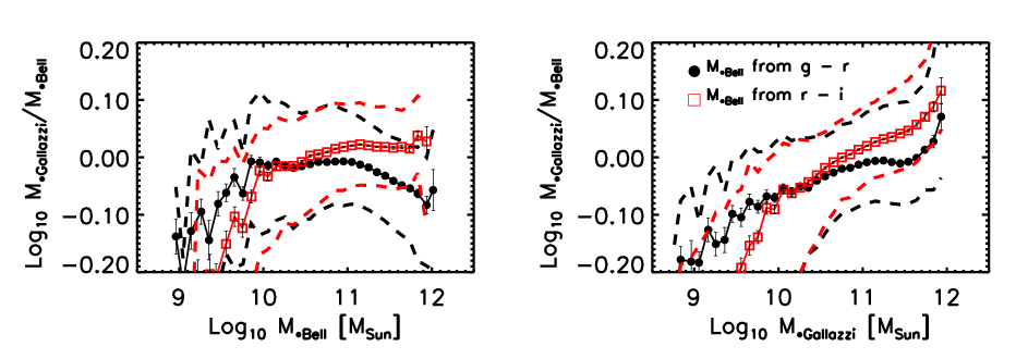


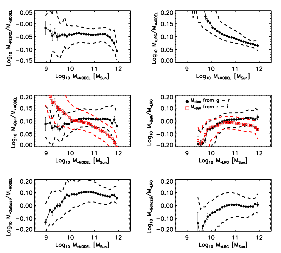


This section shows results from a study of how the different estimates compare with one another. We first show results for galaxies that have for two reasons. First, because this is expected to provide a sample dominated by massive galaxies, and these are expected to be more homogeneous. And second, we are particularly interested in studying the high mass end of the stellar mass function, because this is the end which is first observed in higher redshift datasets.
Figure 30 shows that the and estimates are in good agreement, although tends to be larger at . The sharp downturn at small masses is due to aperture effects. This is because is based on the model color; for otherwise similar galaxies, this samples the same fraction of a galaxy’s light (that within ) whatever its distance. On the other hand, is based on the light which enters the SDSS fiber (radius 1.5 arcsec); this samples a distance dependent fraction of the light of a galaxy. For small low mass galaxies which have significant disks, the fiber samples the bulge of the nearby objects, and the disks of the more distant ones. Since is larger for bulges than disks, the more distant objects of a given will have smaller . Here, of course, we have explicitly selected against disky galaxies, but color gradients will produce the same effect.
Figure 31 shows this effect explicitly: at fixed , the ratio decreases with increasing distance (this is a more dramatic effect for the lower mass systems in samples which include disks – see Figure 34). The panel on the right, which shows the angular size for objects of a fixed increasing at high , illustrates a curious selection effect (the upturn at higher redshift for the middle stellar mass bin, which is not present if when we study bins in luminosity). For a given , the highest redshift objects in a magnitude limited survey will be bluer; since color is primarily determined by velocity dispersion, these objects will have smaller than average velocity dispersions, and larger sizes. Although this is a small effect for the massive objects we have selected here, it is more dramatic in samples which include disks (as we show shortly; see Figure 34).
Figure 32 shows how these estimates compare with those from Blanton & Roweis (2007). The top left panel shows that is dex larger than (top left panel). Because the two estimates are based on the same mass-to-light ratio, this offset is entirely due to the fact that Petrosian magnitudes are 0.1 mags fainter than (the more realistic) model magnitudes. The middle left panel shows that is approximately independent of mass for , and strongly mass dependent for . But perhaps most importantly, note that is typically dex smaller than the based . This offset would have been even larger if we had compared to – the fairer comparison, because our here is based on the Petrosian magnitude. We argue shortly that this offset reflects the fact that the templates used to estimate are not appropriate for large masses. In contrast, is strongly mass dependent at small masses – this is because aperture effects matter for but not for . The behaviour at larger masses is a combination of aperture and template effects, but note again that is about 0.1 dex low.
The panels on the right show that fares much better. The top right panel shows that it is always substantially larger than , and the two panels below it show that is much more like and than is . Comparison with the corresponding panels on the left shows that much of the offset is removed, strongly suggesting that neither nor are reliable at the high mass end. This is not surprising – massive galaxies are expected to be old, so a 10 Gyr template should provide a more accurate mass estimate than ones that are restricted to ages of Gyrs or less. This will be important in Section 5. At the low mass end, is larger than either of the other estimates, suggesting that it overestimates the true mass. However, at these smaller masses, using exclusively produces masses which lie below and . This suggests that the LRG template remains the better description for a non-negligible fraction of low mass objects. Therefore, in practice, to use the Blanton & Roweis estimates, one must devise a method for choosing between and .
Figure 33 compares the different estimates of the stellar mass for the full sample. This gives similar results to when we restricted to , although the offsets are more dramatic. In this case, the selection effect associated with studying fixed makes the aperture effect associated with appear more complex than it really is: the large bump at the highest redshift associated with a given is not present when one studies objects at fixed luminosity (compare top and bottom panels of Figure 34).
Appendix B Tables
This Appendix provides tables which summarize the results of fitting equation (10) to the measured luminosity, stellar mass, size and velocity dispersion distributions shown in Figures 14–17. These measurements were obtained using cmodel magnitudes and sizes. We described our measurements by assuming that the intrinsic distributions have the form given by equation (9). The values between round brakets show the parameters obtained fitting equation (9) to the data ignoring measurement errors.
| Sample | Mpc-3 | Mpc-3 | |||
|---|---|---|---|---|---|
| HB09 | () | () | () | () | |
| CI 2.86 | () | () | () | () | |
| CI 2.6 | () | () | () | () | |
| All | () | () | () | () | |
| All () | () | () | () | () | |
| F07-E | |||||
| F07-S0 | |||||
| F07-Sa | |||||
| F07-Sb | |||||
| F07-Scd | |||||
| F07-All |
| Sample | Mpc-3 | Mpc-3 | |||
|---|---|---|---|---|---|
| HB09 | () | () | () | () | |
| CI 2.86 | () | () | () | () | |
| CI 2.6 | () | () | () | () | |
| All | () | () | () | () | |
| All () | () | () | () | () | |
| F07-E | |||||
| F07-S0 | |||||
| F07-Sa | |||||
| F07-Sb | |||||
| F07-Scd | |||||
| F07-All |
| Sample | Mpc-3 | /kpc | /kpc | ||
|---|---|---|---|---|---|
| HB09 | () | () | () | () | |
| CI 2.86 | () | () | () | () | |
| CI 2.6 | () | () | () | () | |
| All | () | () | () | () | |
| All ( kpc) | () | () | () | () | |
| F07-E | |||||
| F07-S0 | |||||
| F07-Sa | |||||
| F07-Sb | |||||
| F07-Scd | |||||
| F07-All |
| Sample | Mpc-3 | /km s-1 | /km s-1 | ||
|---|---|---|---|---|---|
| HB09 | () | () | () | () | |
| CI 2.86 | () | () | () | () | |
| CI 2.6 | () | () | () | () | |
| All | () | () | () | () | |
| All ( km s-1) | () | () | () | () | |
| F07-E | |||||
| F07-S0 | |||||
| F07-Sa | |||||
| F07-Sb | |||||
| F07-Scd | |||||
| F07-All |