Resonant Tunneling in Scalar Quantum Field Theory

In quantum mechanics (QM) the tunneling probability (or the transmission coefficient) of a particle incident on a barrier is typically exponentially suppressed. Somewhat surprisingly the addition of a second barrier can increase the tunneling probability for specific values of the particle’s energy. This enhancement in the tunneling probability, known as resonant tunneling, is due to constructive interference between different quantum paths of the particle through the barriers. Under the right conditions, the tunneling probability can reach unity. This is a very well understood phenomenon in quantum mechanics [1]. The first experimental verification of this phenomenon was the observation of negative differential resistance due to resonant tunneling in semiconductor heterostructures by [2]. In fact, this phenomenon has at least one industrial application in the form of resonant tunneling diodes [3].

Tunneling under a single barrier in quantum field theory (QFT) with a single scalar field is well understood, following the work of Coleman and others [4, 5]. Despite some arguments given in [6, 7], the issue of resonant tunneling in quantum field theory remains open [8, 9]. Recently, Sarangi, Shiu and Shlaer suggested that the functional Schrödinger method should allow one to study this resonant tunneling phenomenon [10]. In this paper, we apply this approach to study resonant tunneling in QFT with a single scalar field. We show that resonant tunneling in quantum field theory does occur and describe its properties. Following Coleman, we shall work in the thin-wall approximation.

Before going into any details, it is useful to give an intuitive argument why some effect like resonant tunneling should happen in QFT. Consider the following tunneling process for a potential shown in Figure 1. Let the tunneling rate from $A\to B$ be $\Gamma_{A\to B}=De^{-S}$, while its tunneling probability $T_{A\to B}=Ke^{-S}$, which are taken to be exponentially small. The prefactor $D$ or $K$ is of order unity with the proper dimension. Here we shall focus on the exponential factor. Suppose the tunneling rate from $B\to C$ is given by $\Gamma_{B\to C}$, which is also exponentially suppressed. Both $T_{A\to B}$ and $T_{B\to C}$ are evaluated using standard WKB method. A naive WKB analysis will suggest that the tunneling from $A\to C$ is doubly exponentially suppressed, i.e., $T_{A\to C}\approx T_{A\to B}T_{B\to C}$. However, this is not correct. Consider the typical time, namely $t_{A\to C}$, it takes to go from $A\to C$. It should be the sum of the time it takes to go from $A\to B$ plus the time it takes to go from $B\to C$. Since the typical time is simply the tunneling (or decay) time, which is the inverse of the rate of tunneling, we have

So it follows that

which is clearly not doubly suppressed. For the special case where $T=T_{A\to B}=T_{B\to C}$, we see that $T_{A\to C}\approx T/2$.

In QM, the exponential enhancement from $T_{A\to C}\approx T^{2}$ to $T/2$ is due to the resonant tunneling effect. At the resonances, $T_{A\to C}\approx 1$ while it is $\approx T^{2}$ off resonances. For a generic incoming wavefunction, with a spread in energy eigenvalues covering one or more resonances, this resonant effect yields $T_{A\to C}\approx T/2$, so the resonances typically dominate the tunneling process $A\to C$. More generally, the relations (1) and (2) are reproduced [6, 7]. Since the argument for (1) is general, it should apply in QFT as well as in QM. This suggests that some phenomenon like resonant tunneling must take place in QFT. The challenge is to find and understand it.

The functional Schrödinger method was developed by Gervais and Sakita [11] and Bitar and Chang [12]. It starts with the idea that tunneling is dominated by the most probable escape path (MPEP) developed by Banks, Bender and Wu [13]. In QFT with a single scalar field $\phi$, this path in the field space is described by $\phi_{0}({\bf x},\lambda)$, where ${\bf x}$ stands for the spatial coordinates and $\lambda$ is a parameter that parametrizes the field configurations in the MPEP. In Coleman’s Euclidean instanton approach, $\lambda$ is chosen to be the Euclidean time $\tau$, and the $O(4)$ symmetry of the instanton simplifies the analysis. On the other hand, the functional Schrödinger method allows one to make a different choice of $\lambda$. In the leading order WKB approximation, a generic choice leads one to a simple time-independent Schrödinger equation. It is not surprising that the resulting WKB formula for a single barrier tunneling process reproduces that of the Euclidean instanton approach. We shall present a step by step comparison so the equivalence of the two approaches is transparent. It is also obviously clear that the functional Schrödinger method is cumbersome by comparison. However, this method has the great advantage of being immediately generalizable to the double (actually multiple) barrier case. The underlying reason is that the same real parameter $\lambda$ parametrizes both the under barrier (Euclidean time $\tau$) and the classically allowed (Minkowski time $t$) regions.

For tunneling from vacuum $A$ to vacuum $C$ via the intermediate vacuum $B$ in scalar QFT, we consider the simultaneous nucleation of two bubbles, where the outside bubble separates $A$ from $B$ and the inside one separates $B$ from $C$. The functional Schrödinger method reduces this problem, in the leading WKB approximation, to a one-dimensional time-independent QM problem with $\lambda$ as the coordinate. The resulting double barrier potential in $\lambda$, namely $U(\lambda)$, allows us to borrow the QM analysis to show the existence of resonant tunneling. In the case when both bubbles grow classically after nucleation, the tunneling process from $A$ to $C$ will be completed. The tunneling rate is exponentially enhanced compared to the naive case. In the case where the inside bubble classically collapses back after its nucleation (because the bubble is too small for the difference in the vacuum energies to overcome the surface term due to the domain wall tension), only the tunneling from $A$ to $B$ is completed. Still the tunneling rate from $A$ to $B$ can be exponentially enhanced. To draw a distinction between these two different phenomena, we call the second process catalyzed tunneling. For catalyzed tunneling, vacuum $C$ plays the role of a catalyst.

The rest of this paper is organized as follows. Resonant tunneling in quantum mechanics is reviewed in Section 2. This review follows that in [1, 6] . As we shall see, the functional Schrödinger method reduces the QFT problem to a QM problem, so the resonant tunneling formalism in QM presented here goes over directly. In Section 3, we briefly review Coleman’s Euclidean action approach, following [4]. In Section 4, we present the functional Schrödinger method. Here, the discussion follows closely that given by Bitar and Chang [12, 14] and we need only the leading order WKB approximation. For the single-barrier tunneling process, we see how Coleman’s result is reproduced. In Section 5, we discuss the double-barrier case. This is the main section of the paper. Here we find that resonant tunneling can occur in two different ways. It can enhance the tunneling from vacuum $A$ to vacuum $C$ via the intermediate vacuum $B$, or it can enhance the tunneling from $A$ to $B$ in the presence of $C$. Section 6 contains some remarks. The appendix contains a discussion on the particular ansatz for $\phi$ used in the main text.

We first briefly review resonant tunneling in quantum mechanics. We consider a particle moving under the influence of a one-dimensional potential $V(x)$ with three vacua shown in Figure 1. Using the WKB approximation to solve the Schrödinger equation $H\psi=E\psi$ for the wavefunction of the particle $\psi(x)$ gives the linearly independent solutions

in the classically allowed region, where $k(x)=\sqrt{\frac{2m}{\hbar^{2}}(E-V(x))}$, and

in the classically forbidden region, where $\kappa(x)=\sqrt{\frac{2m}{\hbar^{2}}(V(x)-E)}$. A complete solution is given by $\psi(x)=\alpha_{L}\psi_{L}(x)+\alpha_{R}\psi_{R}(x)$ in the classically allowed region and $\psi(x)=\alpha_{+}\psi_{+}(x)+\alpha_{-}\psi_{-}(x)$ in the classically forbidden region. To find the tunneling probability from A to B we need to determine the relationship between the coefficients $\alpha_{L,R}$ of the components $\psi_{L,R}$ in vacuum A and the coefficients $\beta_{L,R}$ in vacuum B. The WKB connection formulae give

where $\Theta$ is given by

and $x_{1}$ and $x_{2}$ are the classical turning points. Setting $\beta_{L}=0$, the tunneling probablity is given by

Since $\Theta$ is typically exponentially large, $T_{A\to B}$ is exponentially small.

The same analysis gives the tunneling probability from $A$ to $C$, via $B$, as [1, 6],

where

and

with $x_{3}$ and $x_{4}$ the turning points on the barrier between B and C.

If $B$ has zero width, $W=0$ so $T_{A\rightarrow C}$ is very small,

However, if $W$ satisfies the quantization condition for the $n_{B}$th bound states in $B$,

then $\cos W=0$, and the tunneling probability approaches a small but not necessarily exponentially small value

This is the resonance effect. If $T_{A\rightarrow B}$ and $T_{B\rightarrow C}$ are very different, we see that $T_{A\rightarrow C}$ is given by the smaller of the ratios between $T_{A\rightarrow B}$ and $T_{B\rightarrow C}$. Suppose $T_{A\rightarrow B}\rightarrow T_{B\rightarrow C}$. Following (19), we see that $T_{A\rightarrow C}\rightarrow 1$ that is, the tunneling probability approaches unity. Notice that the existence of resonant tunneling effect here is independent of the detailed values of $\Theta$, $\Phi$, and $W$.

The above phenomenon is easy to understand in the Feynman path integral formalism. A typical tunneling path starts at $A$ and tunnels to $B$. It bounces back and forth $k$ times, where $k=0,1,2,...\infty$, before tunneling to $C$. When the Bohr-Sommerfeld quantization condition (18) is satisfied, all these paths interfere coherently, leading to the resulting resonant tunneling. On the other hand, if we raise the energy of the local minimum at B above the incoming energy $E$, then $W=0$ and $T_{A\rightarrow C}\sim T_{A\rightarrow B}T_{B\rightarrow C}$ which is typically doubly exponentially suppressed.

Single-barrier tunneling in quantum field theory was studied by [4] using the Euclidean instanton method. For concreteness, we will focus on the $(3+1)$-dimensional scalar field theory in Minkowski space described by the Lagrangian

with an asymmetric double well potential

with $B$ a small symmetry-breaking parameter. The potential at the false vacuum at $\phi=-c$ is zero, while the potential at the true vacuum at $\phi=+c$ is $-\epsilon\approx-2Bc$. The energy density difference between the two minima, namely $\epsilon$, is assumed to be small so that we may confine our analysis of this potential to the thin-wall regime. In the under-barrier (i.e., classically forbidden) region, one starts with the Euclidean action $S_{E}(\phi(\tau,{\bf x}))$ where $\tau$ is the Euclidean time. Solving the resulting Euclidean equation of motion for $\phi$ (with appropriate boundary conditions) and substituting it back into $S_{E}(\phi(\tau,{\bf x}))$ yields $S_{E}$. In the semi-classical limit [4] showed that the tunneling rate per unit volume is

where the subexponential prefactor $A$ studied in [5] will be unimportant for our purposes. The solution $\phi(\tau,{\bf x},R)$ to the Euclidean equation of motion is the familiar $O(4)$-symmetric domain-wall solution

where $\mu$ measures the (inverse) thickness of the domain wall,

so a relatively large $\mu$ (i.e., thin wall) is assumed. Here

and $R$ is the radius of the bubble. The bubble wall sits at $r=R$, so $\phi=+c$ for $r\ll R$ and $\phi=-c$ for $r\gg R$. That is, the bubble is surrounded by the false vacuum. It is useful to introduce the tension $S_{1}$ of the domain wall,

so the Euclidean action of this solution is now given by

where the first term is the four-volume times the energy density difference $\epsilon$ while the second term is the contribution of the domain wall. Setting the variation of this $S_{E}$ to zero yields

So the action is stationary for

which gives us

What happens to the bubble after nucleation? The bubble will behave in a way to decrease the energy $\mathcal{E}$, i.e., $d\mathcal{E}/dR<0$. It is easy to see that the bubble prefers to grow (classically) as long as

which is the case here. So, once the bubble is created with radius $\lambda_{c}$, the domain wall starts at rest and moves (classically) outwards, eventually attaining relativistic speed. Notice that the condition (28) is simply the classical energy conservation equation: at the moment right after bubble nucleation, the total energy $\mathcal{E}$ of the bubble and its interior equals to that of the original false vacuum in the region, which is zero.

Now let us introduce the functional Schrödinger method and apply it to the single barrier tunneling process discussed above in the same scalar QFT. In the semi-classical regime, a discrete set of classical paths, namely the most probable escape paths (MPEP) in configuration space give the dominant contributions to the vacuum tunneling rate [13, 11, 12]. Essentially this approximation allows us to reduce an infinite-dimensional quantum field theory calculation to a one-dimensional quantum mechanical computation. The effects of nearby paths can be included systematically in an $\hbar$ expansion, and were calculated to $O(\hbar^{2})$ in [11, 12], but will not be relevant for the rest of our analysis.

The Hamiltonian for a scalar field $\phi(t,{\bf x})$ where ${\bf x}$ denotes the three spatial directions is

where $V(\phi)$ is that given in (21). To quantize the field theory we use $[\dot{\phi}({\bf x}),\phi({\bf x}^{\prime})]=i\hbar\delta^{3}({\bf x}-{\bf x}^{\prime})$ to replace $\dot{\phi}$ with $-i\hbar\delta/\delta\phi$. This replacement allows us to write the time-independent functional Schrödinger equation as

where

and the eigenvalue $E$ is the energy of the system. As usual $\Psi(\phi({\bf x}))$ is the amplitude that gives a measure of the likelihood of the occurance of the field configuration $\phi({\bf x})$.

With the ansatz $\Psi(\phi)=A\exp(-\frac{i}{\hbar}S(\phi))$ where $A$ is constant, the functional Schrödinger equation (33) becomes

Expanding $S(\phi)$ in powers of $\hbar$, $S(\phi)=S_{(0)}(\phi)+\hbar S_{(1)}(\phi)+...$, and comparing terms with equal powers of $\hbar$ the functional Schrödinger equation (35) yields

The infinite set of nonlinear equations (36) on an infinite-dimensional configuration space can be reduced to a one-dimensional equation in the leading approximation. For our purpose here, we shall focus on $S_{(0)}$ and ignore the higher-order corrections $S_{(1)}$, $S_{(2)}$, etc. The essential idea is that there is a trajectory in the configuration space of $\phi({\bf x})$, known as the most probable escape path (MPEP), perpendicular to which the variation of $S_{(0)}$ vanishes, and along which the variation of $S_{(0)}$ is nonvanishing. We use $\lambda$ to parametrize this path in the configuration space of $\phi(x)$, so the MPEP is $\phi({\bf x},\lambda)$. This MPEP satisfies

Along the MPEP, we have

so $C(\lambda)$ is determined and we have

We now define the effective potential $U(\lambda)=U(\phi({\bf x},\lambda))$, so

then the classically allowed regions have $U(\phi_{0}({\bf x},\lambda))<E$ and the classically forbidden regions have $U(\phi_{0}({\bf x},\lambda))>E$.

Using the zeroth-order equation in (36) with (39) we find the WKB equation

To find the WKB wavefunctional it is sometimes useful to rewrite (41) in terms of the path length $ds$ in the configuration space. This path length is defined by

That is, choosing $s$ to parametrize the MPEP, (41) simplifies to

Now let us consider first the classically forbidden region, $U(\phi({\bf x},s))>E$. The solution to (43) is

where $\lambda_{t1}$ and $\lambda_{t2}$ are the turning points. Treating both $\frac{ds}{d\lambda}(\phi({\bf x},\lambda))$ (42) and $U(\phi({\bf x},\lambda))$ (40) as functionals of $\phi$, the Euler-Lagrange equation for $\phi({\bf x},\lambda)$ follows from setting the variation of $S_{(0)}$ to zero. It turns out that the resulting equation of motion derived from (44) simplifies considerably if we choose $\tau$ as the parameter where

With $\tau$ as the parameter, setting the variation of (44) equal to zero now yields

Here $\tau$ simply plays the role of Euclidean time, and (46) is simply the Euclidean equation of motion for $\phi({\bf x},\tau)$. Once we obtain the solution for $\phi({\bf x},\tau)$, we insert this solution into (44) to obtain the value $S_{0}$ for $S_{(0)}$. So we see that the functional Schrödinger method leads both to a determination of $S_{0}$ along the MPEP and an equation that determines MPEP, namely, $\phi_{0}({\bf x},\tau)$ itself. The subscript “0” indicates that it is the MPEP in the leading WKB approximation. The equation (46) has $O(4)$ symmetry, so it reproduces the familiar $O(4)$ symmetric domain-wall solution (23) in the thin-wall approximation ($r$ is the four-dimensional radial coordinate, $r^{2}=\tau^{2}+|{\bf x}|^{2}$),

after imposing the boundary conditions, $\phi\to-c$ as $r\to\infty$ and $\phi\to+c$ as $r\to 0$ and $\frac{d\phi(0)}{dr}=0$. Recall that $\lambda_{c}$ is the critical radius of the bubble given by (29).

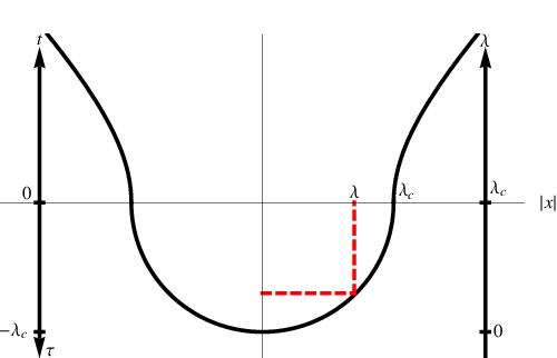
For our purpose, it is now convenient to introduce the parameter $\lambda$

which is the spatial radius of the bubble as shown in Figure 2. Here $\phi_{0}({\bf x},\lambda)=0$ for $\lambda<0$. For $\lambda_{c}>\lambda>0$ and near the domain wall at $r=\sqrt{{|{\bf x}|}^{2}+\tau^{2}}$, we have $r-\lambda_{c}\approx\pm({|{\bf x}|}^{2}-\lambda^{2})/(2\lambda_{c})\approx\pm({|{\bf x}|}\pm\lambda)\lambda/\lambda_{c}$. The corrections introduced by this approximation are exponentially suppressed far from the domain wall, so we can express the $O(4)$ symmetric solution (47) as,

This MPEP solution is plotted in Figure 3. (Slight care is needed for $\lambda\approx 0$, in which case, we simply go back to (47).) For $\lambda<0$ the solution is the false vacuum $\phi_{0}({\bf x},\lambda)=-c$ . As $\lambda>0$ increases, quantum fluctuation tends to fluctuate towards the true vacuum. At $\lambda=\lambda_{c}$, the bubble is created, which then evolves classically for $\lambda>\lambda_{c}$.

We have effectively reduced the WKB wavefunctional in the classically forbidden region to a WKB wavefunction which can be written using (44) as

where $m(\lambda)$ is obtained by substituting the MPEP $\phi_{0}({\bf x},\lambda)$ (49) into $m(\phi({\bf x},\lambda))$,

Here $m(\lambda)$ is the effective mass, which is manifestly positive, and the second equality is obtained in the thin-wall approximation. It is also straightforward to evaluate $U(\lambda)$ by substituting MPEP $\phi_{0}({\bf x},\lambda)$ (49) into $U(\phi({\bf x},\lambda))$ (40),

This approximation for $U(\lambda)$ is plotted in Figure 5. The classically forbidden region for zero-energy tunneling is $0<\lambda<\lambda_{c}$. As mentioned above, $\phi_{0}({\bf x},\lambda)$ (49) needs correction for $\lambda\sim 0$. The more accurate $U(\lambda)$ (the blue dotted curve) is also shown in Figure 5. However, this difference is not important for our analysis here.

Given $m(\lambda)$ (51) and $U(\lambda)$ (52), the tunneling problem in QFT has been reduced to a one-dimensional time-independent QM problem. We can now perform the integral in the exponent in (50) and obtain, for $E=0$,

which reproduces (30). (The factor of two difference is because, here, we are evaluating the exponent of the tunneling amplitude instead of the tunneling rate.) This result is completely expected since the expression (30) is obtained by integrating the Langrangian density with the $O(4)$ symmetric solution (47) or (23) in polar coordinates while here we are performing the same integral, first in the spatial coordinates $x$ and then in the $\lambda$ (or equivalently in $\tau$) coordinate. For an $O(4)$ symmetric solution, the latter approach is unnecessarily cumbersome.

So, before moving on, let us give a preview of the advantage of the functional Schrödinger method. This will also shed light on the underlying physics. In the classically allowed regions, similar arguments lead to the following $S_{(0)}$,

Similar to the previous case, the Euler-Lagrange equation of motion for $\phi$ simplifies if we choose the parameter $t$ such that

so setting the variation of $S_{(0)}$ with respect to $\phi({\bf x},t)$ to zero leads to

where $t$ is simply the normal time, and this is simply the equation of motion for $\phi({\bf x},t)$ in Minkowski space, $t\geq 0$. Now, instead of $t$, let us choose $\lambda$ as the parameter, where

which gives us ($\dot{\lambda}=d\lambda/dt$),

which is simply the Lorentz factor. Substituting this into the path (49), we obtain, for $\lambda>\lambda_{c}$,

so the classical path $\phi_{0}({\bf x},\lambda)$ now describes an expanding nucleation bubble, as its physical radius $\lambda$ increases towards the limiting speed $\dot{\lambda}=1$, with the proper Lorentz factor automatically included, and the effective tension now given by $S_{1}/{\sqrt{1-{\dot{\lambda}}^{2}}}$.

So we see that $\phi_{0}({\bf x},\lambda)$ for real $\lambda$ spanning $\infty>\lambda>-\infty$ works equally well for classically allowed as well as classically forbidden regions. In summary, $\phi_{0}({\bf x},\lambda)=-c$ for $\lambda<0$, when $\phi$ stays in the false vacuum. For $\lambda_{c}\geq\lambda>0$, $\phi_{0}({\bf x},\lambda)$ describes the “averaged” quantum fluctuation that corresponds to the MPEP for the tunneling process under the potential barrier. The $|{\bf x}|<\lambda$ region has fluctuated to the true vacuum, which is separated from the false vacuum region by a domain wall at $|{\bf x}|=\lambda$. Finally, for $\lambda\geq\lambda_{c}$, $\phi_{0}({\bf x},\lambda)$ describes the classical propagation of the nucleation bubble. The advantage here is that a single real parameter describes the whole system. The problem has been reduced to that of a time-independent one-dimensional (i.e., the $\lambda$ coordinate here) quantum mechanical system of a particle with position-dependent mass $m(\lambda)$ (51) and a potential $U(\lambda)$ (40) which has a barrier ($\lambda_{c}\geq\lambda>0$) that separates the two classically allowed regions. In general, the position-dependent mass complicates the quantization of the position variable. However, at leading order in the WKB approximation, such a complication does not arise.

The above discussion introduces the functional Schrödinger method and its applications to the tunneling process at leading order in $\hbar$. It reduces the tunneling process in an infinite-dimensional field configuration space to a one-dimensional quantum mechanical tunneling problem. The essential difference between tunneling in field theory discussed in Section 4 and in quantum mechanics discussed in Section 2 is that in field theory one should first find the MPEP, namely $\phi_{0}({\bf x},\lambda)$, and then obtain the effective potential $U(\lambda)$ (40) and the effective mass $m(\lambda)$ (51). We have extended the MPEP to include regions where classical motion is allowed.

References

- [1] See e.g., E. Merzbacher, Chapter 7 in Quantum Mechanics, 2nd edition, John Wiley, 1970.
- [2] L. L. Chang, L. Esaki, and R. Tsu, “Resonant tunneling in semiconductor double barriers,” Appl. Phys. Lett. 24, 593 (1974).
- [3] E.g., Wikipedia.
- [4] S. R. Coleman, “The Fate Of The False Vacuum. 1. Semiclassical Theory,” Phys. Rev. D 15, 2929 (1977) [Erratum-ibid. D 16, 1248 (1977)].
- [5] C. G. . Callan and S. R. Coleman, “The Fate Of The False Vacuum. 2. First Quantum Corrections,” Phys. Rev. D 16, 1762 (1977).
- [6] S. H. H. Tye, “A new view of the cosmic landscape,” arXiv:hep-th/0611148.
- [7] S.-H. H. Tye, “A Renormalization Group Approach to the Cosmological Constant Problem,” arXiv:0708.4374 [hep-th].
- [8] E. J. Copeland, A. Padilla and P. M. Saffin, “No resonant tunneling in standard scalar quantum field theory,” JHEP 0801, 066 (2008) [arXiv:0709.0261 [hep-th]].
- [9] P. M. Saffin, A. Padilla and E. J. Copeland, “Decay of an inhomogeneous state via resonant tunnelling,” JHEP 0809, 055 (2008) [arXiv:0804.3801 [hep-th]].
- [10] S. Sarangi, G. Shiu and B. Shlaer, “Rapid Tunneling and Percolation in the Landscape,” Int. J. Mod. Phys. A 24, 741 (2009) [arXiv:0708.4375 [hep-th]].
- [11] J. L. Gervais and B. Sakita, “WKB wave function for systems with many degrees of freedom: A unified view of solitons and pseudoparticles,” Phys. Rev. D 16, 3507 (1977).
- [12] K. M. Bitar and S.-J. Chang, “Vacuum Tunneling And Fluctuations Around A Most Probable Escape Path,” Phys. Rev. D 18, 435 (1978); “Vacuum Tunneling Of Gauge Theory In Minkowski Space,” Phys. Rev. D 17, 486 (1978).
- [13] T. Banks, C. M. Bender and T. T. Wu, “Coupled anharmonic oscillators. 1. Equal mass case,” Phys. Rev. D 8, 3346 (1973);
- [14] S.-J. Chang, Chapter 9 in Introduction to Quantum Field Theory, World Scientific, 1990.