Probing the anisotropies of a stochastic gravitational-wave background using a network of ground-based laser interferometers
Abstract
We present a maximum-likelihood analysis for estimating the angular distribution of power in an anisotropic stochastic gravitational-wave background using ground-based laser interferometers. The standard isotropic and gravitational-wave radiometer searches (optimal for point sources) are recovered as special limiting cases. The angular distribution can be decomposed with respect to any set of basis functions on the sky, and the single-baseline, cross-correlation analysis is easily extended to a network of three or more detectors—that is, to multiple baselines. A spherical harmonic decomposition, which provides maximum-likelihood estimates of the multipole moments of the gravitational-wave sky, is described in detail. We also discuss: (i) the covariance matrix of the estimators and its relationship to the detector response of a network of interferometers, (ii) a singular-value decomposition method for regularizing the deconvolution of the detector response from the measured sky map, (iii) the expected increase in sensitivity obtained by including multiple baselines, and (iv) the numerical results of this method when applied to simulated data consisting of both point-like and diffuse sources. Comparisions between this general method and the standard isotropic and radiometer searches are given throughout, to make contact with the existing literature on stochastic background searches.
pacs
95.55.YmI INTRODUCTION
Data from the laser interferometric gravitational-wave detectors LIGO [1, 2, 3, 4], Virgo [5, 6], and GEO [7, 8] are currently being analysed for the presence of gravitational waves from a variety of sources. These include signals from inspiraling and coalescing compact binaries (for example, neutron stars and/or stellar mass black holes) [9, 10, 11, 12], continuous gravitational waves from quasi-periodic sources such as pulsars [13, 14, 15, 16], and bursts of gravitational radiation associated with gamma-ray bursts [17, 18, 19], core-collapse supernovae, or other violent events [20]. In addition, searches are ongoing for the presence of a background of stochastic gravitational radiation of either astrophysical or cosmological origin [21, 22, 23], whose detection might provide insights about the very early universe [24], well before the production of the cosmic microwave background [25].
Although no direct detections of gravitational waves have been made to date, the most recent data taken are of unprecented sensitivity [26, 13, 17], leading to upper limits on gravitational-wave strengths that are competitive with or surpass those from electromagnetic or particle physics observations. Of particular note is the upper limit on the strength of a gravitational-wave signal from the Crab pulsar [27], which is a factor of 1.6 lower than the corresponding limit inferred from electromagnetic pulsar spin-down observations [28]. Also, the current direct limit on the strength of an isotropic stochastic gravitational-wave background at [26] (at 95% confidence) has surpassed bounds set by considerations from Big Bang Nucleosynthesis [24] and from the microwave background [29].
In this paper, we describe an analysis method that estimates the angular distribution of power in an anisotropic stochastic gravitational-wave background. This method includes both the standard isotropic [30, 31, 23] and gravitational-wave radiometer searches [32, 21] (optimal for point sources) as special limiting cases. (For our purposes anisotropic is taken to mean not necessarily isotropic.) Similar to the radiometer technique, the method presented here looks for modulations in the gravitational-wave signal induced by the Earth’s rotational motion relative to an anisotropic background. The method provides maximum-likelihood estimates of the angular distribution of gravitational-wave power , decomposed with respect to some set of basis functions on the sky. By choosing a pixel basis , we recover the results of the radiometer method discussed in [32, 21]. By choosing the spherical harmonics basis defined with respect to the Earth’s rotational axis, we obtain maximum-likelihood estimates of the multipole moments of the gravitational-wave sky. This basis is particularly convenient as the standard isotropic analysis corresponds to simply restricting attention to the monopole moment , while the point-source radiometer results are well-approximated by choosing a sufficiently large value of (), appropriate for the diffraction-limited beam pattern at kHz. In addition, the use of spherical harmonics simplifies the problem of removing the ‘smearing’ effects of the beam pattern from the measured sky map (that is, deconvolution of the dirty map), given the smaller number of elements and symmetries of the beam pattern matrix with respect to the indices. The problem of deconvolving a cross-correlated gravitational-wave signal from the interferometers’ beam pattern in the spherical harmonic basis has been described in [33]. We address this problem in detail in section IV. We further note that the spherical harmonic basis is useful for the efficient analysis of cross-correlated data in a variety of applications including searches for transient gravitational-wave sources [34].
Regardless of basis, the method described here is easily extended to work with a network or three or more detectors with uncorrelated detector noise, by simply adding the individual baseline beam patterns and dirty maps before deconvolution. A multi-baseline analysis improves the overall sensitivity of the search by reducing the variances of the individual estimators, and provides a natural way of regularising the deconvolution of the dirty map; the beam pattern matrix has fewer null (or nearly null) directions for multiple baselines and is thus more stable during inversion.
The structure of the rest of the paper is the following: In section II, we briefly review the statistical properties of an anisotropic background, and show how a generalized overlap reduction function arises in a cross-correlation search for such a background. In section III we derive the optimal estimators of the angular distribution of the gravitational-wave power, starting from the likelihood function for cross-correlated data. We explicitly construct the beam pattern matrix, and discuss its relation to the covariance matrix of the estimated . Section IV describes details of the data analysis implementation and issues related to deconvolution and regularisation. It also briefly describes how to extend the analysis to a network of three or more detectors, and the expected increase in sensitivity from using multiple baselines. In section V we present numerical results of the method applied to simulated data. We consider both point-like and diffuse-source injections, and compare the extracted and injected sky-maps. Finally, in section VI we summarize our results. We also include three appendices: Appendices A and B contain definitions of the spherical harmonics and some useful identities relating different multipole moments, beam pattern matrix components, etc.; Appendix C defines a related detection statistic that assumes a particular distribution of (normalized) angular distribution functions on the sky.
II GRAVITATIONAL-WAVE BACKGROUNDS
Stochastic gravitational-waves are produced by the superposition of a large number of weak, independent, unresolved gravitational-wave sources. The signal can be either cosmological or astrophysical in nature, leading to different expected characteristics: (i) A cosmological background, consisting e.g., of remnant gravitational waves left over from the very early universe, is expected to be predominantly isotropic, similar to that of the 2.73 K temperature distribution of the cosmic microwave background. (ii) An astrophysical background, on the other hand, produced by more recent astrophysical events, such as early-phase compact binary inspiral or continuous radiation from pulsars (see, e.g., [35]), will most likely be anisotropic, following the spatial distribution of the sources. In addition, cosmological backgrounds are expected to have relatively smooth, monotonic power spectra (for example, falling off close to for standard inflationary models) [36], while astrophysical backgrounds are expected to have power peaked at some characteristic frequency. Not surprisingly, to optimally search for these different signals requires different search algorithms, adapted for the angular distribution and spectral properties of the source. In this section, we describe how the anistropy of a stochastic gravitational-wave background manifests itself in the statistical properties of the signal, and in the expected value of the cross-correlation of the output of two detectors. The following sections then describe how one can search for such a signature in the measured data.
II.1 Statistical properties
In the transverse-traceless gauge, the metric perturbations due to a stochastic gravitational-wave background can be written as a superposition of plane waves having frequency and propagating in the direction :
| (1) |
where are the gravitational-wave polarization tensors. (Summation over polarization indices is understood.) In standard angular coordinates on the two-sphere , , we can write
| (2) | |||||
| (3) | |||||
| (4) |
so that forms a right-handed system of unit vectors. We can then define the two () polarization tensors to be
| (5) | |||||
| (6) |
Note that there is a rotational degree of freedom in the definition of polarization tensors as one is free to rotate and by an angle in the plane orthogonal to . For a gravitational-wave source with a symmetry axis, such as an inspiralling binary, the angle can be interpreted as the polarization angle of the source. However, as we will assume that the stochastic background is unpolarized, there is no loss of generality in taking , so that the polarization tensors have the form given above.
The Fourier coefficients are complex functions that satisfy , since is real. For a stochastic gravitational-wave background these coefficients are random fields whose expectation values define the statistical properties of the background. Without loss of generality we can assume that the fields have zero mean:
| (7) |
We will also assume that the background is unpolarized, Gaussian, and stationary, but allow for an anisotropic distribution. The most general form of the quadratic expectation value satisfying these requirements is
| (8) |
where specifies both the spectral and angular distribution of the background. The factor of has been included so that for an isotropic background is the one-sided strain power, when summed over both polarizations. Given the above definitions, it follows that
| (9) |
where is the energy density contained in the frequency interval . Here is Hubble’s constant, and is the critical energy density needed to close the universe. (To prove Eq. (9), one should write in terms of an expectation value of the product of the time derivatives of the metric perturbations , and then expand the metric perturbations in terms of the plane wave components as in Eq. (1), using Eq. (8) to evaluate the expectation value; see, e.g., [37, 38].) Thus, the energy density in a stochastic gravitational-wave background has contributions from all parts of the sky as encoded in the all-sky integral of .
In what follows, we will assume that can be factorized into a product of two functions
| (10) |
where is a dimensionless function of frequency, normalized so that , where is a reference frequency, typically taken to equal (a frequency in LIGO’s most sensitive band). specifies the angular distribution of gravitational-wave power, and its spectral shape. This factorization does not amount to a loss of generality if one restricts attention to small enough frequency bands. For our analysis, we will assume that
| (11) |
where is a power-law index which we fix (for example, for constant strain power). Using Eqs. (9) and (10), one can show that this assumption for is consistent with
| (12) |
where is the fractional energy density in gravitational waves evaluated at the reference frequency .
The angular distribution function can be expanded in terms of a set of basis functions on the two-sphere according to
| (13) |
where summation (or integration) over is understood, and
| (14) | |||||
| (15) |
The choice of basis, in principle, should not affect the physical search results. However, in practice, such a choice can bear on computational costs of a search and also on the systematic errors affecting observations results, e.g., arising from the truncation order of the spherical-harmonic basis. For these reasons, we expect that while searching for gravitational-wave point sources, a decomposition with respect to a pixel basis
| (16) |
is the natural choice. For a diffuse background, e.g., dominated by a dipole or quadrupolar distribution, a spherical harmonic decomposition may be the better choice:
| (17) | |||||
| (18) |
where the second equality follows from our normalization convention for the (see Appendix A). Note that the pixel basis coefficients, , have units of whereas the coefficients in the spherical harmonics basis, , have units of . This normalization convention also implies
| (19) |
Note that only the monopole moment contributes to (and hence to ) as all higher-order multipole moments give zero when integrated over the sky.
II.2 Overlap factor
We will denote the time-series output of two detectors by
| (20) |
where is the detector noise and is its response to a gravitational-wave background:
| (21) |
Here
| (22) |
is the detector response function, which encodes the directional sensitivity of detector to a plane-polarized gravitational wave propagating in direction and specifies the location of interferometer . (The absolute value plotted as function of direction is called the detector antenna pattern.) The detector tensor is
| (23) |
where , are unit vectors pointing along the interferometer arms for detector . The vectors , , and are all time-dependent due to the Earth’s rotation. (We are using equatorial coordinates, with the spatial origin at the center of the Earth, -axis pointing along the Earth’s rotation axis, and -axis pointing in the direction of the vernal equinox.)
Given a time-series , we define its short-term Fourier transform by
| (24) |
where is much greater than the light-travel time between any pair of detectors, but is small enough that the the detector response function and detector location do not vary significantly with time over the interval . Typical values of are from a few tens of seconds to a few hundred seconds. The cross-correlation between the output of the two detectors is then defined in terms of these short Fourier transforms as
| (25) |
The factor of 2 is a convention consistent with the definition of one-sided power spectra, so that the total cross-power for a particular time is given by integrating over positive frequencies. These cross-spectra are the starting point for the maximum-likelihood analysis described in the following section.
If the noise at the two detectors is uncorrelated—a reasonable assumption for spatially-separated detectors—then it follows that the expectation value of the cross-spectra depends only on the gravitational-wave signal components
| (26) |
Using Eqs. (8), (10), and the short-term Fourier transform of (21), one can then show that
| (27) |
where
| (28) |
The function is a geometric factor that takes into account the separation and relative orientation of the two detectors (see e.g., [39]). For an isotropic background, , where
| (29) |
is the standard overlap reduction function [40, 41]. The factor of is a normalization constant chosen so that for all frequencies for a pair of coincident and coaligned interferometers with 90-degree opening angle between the interferometer arms. Note that is time-independent due to the all-sky integration.
For subsequent analysis, it will be convenient to rewrite the right-hand side of Eq. (27) in terms of an integral over the components of and with respect to a set of basis functions on the two-sphere
| (30) |
where
| (31) | |||||
| (32) |
Therefore, in the pixel basis, , one has
| (33) |
and in the spherical harmonics basis, , one gets
| (34) | |||||
| (35) |
Note that the above definition of differs from that (18) of by a complex conjugation, but it agrees with the convention used in [38]. The time-dependence of is particularly simple:
| (36) |
In addition, for an isotropic background, the above definitions imply for any .
III MAXIMUM-LIKELIHOOD ANALYSIS
In this section, we derive the maximum-likelihood estimators of the angular distribution of the stochastic gravitational-wave power. The analysis given below also makes clear the relationship between the covariance matrix of these estimators and the beam pattern matrix for the cross-correlation measurements. Since maximizing the likelihood is equivalent to minimizing the squared deviation of the estimators away from their expected values, the estimators so obtained are optimal in the sense of maximizing the expected signal-to-noise ratio of the estimators. Hence, the likelihood analysis reproduces the standard results of optimal filtering for the isotropic (e.g., [30, 31, 23]) and radiometer [32, 21] analyses without explicitly introducing a filter function in the construction of a statistic.
III.1 Maximum-likelihood estimators
The maximum likelihood analysis for an anisotropic stochastic background takes as its fundamental data vector the cross-spectra
| (37) |
evaluated at a set of discrete times and discrete (positive and negative) frequencies . As shown in the previous subsection, the expectation values of the cross-spectra are given by
| (38) |
The covariance matrix is given by
| (39) | |||||
| (40) |
where , are the one-sided power spectra of the detector output for time segment , which satisfy
| (41) | |||||
| (42) |
We have assumed that there is no cross-correlated noise, and that the cross-correlated and auto-correlated gravitational-wave signal power are much less than the detector noise power to obtain the approximate relations Eqs. (40) and (42).
Treating and the gravitational-wave spectral shape as known quantities, the likelihood function is then
| (43) |
where
| (44) |
Using Eqs. (38) and (40), we have
| (45) |
Since maximizing the likelihood with respect to is equivalent to minimizing chi-squared, one can show that the maximum likelihood estimators for the are given by
| (46) |
where
| (47) | |||
| (48) |
(We will adress the invertability of in section IV.) Note that the standard estimator of the strength of an isotropic stochastic background [30, 31, 23]
| (49) |
has the same form as the above, with playing the role of and the role of .
For later reference, we note that the minimum value of chi-squared is , which can be written explicitly as
| (50) |
Also, in analogy with what is done for cosmic microwave background experiments such as WMAP [42], we can construct estimators of the angular “power” spectra
| (51) |
by simply replacing with the estimators evaluated in the spherical harmonics basis—i.e.,
| (52) |
Note that the defined above are actually estimators of the squared angular power (since already has units of power), unlike the cosmic microwave background data for which the really do have units of power. Also, we will see in the next subsection that these estimators are biased. Unbiased estimators of the are given in equation (60).
III.2 Error estimates
If the spectral shape that we assumed for the signal model exactly matches that of the observed background, it is fairly easy to show that the estimators constructed above provide unbiased estimates of the angular distribution of gravitational-wave power:
| (53) |
This follows immediately from the fact that
| (54) |
which in turn shows that the are the components of the so-called ‘dirty’ map—i.e., represent the gravitational-wave power on the sky as seen through the beam matrix of the two detectors, . Equation (46) shows that by inverting , one obtains the components of the ‘clean’ map, . The process of going from the dirty map to the clean map is an example of deconvolution.
In addition, one can show in the weak-signal approximation that
| (55) | |||
| (56) |
Thus, is the covariance matrix of the dirty map , and is the covariance matrix of the clean map . A matrix like , whose inverse is the covariance matrix of the signal parameters, is often called a Fisher information matrix. An alternative definition of , illustrating its connection to the likelihood function, is
| (57) |
As is evident from the above expression, if one has several independent measurements (so that the combined likelihood is just a product of individual likelihoods), the matrices simply add.
Finally, using the above expressions for the expectation value and covariances of the , one can show that
| (58) | |||||
| (59) |
Note, in particular, that the estimators are biased. Unbiased estimators of the are given by
| (60) |
III.3 Decomposition in terms of pixel basis or spherical harmonics
The analysis presented above has been written in terms of the components and of and with respect to an arbitrary set of basis functions on the two-sphere. For most purposes, we will be interested in the components with respect to only two bases: The pixel basis, for which and and are given by (16) and (33), and the spherical harmonics basis, for which and and are given by (18) and (35). Each basis has its own set of advantages and disadvantages, which we briefly describe below.
In the pixel basis, is an estimate of the true gravitational-wave power coming from direction . It is a real quantity and should be non-negative. The quantity , on the other hand, is the power coming from direction as seen by the detector. It includes gravitational-wave power from other directions on the sky due to the finite acceptance of the beam pattern function, as well as from instrumental noise. The matrix connects the two via (54), and can be directly interpreted as a point spread function. It specifies how a point source at is spread to other points by the response of a pair of detectors.
In the spherical harmonics basis, the are estimates of the true multipole moments of the gravitational-wave power on the sky. The matrix , is no longer directly interpretable in terms of a point spread function, but it plays an analogous role as the inverse matrix specifies the correlations between the various multipole moment estimates.
In addition, the Fisher matrix has two symmetries: parity (see Eq. 90) and rotational symmetry around the z-axis. Since spherical harmonics respect these symmetries, this leads to some simplifications. Parity is an exact symmetry, because the only difference between gravitational-wave signals coming from antipodes is an opposite sign of the time shift between detectors. Therefore the detector noise, as expressed by the Fisher matrix, is identical for antipodes. This implies that for all odd (almost half of the matrix elements). Z-axis rotational symmetry is broken by daily variations in detector sensitivity, but still implies that for , i.e., is a block-diagonally dominant matrix. The pixel basis has no such symmetry.
Furthermore, in the spherical harmonics basis it is simple to specify a resolution cut-off by only allowing . This avoids over-sampling and reduces the number of required basis vectors. Also, since extending this cut-off to a larger does not affect the original basis vectors, it is straightforward to run the analysis with a higher resolution, and later do the matrix inversion at a lower resolution.
Finally, the computationally dominant part of the analysis is the calculation of the Fisher matrix. Since the Fisher matrix has elements, with the number of basis vectors, working in the spherical harmonics basis makes the analysis significantly more efficient. And the mentioned symmetries help to reduce the computational load even more.
IV IMPLEMENTATION AND ANALYSIS DETAILS
As shown in Sec. III.1, the maximum-likelihood estimators of the angular distribution of power in an anisotropic gravitational-wave background are given by
| (61) |
where are the components of the ‘dirty’ map (47), and are the components of the inverse of the beam pattern matrix (48). In this section, we describe: (i) some of the implementation details related to the calculation of and , (ii) a method for regularizing the inversion of , (iii) how to extend the single baseline analysis to a network of detectors, and (iv) a Bayesian model selection scheme for determining for the spherical harmonic decomposition. For concreteness we consider a network of detectors consisting of the LIGO interferometers H1 and L1 and the Virgo interferometer, V1.
IV.1 Calculating and
The components of the ‘dirty’ map and the beam pattern matrix are given by
| (62) | |||
| (63) |
These are the fundamental data products of this analysis from which and are then calculated (61). Although the various quantities entering and have already been defined in the previous two sections, we describe here in more detail how they are calculated in practice.
(i) is the assumed spectral shape of the gravitational-wave background (11). This is an input to the data analysis pipeline which we fix at the start of the analysis. The parameters and are the reference frequency and spectral index for the (assumed) power-law behavior of the gravitational-wave spectrum. For the analyses described later in this paper, we choose and , corresponding to constant strain power. Other values of and are, of course, possible. For example, corresponds to constant fractional energy density , which follows from Eq. (12).
(ii) are the cross-spectra of the data, calculated as a product of the short-term Fourier transforms of the time-series output of the two detectors, cf. Eqs. (25), (24). The time-series data are first downsampled to a few kilohertz (from 16384 Hz to 2048 Hz for LIGO; from 10000 Hz to 2000 Hz for Virgo), high-pass filtered above 40 Hz (to reduce contamination from low-frequency seismic noise), and then windowed (to avoid spectral leakage of strong instrumental lines), before being discrete-Fourier-transformed to the frequency domain. As is typically of order 100 s ( for the simulations that we will describe in Sec. V), the frequency resolution of and is of order , which is much finer than what is needed for the other frequency-series , , and , which are typically taken to have a frequency resolution . Hence, to match , we average together several frequency bins of . This averaging or “coarse graining” has also been used for previous stochastic searches, see e.g. [30]. It is a technique used to avoid unnecessary frequency resolution, especially in and .
(iii) are the power spectra associated with the individual () detector outputs (41). We use Welch’s modified periodogram method to estimate the power spectra, averaging together periodograms from 4-sec long, 50% overlapping, Hann-windowed data, which are taken from the two time segments immediately preceding and following—but not including—the analyis segment. (The 4-sec data stretches corresponds to the Hz frequency resolution mentioned earlier.) This technique greatly reduces a bias that would otherwise result from non-zero covariance between and .
For an actual analysis of real data, one needs to consider the possibility of short-term variations in the detector noise that are not consistent between the analysis segment and the two neighboring segments from which the were estimated. For the simulations that we will describe in Sec. V, the data were stationary, so no consistency cut needed to be applied.
(iv) are the components of the overlap factor defined by Eqs. (28), (33), (35). These are geometric factors that encode the relative separation and orientation of the two detectors, as specified by the detector response functions (22), (23). In the pixel basis, the components can be efficiently calculated by using one Fast Fourier Transform, and reading out the resulting cross-correlation time series at the time shift corresponding to each pixel [43, 21]. In the spherical harmonics basis, the components can be efficiently calculated using analytic expressions derived in [38]. In particular, the authors in [38] show that for sidereal time , one can write as a simple linear combination of spherical bessel functions (for even) or (for odd), where depends on the relative separation of the detectors . The coefficients of the linear combinations are complex numbers that depend on the relative orientation of the detectors. Explicit expressions for a few of the for the LIGO Hanford-Livingston pair are given below:
| (64) | ||||
| (65) | ||||
| (66) |
(Note that the numerical coefficients above do not agree with those in [38], due to an overall normalisation by and phase factor , where is the angle between the separation vector between the LIGO Hanford and Livingston detectors and the Greenwich meridian.) For arbitrary sidereal times , one uses Eq. (36), which follows from the dependence of the spherical harmonics . Here are related to the equatorial coordinates (ra,dec) via and .
IV.2 Deconvolution and regularization
Equation (61) is a formal description for estimating the angular structure of a gravitational-wave background. We refer to this as deconvolution since it tries to remove the smoothing introduced by the point spread function. Deconvolution requires inverting the Fisher matrix . However, in practice, the Fisher matrix is somewhat ill-conditioned. There are two reasons for this.
First, the detector pair is diffraction limited. Thus, as we choose a basis with higher spatial resolution, the condition number of the Fisher matrix gets worse, resulting in a reduced signal-to-noise ratio for the deconvolved map. We can address this by picking a basis with a reasonable resolution cut-off, which makes the spherical harmonics basis set with a natural candidate.
Second, there are certain power distributions to which the detector pair is essentially blind. For those distributions positive and negative contributions from different sky locations to the total cross-correlation essentially cancel. Mathematically they are described by
| (67) |
i.e., they are the eigenfunctions of the Fisher matrix with the smallest eigenvalues. These eigenfunctions tend to have -axis rotational symmetry because the detector pair is rotating with the Earth. However this symmetry can be broken by daily variations in detector sensitivity. To address this second issue, we have chosen to use a singular value decomposition (SVD) regularization scheme, which we describe in some detail below.
Since is Hermitian, its SVD has the form
| (68) |
where is a unitary matrix and is a diagonal matrix with non-negative entries (the eigenvalues of ). Without loss of generality we can further assume that the diagonal elements of are sorted from the largest to smallest values. Then the problematic modes according to Eq. (67) correspond to the last entries of the diagonal of . Figure 1 shows the relative size of the eigenvalues of a typical matrix in the spherical harmonics basis (with ), taken from the no-injection simulation of Section V. We can now set a threshold on the size of the eigenvalues, setting all eigenvalues to infinity (their inverse to zero), or alternatively to . Using this modified matrix we can then define the regularized as
| (69) |
and its inverse as
| (70) |
The threshold is chosen by weighting the quality of the deconvolution (larger point spread function for higher values of ) against the addition of noise due to poorly measured modes (lower values of ). While one can make this trade-off argument more quantitative, the choice will be somewhat influenced by the spatial shapes one is looking for. For the purpose of this paper, we simply chose to keep of all eigenmodes, and set all the small eigenvalues equal to . This is somewhat arbitrary, but a reasonable choice to get rid of the extremely small eigenvalues of a typical Fisher matrix (Figure 1). As can be seen in Sec. V, this choice allows for a reasonable recovery of simulated injections.
Using this regularization scheme has two side effects that need to be mentioned. First, Eq. (46) is replaced by
| (71) |
Thus the expectation value of is
| (72) |
This constitutes a bias in the estimator, which is expected since we chose to ignore the modes of that are poorly measured. Under the assumption that we know the shape of the source this bias can be calculated. Assuming the signal consists of point sources, Figure 2 shows the size of that bias as a function of sky position. Second, the covariance matrix of (in the weak-signal approximation) is now given by
| (73) |
Finally, we note that adding additional detector pairs with different baselines can, to a certain degree, act as a natural regulator, simply because one detector network might be more sensitive to a particular mode than another as illustrated in Figure 1. This is described in more detail in the following subsection.


IV.3 Multiple baselines
As shown explicitly in [32] for the case of the directed radiometer method, the above analysis can easily be extended to a network of three or more detectors with uncorrelated detector noise. One simply adds the dirty maps and Fisher matrices for each distinct detector pair :
| (74) |
where the subscript signifies a network of baselines. This follows from extending the likelihood formulation in Sec. III to include sums over baselines as well as frequency and time. The maximum-likelihood estimators then retain the same form as for the single baseline case, namely
| (75) |
This follows immediately from Eq. 57.
Different baselines in the network partly complement each other and help fill gaps in sensitivity present in individual baselines pairs. This has an important consequence. The sensitivity gaps correspond to degeneracies in the Fisher information matrix, which make it hard to estimate the true stochastic background. By filling these gaps the network acts as a natural regularizer, as illustrated in Fig. 1.


Our next step is to quantify how the natural network regularization and the SVD regularization reduce the error in estimating the spherical harmonic components. The full covariance matrix of the estimated multipoles is the best measure of estimation error, but it is inconvenient to compare covariance matrices. Rather, we use the standard deviation of each multipole as our figure of merit for estimation error:
| (76) |
for unregularized estimators, and
| (77) |
for regularized estimators (no summation over in either of these two formulas). We plot the standard deviations for each multipole for both unregularized and regularized estimators in Fig. 3 and Fig. 4, respectively. Both of these figures indicate that multiple baselines vastly reduce the estimation error. In addition, Fig. 4 illustrates that though the estimation error is minimized when both the network and SVD regularization are present, the SVD regularization alone can significantly reduce the estimation error (to just more than the regularized network error) for the LIGO only baseline. Thus, even if one interferometer is not unusable for some period, the regularized spherical harmonic moment estimators for the remaining baseline can still provide reasonable results.
IV.4 Model selection for spherical harmonic decomposition
In addition to choosing the cutoff for the SVD regularization of the Fisher matrix (as described in Sec. IV.2), one needs to specify the value of , the maximum value of the spherical harmonic index used in the spherical harmonic decomposition. Choosing fixes the total number of multipole moments , and hence defines the signal model. Larger values of mean finer angular resolution of the sky maps and more parameters available to fit the data. But since the estimators are correlated with one another, increasing the number of parameters simultaneously increases the uncertainty associated with each parameter. Thus, there is a tradeoff between accurately modeling the data (more parameters) and minimizing uncertainties (fewer parameters). In this subsection we outline how Bayesian model selection can be used to fix . (This discussion is meant to motivate future study as we do not implement a model selection scheme in this work.)
Bayesian model selection (see, e.g., [44]) is a framework in which the data themselves determine which signal model is most appropriate. The basic idea is to compare the various models (e.g., and ) by computing the ratio of the probability of the models given the data . By Bayes’ theorem, we have
| (78) |
where and are the a priori probabilities of the models, and and are the likelihood functions for the data given the two models. The ratio of the likelihoods is known as the “Bayes factor” (see, e.g., [44]). If there is no a priori reason to prefer one model over the other (as is often the case), then , implying that the posterior odds is just the ratio of the likelihood functions, . Since a given model often involves a set of parameters , calculating the likelihood of the data for a given model requires marginalizing over the possible values of these parameters—i.e.,
| (79) |
where is the prior probability distribution of the parameters for that model.
In situations where the data is informative—i.e., when the likelihood function is peaked relative to the prior —we have the approximate relation
| (80) |
where is the value of that maximizes the likelihood, is the range of parameter values over which the likelihood is peaked, and is the full range of parameter values. The factor penalizes a model that uses more parameter space volume than needed to fit the data. This factor can be understood in terms of Occam’s razor, which says that everything else being equal, simpler models that can adequately fit the data are preferred.
For example, if we ignore the subtleties described in Sec. IV.2 related to the inversion of the Fisher matrix , an map (961 parameters) will always fit the data better than an map (36 parameters) in the sense of having a larger value of . One can imagine, however, a stochastic background characterized by up to only . In that case, an fit would introduce a great many unnecessary parameters, which means a much smaller value of offsetting the larger value of . In addition, since the multipole moment estimators for different and are correlated with one another, choosing a large value of would have the undesirable effect of worsening the uncertainty associated with the up to .
In the context of our search for an anisotropic stochastic gravitational-wave background, the model is that a signal is present having multipole moments up to . The data are the measured cross-spectra , and the likelihood function is given by Eq. (43), where the signal model is defined by multipole moments up to . Thus, the quantity we need to calculate is the marginalized likelihood
| (81) |
where are the prior probability distributions for the multipole moments. Since the parameter space is large (a total of parameters), sophisticated Markov Chain Monte Carlo techniques (see [45]) may be required to numerically evaluate this integral. If the data turn out to be informative, then one has the much simpler expression
| (82) |
where are the maximum-likelihood estimators given by Eq. (46), and are characteristic widths of the prior distributions. Whether or not one can use this approximation depends on the actual data and the choice of priors. In practice, it may be possible to use limits from previous, less sensitive analyses to set the widths of the priors for (at least some of) the . In the absence of strong a priori knowledge, the widths of the priors will necessarily be large, reflecting our uncertainty in the values of the signal parameters.
V RESULTS OF SIMULATIONS
In this section, we present the results produced by our data analysis code for simulated stochastic signals injected into simulated detector noise. We focus attention on analyses done in the spherical harmonics basis, as similar studies for the pixel-based decomposition have already beeen discussed in detail in the context of the radiometer analysis [32, 21]. We find that the spherical harmonic analysis method can successfully recover simulated signals injected into simulated noise for several different types of stochastic gravitational-wave backgrounds, e.g., isotropic sources, dipole sources, point sources, diffuse sources, etc.. We also verify that the results of the standard isotropic and radiometer analyses are recovered as special limiting cases of the spherical harmonic decomposition analysis for and , respectively.
V.1 Simulation details
The simulations described in this section are made up of twenty-four jobs, each consisting of approximately one hour of data. Since the beam pattern matrix of the detector varies with local sidereal time, we chose the start time of each job so that the data are distributed (nearly) uniformly over a sidereal day. The twenty-four jobs are further broken down into one-minute segments (so ), on which the analysis described in Section III is then applied.
The simulated time-series data are sums of simulated detector noise and simulated stochastic signals for several different angular distributions. The simulated detector noise are constructed so as to reproduce (on average) the design power spectral densities of the different detectors—in our case, the Hanford and Livingston LIGO interferometers (H1 and L1) and the 3-km Virgo interferometer (V1). See Figure 5.

The simulated stochastic signals we consider include: no injection (i.e., just detector noise), an isotropic (i.e., monopole) source, a dipole source, a point source, two point sources, a diffuse source clustered around the galactic plane, and a diffuse source clustered around . Note that the dipole source is injected on top of a monopole of twice its amplitude, so that the signal power is positive everywhere on the sky.
The spectral shape of the stochastic signal is taken to be constant () for all the injections and for all the analyses. The overall amplitude of the signals are different for the different injections, chosen to be large enough to be easily detectable in one sidereal day of total integration time.11 1 Although the auto-correlated power spectra for some of the injected signals were larger than those for the simulated detector noise, we could still use the weak-signal formulas from Section III since the cross-correlated gravitational-wave power was always much less than the auto-correlated power in the detector output (which consists of detector noise plus the auto-correlated signal). The reduction in the cross-correlated signal power is due to the overlap factors for physically separated detectors being much smaller in magnitude than those for the same detector. Table 1 lists the expected values of and , either of which fix the scale of the various injections. The factor of multiplying is included to allow direct comparison with the sky map plots of shown later in this section, noting that . The maximum power values are given for easy comparison for the point source injections.
| Injection type | ||
|---|---|---|
| (strain2/Hz/rad2) | (strain2/Hz/rad2) | |
| Monopole | ||
| Dipole | ||
| 1 point source | ||
| 2 point sources | ||
| Diffuse source (galactic) | ||
| Diffuse source () |
The analysis code was then run on the simulated data, decomposing the relevant quantities with respect to the spherical harmonic basis as described in Section III. The main output of the analysis for a particular simulation are the spherical harmonic components of the dirty map and the beam matrix . The maximum-likelihood estimates of the true multipole moments of the gravitational-wave sky are then obtained by inverting the beam matrix (either with or without SVD as discussed in Sec. IV.2), and then applying that inverse to the to get the components of the clean map . (In what follows, a ‘clean map’ will mean the map constructed from the regularized inverse, unless we explicitly indicate otherwise.)
V.2 Comparison with previous searches
As an initial check of the analysis pipeline, we verified that the spherical harmonic decomposition code reproduced the results of the standard isotropic [30, 31, 23] and radiometer [32, 21] analyses in the limits and , respectively. For the isotropic comparison, we analyzed simulated data with no injection (just detector noise) and compared the results (i.e., the maximum-likelihood estimate of the monopole moment, and the associated 1-sigma error bar ) to an identical analysis performed with the isotropic search code. The results, presented in Table 2, show that the two methods give the same answers (to round-off error) for the isotropic component of the background.
| Method | ||
|---|---|---|
| (strain2/Hz/rad2) | (strain2/Hz/rad2) | |
| isotropic | ||
For the radiometer comparison, we analysed the same simulated data with no injection (just detector noise) with both the spherical harmonic decomposition code for different values of , and compared the resultant dirty sky maps constructed from the with the pixel-based map produced by the radiometer search code. Figure 6 shows that the spherical harmonic algorithm successfully reproduces the radiometer analysis in the limit of large . For a radiometer pixelisation appropriate for the diffraction limited beam pattern at , yields a good approximation. The difference between the map and radiometer map has fluctuations consistent with the angular scale set by —i.e., the two analyses agree for angular scales accessible up to ; they differ only for finer angular resolutions.
 |
 |
 |
 |
 |
 |
 |
In Figure 7 we show the sky map for this no-injection simulation that has been cleaned by the SVD algorithm, a SNR map for this clean map, and a histogram of the SNR map. It is readily apparent that the fluctuations are consistent with detector noise (no signal.)
 |
 |
 |
 |
Thus, the spherical harmonic algorithm reproduces the isotropic and radiometer analyses as special cases, while allowing us the flexibility to consider more general cases, all within a single framework.
V.3 Sky maps - Single baseline
In this subsection we focus on simulations utilizing the H1-L1 baseline. The sky maps constructed from the for the various stochastic simulations are shown in the following figures:
1) In the top panel of Figure 8 we plot a dirty sky map for a point source injection with . While the location of the point source at is readily apparent, the source is smeared and it is surrounded by artifacts arrising from the beam pattern function. If we attempt to produce a clean map by naively inverting as in the second panel of Figure 8, we find that the ‘clean’ map is actually worse (less representative of the injection) than the dirty map due to singularities in the inverted matrix (as described in Section IV). In the third panel of Figure 8, we present a clean map derived using the SVD algorithm. The location of the point source is readily apparent, and the SVD algorithm has removed some of the artifacts and smearing associated with the dirty map. In the fourth panel we plot the associated SNR map.
When comparing these maps one should bear in mind that the clean and dirty maps have different interpretations, and so the color scales have very different numerical ranges. In the illustrative case of , for example, , where is the dirty map and is the clean map.
 |
 |
 |
 |
2) In Figure 9 we plot a clean sky map for an isotropic injection with . For this injection, , a value which is indicated by green in Figure 9.
 |
 |
3) In Figure 10 we plot a clean sky map for a dipole injection with .

4) In Figure 11 we plot a clean sky map for an injection of two point sources with .

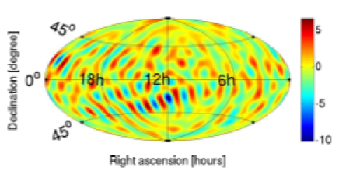
5) In the first panel of Figure 12 we plot an injection of a diffuse source clustered in the galactic plane. In the second panel we plot the clean sky map recovered from this injection using .
 |
 |
6) One way to test that an injection is recovered successfully and without bias is to plot the injected signal map minus the recovered clean map. To do this, we must take into account that the clean map was produced using SVD (see Section IV.2). That is, we need to compare the regularized extracted clean map with a ‘regularized’ version of the injected map:
| (83) |
Here is the Fisher matrix, is its regularized inverse, and is the injected map. In Figure 13 we plot for the galactic injection depicted in Figure 12.
|
|
 |
 |
 |
7) In the first panel of Figure 14 we plot an injection of a diffuse source clustered about generated using Planck simulator [49] and HEALPix [48]. In the mid-left panel we plot the regularized version of this injection, and in the top-right panel, a clean sky map using . In the mid-right panel we plot . The apparent quadrupole moment visible in the mid-left and top-right panels illustrates the relatively low sensitity to moments using the H1-L1 baseline.
 |
 |
 |
 |
 |
V.4 Sky maps - Multiple baselines
Figure 15 shows the clean sky maps for a diffuse source distributed along the galactic plane () and Figure 14 shows the clean sky maps for a diffuse source distributed along analyzed with single baselines (H1-L1), (H1-V1), and (L1-V1), and with the multi-baseline analysis (H1-L1-V1).
|
 |
 |
 |
|
VI SUMMARY
We have presented here a maximum-likelihood analysis method for estimating the angular distribution of power in an anisotropic stochastic gravitational-wave background. The basic idea was to cross-correlate data from a network of two or more gravitational-wave detectors, exploiting time-of-arrival differences and the diurnal modulation due to the Earth’s rotation. We derived maximum-likelihood estimators for the angular distribution of gravitational-wave power , decomposed with respect to any set of basis functions on the sky. We derived an expression for the beam pattern matrix and discussed its relationship to the covariance matrix of the maximum-likelihood estimators . We described how singular value decomposition can be used to regularize the inverse of , which was needed to remove the smearing effects of the beam pattern matrix on the measured (‘dirty’) sky maps . We also explained how the single-baseline (two-detector) cross-correlation analysis can be extended to a network of three or more detectors, thereby increasing our sensitivity to detecting a signal. In this paper, we focused attention on a decomposition with respect to a basis of spherical harmonics , for which the maximum-likelihood estimators represent the multipole moments of the gravitational-wave sky, and for which the standard isotropic and radiometer searches are recovered as special limiting cases. Finally, we illustrated all these general results by analysing simulated data containing injected stochastic gravitational-wave backgrounds having different angular power distributions.
Acknowledgements.
This work was supported by NSF grants: NSF-PHY0555842, NSF-PHY-0758172, NSF-PHY-0758036, and NSF-PHY-0757058. SM would like to acknowledge the Centre National d’Études Spatiales (France) for supporting part of the research. Part of the research described in this paper was carried out at the Jet Propulsion Laboratory, California Institute of Technology, under a contract with the National Aeronautics and Space Administration. This paper has been assigned LIGO document number LIGO-P0900083.Appendix A SPHERICAL HARMONICS
Our convention for the spherical harmonics follow [50]. Explicitly,
| (84) |
where are the associated Legendre functions defined by
| (85) | |||
| (86) |
The normalisation constants have been chosen so that
| (87) |
and
| (88) |
Note that
| (89) |
and
| (90) | |||||
| (91) | |||||
| (92) |
Expressions for the first few spherical harmonics (up to ) are given below:
| (93) |
| (94) |
| (95) |
| (96) |
| (97) |
| (98) |
| (99) |
| (100) |
| (101) |
Appendix B USEFUL IDENTITIES
The transformation property of the spherical harmonics (89) and (90) imply the following transformation property for the :
| (102) |
and
| (103) | |||||
| (104) |
Similarly, the requirement that is real implies
| (105) |
Finally, Eqs. (102), (103) and (104), together with the definition (47) and (48) imply
| (106) |
and
| (107) |
and
| (108) |
so is Hermitian.
Appendix C Detection statistic
In addition to estimating the individual components of an anisotropic stochastic background, it is also possible to construct a statistic that is optimal for detecting the presence of a background characterized by a particular set of (normalized) angular components and spectral shape . To show this, we note that in the presence of a signal, the components of the dirty map can be written in the form [32]
| (109) |
where and are as before, and is an additive noise term composed of cross-correlated detector noise and stochastic signal components. In the weak-signal approximation, the variance of the noise-noise cross-term, , is much greater than that of the signal-noise cross terms, and , so to a good approximation
| (110) |
Furthermore, when the detector noise is Gaussian and uncorrelated—an assumption that is well-approximated in practice—the are Gaussian-distributed with covariance matrix
| (111) |
To construct the detection statistic, we assume that the stochastic background has spectral shape and normalized angular components satisfying
| (112) |
The overall amplitude of the background is given by . Then the probability density function for the in the presence of such a background is given by the likelihood
| (113) |
By the Neyman-Pearson criterion, the optimal detection statistic is simply the maximum-likelihood estimator of [51]—that is,
| (114) |
The result, after a straightforward calculation is
| (115) |
which has the form of a standard matched-filter. Note that the detection statistic has zero mean and unit variance in the absence of a signal. In the presence of a signal whose parameters exactly match those of the signal model and , the expectation value of the statistic is
| (116) |
(The variance of the statistic is still unity in the weak-signal approximation.) In the special case of an isotropic background, , which is the signal-to-noise ratio for the standard isotropic search.
References
- [1] http://www.ligo.caltech.edu/.
- [2] B. C. Barish and R. Weiss, Physics Today 52, 44 (1999).
- [3] B. P. Abbott et al. (The LIGO Scientifc Collaboration) (2009), eprint http://arxiv.org/pdf/0711.3041v2.
- [4] B. P. Abbott et al., Nucl. Instr. Meth. A 517, 154 (2004a).
- [5] http://www.virgo.infn.it/.
- [6] C. Bradaschia et al., Nuclear Instruements and Methods in Physics Research A 289, 518 (1990).
- [7] http://www.geo600.uni-hannover.de/.
- [8] B. Wilke et al., Classical and Quantum Gravity 21, S417 (2004).
- [9] B. Abbott et al., Physical Review D 77, 062002 (2008a), eprint arXiv:0704.3368.
- [10] B. Abbott et al., Physical Review D 79, 122001 (2009a), eprint arXiv:0901.0302.
- [11] B. Abbott et al. (The LIGO Scientific Collaboration) (2009), arxiv:0905.1654.
- [12] LIGO Scientific Collaboration (2009), arxiv:0905.3710.
- [13] B. Abbott et al., to appear in PRL (2008b), eprint arXiv:0808.2050.
- [14] B. Abbott et al., Physical Review D 76, 062003 (2007a), eprint astro-ph/0703419.
- [15] B. Abbott et al., Physical Review D 76, 042001 (2007b), eprint gr-qc/0702039.
- [16] B. Abbott et al., Physical Review D 77, 022001 (2008c), eprint arXiv:0708.3818.
- [17] B. Abbott et al., Astrophysical Journal 681, 1419 (2008d), eprint arXiv:0711.1163.
- [18] B. Abbott et al., Physical Review D 77, 0620004 (2008e), eprint arXiv:0709.0766.
- [19] B. Abbott et al., Class. Quantum Gravity 24, 5343 (2007c), eprint arXiv:0704.0943.
- [20] B. Abbott et al., Class. Quant. Grav. 23, S29 (2006), eprint gr-qc/0511146.
- [21] B. Abbott et al., Physical Review D 76, 082003 (2007d), eprint astro-ph/0703234.
- [22] 07B. Abbott et al. LIGO-ALLEGRO B. Abbott et al. (LIGO Scientific Collaboration and ALLEGRO Collaboration, PRD 76, 022001 (2007).
- [23] B. Abbott et al., Astrophysical Journal 659, 918 (2007e), eprint astro-ph/0608606.
- [24] M. Maggiore, Physics Reports 331, 283 (2000).
- [25] E. W. Kolb and M. Turner, The Early Universe (Addison Wesley, 1990).
- [26] B. Abbott et al., Nature 460, 990 (2009b).
- [27] B. Abbott et al., ApJ Lett 683, 45 (2008f), eprint arXiv:0805.4758.
- [28] C. Palomba, Astronomy & Astrophysics 354, 163 (2000).
- [29] T. L. Smith, E. Pierpaoli, and M. Kamionkowski, PRL 97, 021301 (2006).
- [30] B. Abbott et al., Physical Review D 69, 122004 (2004b), eprint gr-qc/0312088.
- [31] B. Abbott et al., Physical Review Letters 95, 221101 (2005), eprint astro-ph/0507254.
- [32] S. Mitra, S. Dhurandhar, T. Souradeep, A. Lazzarini, V. Mandic, S. Bose, and S. Ballmer, Physical Review D 77, 1550 (2008).
- [33] N. J. Cornish, CQG 18, 4277 (2001).
- [34] K. Cannon, PRD 75, 123003 (2007).
- [35] T. Regimbau and V. Mandic, CQG 25, 184018 (2008).
- [36] L. A. Boyle and P. J. Steinhardt, PRD 77, 063504 (2008).
- [37] B. Allen and J. Romano, Physical Review D 59, 102001 (1999).
- [38] B. Allen and A. Ottewill, Physical Review D 56, 545 (1997).
- [39] L. S. Finn, S. L. Shane, and J. D. Romano, PRD 79, 062003 (2009).
- [40] N. Christensen, Physical Review D 46, 5250 (1992).
- [41] É. É. Flanagan, Physical Review D 48, 2389 (1993).
- [42] G. Hinshaw et al., In press (2006), eprint astro-ph/0603451.
- [43] S. W. Ballmer, Classical and Quantum Gravity 23, S179 (2006).
- [44] D. S. Sivia, Data analysis: a Bayesian tutorial (Oxford University Press, 1996).
- [45] J. Skilling, Bayesian Analysis 1, 833 (2006).
- [46] B. P. Abbott et al., Rep. .Prog. Phys. 72, 076901 (2009c), eprint arxiv/0711.3041.
- [47] F. Acernesea et al., Optics and Lasers in Engineering 45, 478 (2007).
- [48] K. M. Górski, E. Hivon, A. J. Banday, B. D. Wandelt, F. K. Hansen, M. Reinecke, and M. Bartelmann, Astrophysical Journal 622, 759 (2005).
- [49] Planck simulator, http://www.g-vo.org/planck/.
- [50] J. D. Jackson, Classical Electrodynamics (Wiley, 1975).
- [51] C. W. Helstrom, Statistical Theory of Signal Detection (Pergamon, London, 1968).