Excitations of the $\nu=5/2$ Fractional Quantum Hall State and the Generalized Composite Fermion Picture

The energy spectrum of a pure two-dimensional electron gas in a strong perpendicular magnetic field is completely determined by the Coulomb interactions, making it the paradigm for all “strongly interacting” systems, (for which standard many body perturbation theory is inapplicable). Jain’s composite Fermion (CF) picture [1, 2] has emerged as a comprehensive approach to understanding the most prominent incompressible states of the lowest Landau level (LL0). The original CF picture made use of a mean-field Chern-Simons (CS) gauge field theory. The CFs are electrons that have an even number Chern-Simons (CS) fluxes attached. The remarkable feature of this model is that it maps complicated FQH states with filling factor $\nu$ into simpler and better understood states of CFs with effective filling factor $\nu^{\ast}$. A good example is provided the well-known series of Laughlin-Jain states [3, 4] occurring at filling factors $\nu=\nu^{\ast}/(2p\nu\pm 1)$ where $\nu^{\ast}$ and $p$ are integers. The mean-field approach deals with two scales of energy: the cyclotron energy $\hbar\omega_{c}$ and the Coulomb interaction scale $e^{2}/\lambda$ where the cyclotron frequency is $\omega_{c}=(eB)/(mc)$ and the magnetic length is $\lambda=\sqrt{(\hbar c)/(eB)}$. In numerical studies and in some realistic systems, the cyclotron energy is much larger than the average Coulomb energy; thus the former scale is irrelevant. The low lying energy states are completely determined by Coulomb interactions. Adiabatic addition of flux [5] introduces Laughlin correlations without the need of a new mean-field cyclotron energy scale. Generalization of the CF picture to a plasma containing more than one type of particle was first introduced by Wójs et al. [6]. It was used to predict the low lying band of states of systems containing both electrons and valence band holes. In this case the the constituents (electrons and negatively charged excitons) have the same charge. In this paper we propose a new generalization of CF model to include multi-component plasmas in which particles with different charges are involved. We use this model to suggest an explanation of the low-lying bands of states of the $\nu=5/2$ FQH states.

The $\nu=5/2$ state has generated considerable recent interest as the result of the suggestion that its elementary excitations can be non-Abelian quasiparticles. Such excitations occur when the three particle pseudopotential $V(\mathcal{R}_{3})$ of Greiter et al.[7], which forbids the formation of compact three particle clusters, is used to describe the interactions of electrons in the first excited Landau level (LL1). Our simple generalized CF picture is used to interpret the ground state and low lying bands of excitations of electrons in LL1 interacting through the standard Coulomb pseudopotential appropriate for such electrons confined to a very narrow quantum well. New experimental results of Choi at al. [8] have been used to interpreted incompressible states in terms of formation of pairs (with $\ell_{\rm{P}}=2\ell-1$) or large clusters at filling factors $\nu_{1}=\nu-2$ of LL1 with $2/3\geq\nu_{1}\geq 1/3$. The most prominent IQL state occurs at $2\ell=2N-3$ (or at $2\ell=2N+1$). Here we present numerical results for the energy spectrum for $N=8,10,12$ and $14$. We demonstrate that in addition to the $L=0$ ground states, the two lowest band of excitations can be interpreted using our simple generalization of Jain’s CF picture to a two component plasma of Fermion pairs (FPs) and unpaired electrons.

The paper is organized as follows. The next section is dedicated to the solution of a two particle system in a magnetic field. The third section discusses CS gauge transformation and adiabatic addition of CS flux. In the fourth section, we present the generalized CF model and its application to the $\nu=5/2$ FQH state. We draw conclusions in the last section.

A two particle system is the simplest system that can be used to understand the physics of introducing the CS flux. The two particles have masses $m_{1}$ and $m_{2}$ and charges $q_{1}$ and $q_{2}$ and they are moving in the $x-y$ plane. A dc uniform magnetic field $\vec{B}=B\hat{z}$ is applied perpendicular to the plane. We work in the symmetric gauge where the vector potential is $\vec{A}=\frac{1}{2}Br\hat{\phi}$, where $\hat{\phi}$ is the unit vector in the direction of increasing the angular coordinate $\phi$ . The Hamiltonian contains the kinetic terms and the Coulomb term.

The Hamiltonian can be separated into the center of mass (CM), relative (R) part, and a part describing the interaction between the CM and R motions (I).

Here relative coordinate and momentum are $\vec{r}=\vec{r}_{1}-\vec{r}_{2}$ and $\vec{p}=\frac{1}{2}(\vec{p}_{1}-\vec{p}_{2})$, respectively. The reduced mass and charge are $\mu=(m_{1}m_{2})/(m_{1}+m_{2})$ and $q=(q_{1}m_{2}^{2}+q_{2}m_{1}^{2})/(m_{1}+m_{2})^{2}$. $R=\frac{1}{2}(\vec{r}_{1}+\vec{r}_{2})$ and $\vec{P}=\vec{p}_{1}+\vec{p}_{2}$ represent the CM coordinate and momentum. Also $\bar{q}=(q_{1}m_{2}+q_{1}m_{2})/(m_{1}+m_{2})$ and $\tilde{q}=(q_{1}m_{2}-q_{2}m_{1})/(m_{1}+m_{2})$. Throughout this paper we consider that the particles have the same charge to mass ratio (specific charge) $q_{1}/m_{1}=q_{2}/m_{2}$, and as a consequence the $\tilde{q}=0$ and the CM and R motions decouple.

The solution of Schrödinger equation of the relative motion can be written as $\Psi_{nm}=e^{im\phi}u_{nm}(r)$. Exchanging the particles corresponds to replacing $\phi$ by $\phi+\pi$. Therefore, if particles are Fermions (Bosons), $m$ must be odd (even). The radial function $u_{nm}(r)$ satisfies the following equation

where $\rho=r/\lambda_{r}$, $\lambda_{r}=[(\hbar c)/(qB)]^{1/2}$ is the magnetic length for the relative motion. The parameter $\eta_{0}$ characterizes the strength of Coulomb interaction with respect to cyclotron energy. $\eta_{0}=(q^{2}/\lambda_{r})/(\hbar\omega_{cr})$ and $\omega_{cr}=(qB)/(mc)$ is the cyclotron frequency of the relative motion. The eigenvalues of $H_{R}$ are $E_{mn}=(\hbar\omega_{cr}/2)\epsilon_{nm}$. $n=0,1,2,\cdots$ is a non-negative integer number, while $m$ is an integer less than or equal to $n$.

In the absence of the electron-electron term the solutions is well-known

The lowest Landau level wavefunction has its maximum value at $\rho=\sqrt{2|m|}$. The eigenvalues are $\epsilon_{nm}=2n+1+m+|m|$.

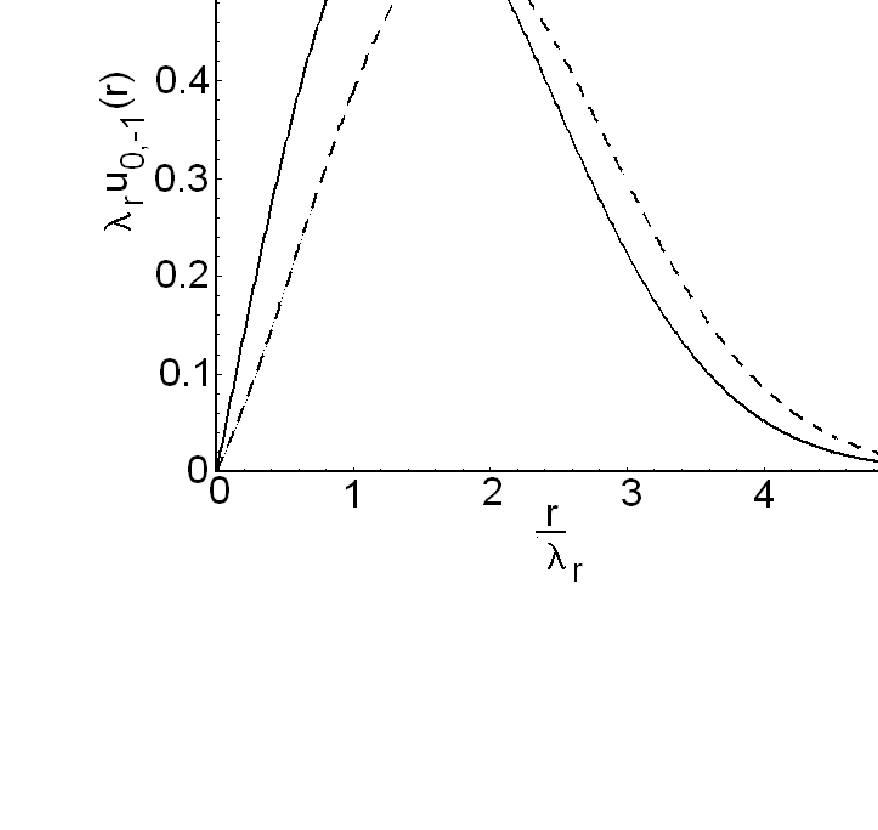
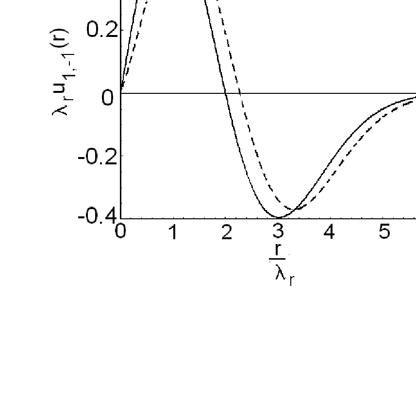
If the Coulomb interaction is taken into account, the degeneracy of the Landau levels is lifted. States with small values of $m$ have the largest increase in energy. In Fig. 1, we plot the energy levels vs. the relative strength of Coulomb interaction for a system of 2 electrons. Coulomb interaction does not alter fundamentally the shape of the wavefunction at least for small values of $(e^{2}/\lambda_{r})/(\hbar\omega_{cr})$, preserving the small and large distance behavior. The radial part of the wavefunction for $\eta_{r}=0.25$ together with the corresponding one for noninteracting particles are plotted in Fig. 2 for the same two-electron system.

The CF picture [1, 2] results from the introduction of C-S fluxes. The vector potential $\vec{a}(\vec{r})$ that produces a flux of $\Phi=\alpha\Phi_{0}=\alpha hc/e$ is

where $\rho(\vec{r})=\Psi^{\dagger}(\vec{r})\Psi(\vec{r})$ is the density operator. The magnetic field resulting from the CS vector potential is given by $\vec{b}(\vec{r})=\Phi\sum_{i}\delta(\vec{r}-\vec{r}_{i})\hat{z}$ where $\vec{r}_{i}$ is the position of the $i^{\rm{th}}$ electron.

A charged particle is moving on a circular path in $x-y$ having the wavefunction $\Psi(\vec{r})=e^{im\phi}u_{m}(r)$. When the flux tube is added via a gauge transformation, the eigenfunction is changed to

Considering $\vec{a}(\vec{r})=\hat{\phi}\Phi/(2\pi r)$, the new wavefunction is $\overline{\Psi}(\vec{r})=\exp(i(m-\alpha)\phi)u_{m}(r)$. The CS flux does not influence the radial wavefunction, but it introduces a phase of $-i\alpha\phi$. For relative motion of the pair of charges, an odd integer $\alpha$ generates the famous change of statistics from bosons to fermions and viceversa. Introducing the CS flux, makes the many-body Schrödinger equation extremely complicated. A simplification occurs when the mean-field approximation is made by replacing the density operator by its ground state average density $n=<\Psi^{\dagger}\Psi>$ in the expression of the CS vector potential. The particles move in an effective magnetic field $B^{*}=B+\alpha\phi_{0}n$ and the mean-filed Coulomb interaction vanishes. The mean-field approximation introduces an effective cyclotron energy scale $\hbar\omega_{c}^{\ast}=(\hbar qB^{\ast})/(\mu c)$, which is irrelevant since $q^{2}/\lambda_{r}<<\hbar\omega_{c}^{\ast}$.

Instead of making a gauge transformation we can introduce the CS fluxes adiabatically [5]. We start with initial electron pair state and slowly increase the value of CS flux. Such technique leaves the phase of the wavefunction unchanged, but the radial wavefunction is modified $u_{m}(r)\rightarrow u_{m+\alpha}(r)$ (in the absence of Coulomb interaction).

In the case of the system made of two particles with different charges, the fluxes attached to the two particles are increased from zero to $\alpha\phi_{0}$ and $\beta\phi_{0}$ respectively. The Hamiltonian is

where $a(\vec{r})=\hat{\phi}(\phi_{0}/2\pi r)$. We suppose again that the particles have the same specific charges. The Hamiltonian can be decomposed into a CM part, an R part, and interaction between the CM and R motions.

where $q_{\alpha}=q_{1}\alpha-q_{2}\beta$ The CM and relative motions decouple completely if $q_{\alpha}=0$, i.e. $q_{1}\alpha=q_{2}\beta$. This condition can be used to develop the generalized CF picture for a plasma containing particles with different charges. The relative motion Hamiltonian is very similar to Eq. 3. The effective magnetic field is modified by the CS flux. The new wavefunction will not change its phase, but the orbital part is modified.

We introduce a generalized CF picture for a multicomponent plasma. We think of every species of charged particle present in the plasma as a having different color (red, blue, etc.). We attach to each particle a flux tube carrying an integral number of different flux quanta of different colors. Each charge will see only the flux tubes having the same color, and no particles will see its own flux. For example a “red” charge will see the red flux tubes attached to all other particles. The correlations between the particles having the same color is identical to the one introduced in the original CF picture. The generalized CF model also introduces the correlations between different type of particles. We need to obtain the same correlations when “blue” charges interacts with “blue” fluxes on “red” charges as when “red” charges interact with “red” fluxes attached to blue charges. Adding $pq_{red}/e$ “blue” fluxes to the a “red” charge causes the “blue” charge to have exactly the same blue-red correlations as adding $pq_{blue}/e$ “red” fluxes to blue charge. The CS charge times the CS flux must be the same.

In this section, we use the Haldane’s spherical geometry [9], which maps the infinite planar surface onto a spherical one, magnetic field being produced by a monopole placed in the center of the sphere. The monopole strength is $2Q\Phi_{0}$ (where $2Q$ is an integer) gives rise to a magnetic field $B=2Q\Phi_{0}/(4\pi R^{2})$ which is perpendicular to the spherical surface. The single particle eigenstates are called monopole harmonics and denoted by $|Q,\ell,m>$[10, 11]. They are eigenfunctions of the square of the angular momentum operator $\hat{\ell}^{2}$ and its $z-$projection $\hat{\ell}_{z}$ with eigenvalues $\ell(\ell+1)$ and $m$ respectively, and $|m|\leq\ell$. Landau levels are replaced by angular momentum shells $\ell=Q+n$, where $n$ plays the role of the LL index. The energy of the state $|Q,\ell,m>$ is $E_{\ell}=(\hbar\omega_{C}/2Q)[\ell(\ell+1)-Q^{2}]$. In order to obtain the energy spectrum of an $N-$particle system, the Coulomb interaction $e^{2}/r_{ij}$, is diagonalized in the non-interacting basis set.

In this geometry, the effective monopole strength seen by CFs of “color” $a$ will be

with $q_{a}m_{ab}=q_{b}m_{ba}$.

This model is applied to understand the lowest bands of states in the case of $\nu=5/2$ state. It is clear that the correlations and the elementary excitations are better understood for LL0 than for LL1 and higher Landau levels. The Coulomb interaction is described using the pseudopotentials $V(\mathcal{R})$, where $\mathcal{R}$ is the relative angular momentum $\mathcal{R}=2\ell-L^{\prime}$, $L^{\prime}$ being the pair angular momentum. It is well-known that Laughlin correlations (the avoidance of pair states with small values of $\mathcal{R}$) occur only when the pseudopotential $V_{n}(\mathcal{R})$ describing the interaction energy of a electron pair with angular momentum $L^{\prime}=2\ell-\mathcal{R}$ in LLn is “superharmonic”, i.e. rises with increasing $L^{\prime}$ faster than $L^{\prime}(L^{\prime}+1)$ as the avoided value of $L^{\prime}$ is approached [12, 13, 14]. A pseudopotential that is not “superharmonic” does not induce Laughlin correlations [15] and instead results in formation of pairs. In LL0 the pseudopotential is superharmonic for all values of $\mathcal{R}$. The CF picture applied for electrons in LL0, introduces $\ell^{\ast}=|\ell-p(N-1)|$, where $p$ is an integer and explains that the lowest band of states will contain the minimum number of QP excitations required by the values of $N$ and $2\ell$ [16] The QHs reside in the angular momentum shell $\ell_{\rm{QH}}=\ell^{\ast}$; the QEs are in the shell $\ell_{\rm{QE}}=\ell_{\rm{QH}}+1$.

In LL1, the pseudopotential is only “weakly” superharmonic [17, 18] for $R=1$ and as a consequence it does not support Laughlin correlations at $1/3\leq\nu_{1}\leq 2/3$[19]. The correlations can be described in terms of the formation of $N_{\rm{P}}=N/2$ pairs[19] when $N$ is even. The electrons tend to form pairs with $\ell_{\rm{P}}=2\ell-1$. To avoid violating the exclusion principle, we can’t allow Fermion pairs (FPs) to be too close to one another. We do this by restricting the angular momentum of two pairs to values less than or equal to [20, 21, 22, 23]

implying that the FP filling factor satisfies the relation $\nu_{\rm{FP}}^{-1}=4\nu_{1}^{-1}-3$. The factor of 4 is a reflection of $N_{\rm{P}}$ being half of $N$ and the LL degeneracy $g_{\rm{P}}$ of the pairs being twice $g$ for electrons. Correlations are introduced through a standard CF transformation applied to FPs:

Selecting $2p_{\rm{P}}=4$ results in $2\ell_{\rm{FP}}^{*}+1=N_{\rm{P}}$ and pairs forming a $L=0$ incompressible quantum liquid (IQL) ground state. This occurs if the number of electrons and the angular momentum shell satisfy the relation $2\ell=2N-3$ (or the electron-hole conjugate $2\ell=2N+1$). These IQL states are marked by circles in Fig. 3.

In order to understand the lowest bands of states we will assume two types of elementary excitations. The first type will consists of an empty FP state in the lowest FP level [a quasi-hole FP (QHFP) with angular momentum $\ell_{\rm{FP}}^{\ast}$] plus one filled FP state in the first excited FP level [a quasiparticle FP (QPFP) with angular momentum $\ell_{\rm{FP}}^{\ast}+1$]. Since $2\ell_{\rm{FP}}^{\ast}=(N_{\rm{P}}-1)$, this process give rise to a “magnetoroton” state of a QHFP with $\ell_{\rm{QHFP}}=(N_{\rm{P}}-1)/2$ and a QPFP with $\ell_{\rm{QPFP}}=(N_{\rm{P}}+1)/2$. The resulting“magnetoroton” band has $L=1\oplus 2\oplus\ldots\oplus N_{\rm{P}}$. This band is marked by squares in Fig. 3. Up to an overall constants this band represents the interaction pseudopotential of a QHFP and a QPFP as a function of the total angular momentum. Unfortunately the width of the band is not small compared to the minimum gap required to produce a magnetoroton of FPs, so it is not as useful as the QE and QH pseudopotential obtained from Laughlin correlated states in LL0 which contain a pair of QEs or a pair of QHs [16].

Another possible band of low lying excitations could result from breaking one of the CF pairs into two constituent unpaired electrons, each with charge $-e$ and angular momentum $\ell$. We propose to treat the system of $N_{\rm{P}}^{\prime}=N_{\rm{P}}-1$ FPs and the $N_{e}=2$ unpaired electrons by our generalized CF picture. Let the $2\ell_{\rm{FP}}^{\prime}=2\ell_{\rm{P}}-3(N_{\rm{P}}^{\prime}-1)$. Then the following equations describe correlations of the $N_{\rm{P}}^{\prime}$ FPs and $N_{e}=2$ unpaired electrons:

Eq. 16 tells us that the effective angular momentum of one FP is decreased from $\ell_{\rm{FP}}$ by $p_{\rm{P}}$ times the number of other FPs and by $\gamma$ times the number of unpaired electrons. Eq. 17 tells us that the effective angular momentum of one unpaired electron is decreased by $p_{e}$ times the number of other unpaired electrons and by $\gamma/2$ times the number of CF pairs. Note that $2p_{\rm{FP}}$ and $2p_{e}$ are even, and that $\gamma$ can be odd or even. Equations 16 and 17 define the generalized CF picture in which different types of Fermions, distinguishable from one another, experience correlations which leave them as Fermions (since $2p$ is even) and give the same correlations between members of two different species since the product of CS charge and the CS flux added are the same (i.e $-e\cdot 2\gamma=-2e\cdot\gamma$).

When using $p_{\rm{P}}=2$, $p_{e}=1$, $\gamma=2$, $N_{\rm{P}}^{\prime}=N_{\rm{P}}-1$ and $N_{e}=2$, and $2\ell_{\rm{FP}}^{\prime}=2\ell_{\rm{P}}-3(N_{\rm{P}}^{\prime}-1)$, eq. 16 give the FPs effective angular momentum as $\ell_{\rm{FP}}^{\prime\ast}=N_{\rm{P}}-2$ and the FPs will form an IQL $L=0$ state. The 2 electrons become CFs occupying the level $2\ell_{e}^{\ast}=N-3$. They generate the “broken pair” band of states at $L=0\oplus 2\oplus\cdots\oplus N-4$. This band of states is represented by triangles in Fig. 3.

Some of these states were discussed by Greiter et al. [24, 7] but not in terms of a generalized CF picture capable of predicting the allowed values of $L$ in the lowest band of energy levels.

We developed a generalized CF model in which a plasma contains particles with different charges. The adiabatic introduction of CS fluxes was used. It is worth noting that for the generalized CF picture the correlations between a pair of particles can be thought of as resulting from adiabatic addition of fictitious CS flux quanta to one particle that is sensed by fictitious charge on the other. We applied our model to the system with $\nu=5/2$ filling factor. Our interpretation is an attempt to understand some of the low lying excitations of the $\nu_{1}=1/2$ state in a simple CF type picture. The numerical data confirm our model. Our results do not contain degenerate QP states that give rise to non-Abelian statistics. Further studies with realistic electron pseudopotentials should be undertaken to see if non-Abelian quasiparticles appearing at values of $2\ell$ slightly different than $2N-3$ are only an artifact of the Greiter, Wen and Wilczek model interaction.

References

- [1] J. K. Jain, Phys. Rev. Lett. 63, 199 (1989a).
- [2] J. K. Jain, Phys. Rev. B 41, 7653 (1990).
- [3] R. B. Laughlin, Phys. Rev. Lett. 50, 1395 (1983).
- [4] J. K. Jain, Phys. Rev. B 40, 8079 (1989b).
- [5] J. J. Quinn and J. J. Quinn, Phys. Rev. B 68, 153310 (2003).
- [6] A. Wójs, I. Szlufarska, K.-S. Yi, and J. J. Quinn, Phys. Rev. B 60, R11273 (1999).
- [7] M. Greiter, X.-G. Wen, and F. Wilczek, Nucl. Phys. B 374, 567 (1992).
- [8] H. C. Choi, W. Kang, S. Das Sarma, L. N. Pfeiffer, and K. W. West, Phys. Rev. B 77, 081301(R) (2008).
- [9] F. D. M. Haldane, Phys. Rev. Lett. 51, 605 (1983).
- [10] T. T. Wu and C. N. Yang, Nucl. Phys. B 107, 365 (1976).
- [11] T. T. Wu and C. N. Yang, Phys. Rev. D 16, 1018 (1977).
- [12] A. Wójs and J. J. Quinn, Solid State Commun. 108, 493 (1998).
- [13] A. Wójs and J. J. Quinn, Solid State Commun. 110, 45 (1999).
- [14] J. J. Quinn and A. Wójs, Physica E 6, 1 (2000).
- [15] P. Sitko, K.-S. Yi, and J. J. Quinn, Phys. Rev. B 56, 12417 (1997).
- [16] X. M. Chen and J. J. Quinn, Phys. Rev. B 47, 3999 (1993).
- [17] A. Wójs, Phys. Rev. B 63, 125312 (2001).
- [18] A. Wójs and J. J. Quinn, Phys. Rev. B 71, 045324 (2005).
- [19] G. E. Simion and J. J. Quinn, Physica E 41 (2008).
- [20] J. J. Quinn, A. Wójs, and K.-S. Yi, Phys. Lett. A 318, 152 (2003).
- [21] A. Wójs, D. Wodziński, and J. J. Quinn, Phys. Rev. B 71, 245331 (2005).
- [22] A. Wójs, D. Wodziński, and J. J. Quinn, Phys. Rev. B 74, 035315 (2006).
- [23] J. J. Quinn and J. J. Quinn, Solid State Commun. 140, 52 (2006).
- [24] M. Greiter, X.-G. Wen, and F. Wilczek, Phys. Rev. Lett. 66, 3205 (1991).