Calculation of the Raman $G$ peak intensity in monolayer graphene: role of Ward identities

In the past decades, Raman spectroscopy [1] techniques were successfully applied to carbon compounds, such as graphite [2] and carbon nanotubes [3]. Upon the discovery of graphene [4], Raman spectroscopy has proven to be a powerful and non-destructive tool to identify the number of layers, doping, disorder, strain, and to characterize the phonons and electron-phonon coupling [5, 6, 7, 8, 9, 10, 11].

The most robust feature in the Raman spectra of all conjugate carbon compounds is the so-called $G$ peak, corresponding to the in-plane bond-stretching optical vibration of $sp^{2}$-hybridized carbon atoms. In graphene this vibration has the $E_{2g}$ symmetry, it is doubly degenerate, and its frequency $\omega_{\mathrm{ph}}\approx{1580}\>\mbox{cm}^{-1}$. While the $G$ peak frequency is sensitive to external factors, such as doping level [6, 7, 8] or strain [12, 10, 11], its total frequency-integrated intensity $I_{G}$ is often assumed to remain constant under the change of many external parameters, depending only on the excitation frequency. Thanks to this robustness, $I_{G}$ is often used as a reference to which intensities of other peaks are compared [13, 14, 15], since measurement of absolute peak intensities represents a hard experimental task (the first use of $I_{G}$ as a reference for other Raman peak intensities in graphite probably dates back to 1970 [16]).

Given this popular role of $I_{G}$ as a reference, it is clear that having at hand a theoretical expression of the absolute intensity in terms of the basic parameters of the material (such as the electronic dispersion, the electron-phonon coupling, etc.), would be useful. Nevertheless, to the best of the author’s knowledge, no such expression is available at present. $I_{G}$ was discussed in a recent paper by the author [17], where the conclusion was reached that even in the limit when the excitation frequency $\omega_{\mathrm{in}}$ is small compared to the energy scale $t_{0}$ characterizing the electronic dispersion (several eV), the intensity $I_{G}$ is contributed by the whole conduction and valence bands, not just by low-energy states in the vicinities of the Dirac points. As will be shown below, this conclusion is wrong, since Ref. [17] missed strong cancellations occurring as a consequence of a Ward identity. This affects the dependence of $I_{G}$ on $\omega_{\mathrm{in}}$.

In the present work $I_{G}$ is calculated for a clean graphene monolayer suspended in vacuum. When $\omega_{\mathrm{in}}\ll{t}_{0}$, the intensity is indeed determined only by electronic states with energies $\sim\omega_{\mathrm{in}}$, not the whole conduction and valence bands (however, these energies do not have to be close to $\omega_{\mathrm{in}}/2$). In this limit $I_{G}$ can be expressed in terms of a few parameters, characterizing these low-energy states. As correctly mentioned in Ref. [17], trigonal warping of the electronic bands and the anisotropy of the electron-hole coupling turn out to be crucial for the $G$ peak. In the limit $\omega_{\mathrm{ph}}\ll\omega_{\mathrm{in}}\ll{t}_{0}$ the frequency dependence is $I_{G}\propto\omega_{\mathrm{in}}^{2}$. At higher frequencies, the calculation is performed using the nearest-neighbor tight-binding model. The main feature found is a strong enhancement of $I_{G}$ when the frequency matches the energy of electron-hole separation at the $M$ point of the electronic first Brillouin zone, where a van Hove singularity in the electronic density of states occurs.

The Bloch form of the electronic wave function in the tight-binding model is

where $\psi_{\mathrm{a}}(\mathbf{r})$ is the atomic wave function localized near the origin, $\alpha=A,B$ labels the sublattices, and the two-dimensional integer vector $\mathbf{n}$ labels the unit cells, each containing two atoms from the two sublattices. The wave vector $\mathbf{k}$ runs over the first Brillouin zone. The Bloch amplitudes $\mathcal{U}_{\alpha\mathbf{k}}$ satisfy the Shrödinger equation (we neglect the non-orthogonality of the atomic orbitals)

where the Hamiltonian matrix is given by

Suppose that all atoms belonging to the sublattice $\alpha$ are displaced by $\mathbf{u}_{\alpha}$, and $\mathbf{u}_{A}=-\mathbf{u}_{B}$. Such a uniform displacement corresponds to optical phonons with the wave vector $\mathbf{q}=0$. These are the phonons responsible for the $G$ peak, as fixed by the momentum conservation (the wave vectors of both incident and scattered photons are negligibly small). In the tight-binding model the mechanism of the electron-phonon coupling is the change of the nearest-neighbor electronic matrix element $t_{0}$ due to the change in the bond length $a$, $\partial{t}_{0}/\partial{a}\approx-6\>\mbox{eV}/\mbox{\AA}$. Then, to linear order in the atomic displacements, the electron-phonon interaction Hamiltonian is given by

The electromagnetic field of the incident and scattered light is described by the vector potential $\mathbf{A}$. The Hamiltonian describing interaction of the electrons with the field can be obtained by the Peierls substitution $\mathbf{k}\to\mathbf{k}-(e/c)\mathbf{A}$ in the electronic Hamiltonian. Since we are interested in a two-photon process, we should expand the Hamiltonian to the second order in $\mathbf{A}$:

Here $i,j,l=x,y$ label the in-plane Cartesian components, and the summation over repeated indices is assumed. Note that for the description of resonant multiphoton processes it is sufficient to keep $\hat{H}_{\mathbf{k}}^{(1)}$ term only, as it was done in [17], since the contribution of other terms is (i) off-resonant and (ii) smaller by a factor $\sim\omega_{\mathrm{in}}/t_{0}$. However, for the one-phonon process studied here the contributions from all terms turn out to be of the same order; in fact, they almost cancel each other.

To calculate the Raman scattering probability, we follow the general steps of Ref. [17]: pass to the second quantization, calculate the scattering matrix element, and substitute it into the Fermi Golden Rule. The zero-temperature electronic Green’s function is a $2\times{2}$ matrix,

Upon quantization of the phonon field the atomic displacements corresponding to the optical phonons are expressed in terms of the phonon creation and annihilation operators $\hat{b}_{\mathbf{q},\mu}^{\dagger},\hat{b}_{\mathbf{q},\mu}$ as

Here $\mu=x,y$ labels the two degenerate phonon modes, $\mathbf{e}^{(\mu)}$ is the unit vector in the corresponding direction, $M$ is the mass of the carbon atom, $N$ is the total number of the carbon atoms in the crystal, and “h.c.” stands for the hermitian conjugate. A small finite wave vector $\mathbf{q}$ has to be introduced in order to treat the in-plane momentum conservation properly; only the $\mathbf{q}=0$ modes will contribute to the final result. The transverse electromagnetic field is quantized inside the large volume $L_{x}L_{y}L_{z}$ in the Coulomb gauge:

Here $\mathbf{Q}$ is the three-dimensional wave vector, $\ell=1,2$ labels the two transverse polarizations along the two unit vectors $\mathbf{e}^{(\mathbf{Q},\ell)}\perp\mathbf{Q}$.

The probability for an incident photon with the polarization $\mathbf{e}^{\mathrm{in}}$ and frequency $\omega_{\mathrm{in}}$ to be scattered into an element of the solid angle $do_{\mathrm{out}}$ with the polarization $\mathbf{e}^{\mathrm{out}}$, and with the frequency $\omega_{\mathrm{out}}=\omega_{\mathrm{in}}-\omega_{\mathrm{ph}}$ fixed by the energy conservation, is given by

Here $\mathcal{M}^{ijl}$ is the transition matrix element (the factor of 2 explicitly takes care of the two spin projections of the electron). It is given by the sum of the following contributions:

The factor $\rme^{{\rmi}\epsilon{0}^{+}}$ prescribes closing of the $\epsilon$-integration contour in the upper half-plane. In fact, it is important only for the last term, Eq. (3if) which corresponds to the sum over the filled valence band. Upon integration over $\epsilon$, Eq. (3h) reduces to the standard perturbation theory expression for the Raman amplitude as the sum over intermediate states. Each intermediate state contains an electron with the wave vector $\mathbf{k}$ in the conduction band and a hole in the valence band with the wave vector $-\mathbf{k}$. The $\mathbf{k}$ integration is performed over the first Brillouin zone. The six terms given by Eqs. (3ia)–(3if) can be represented pictorially by the diagrams shown in Fig. 2. In fact, $\mathcal{D}_{1\mathbf{k}}=\bar{\mathcal{D}}_{1\mathbf{k}}$ because the Green’s function and all the vertex matrices satisfy $\hat{G}_{\mathbf{k}}^{T}(\epsilon)=\hat{\sigma}_{x}\hat{G}_{\mathbf{k}}(\epsilon)\hat{\sigma}_{x}$ and $\hat{G}_{\mathbf{k}}(-\epsilon)=-\hat{\sigma}_{z}\hat{G}_{\mathbf{k}}(\epsilon)\hat{\sigma}_{z}$ (the $T$ superscript denotes the matrix transpose, and $\hat{\sigma}_{x,z}$ are the Pauli matrices).

If one integrates each of the terms in Eqs. (3ia)–(3if) separately, the main contribution to the $\mathbf{k}$-integral comes from the “bulk” of the first Brillouin zone, rather than the vicinities of the Dirac points (as it was pointed out in Ref. [17]). Let us formally consider, however, the whole expression for $\mathcal{M}^{ijl}$ at $\omega_{\mathrm{in}}=\omega_{\mathrm{out}}=0$. Then the sum of the terms (3ia)–(3if) is a total derivative, $\partial^{2}[\hat{F}_{\mathbf{k}}^{l}\hat{G}_{\mathbf{k}}(\epsilon)]/(\partial{k}_{i}\partial{k}_{j})$. Thus, the $\mathbf{k}$-integral vanishes, i. e., at $\omega_{\mathrm{in}}=\omega_{\mathrm{out}}=0$ all terms contributing to the matrix element, cancel. This cancellation is far more general than the tight-binding model, used here. Indeed, consider linear response of the electronic current $\mathbf{j}$ to a static homogeneous vector potential $\mathbf{A}$. The corresponding response function $\chi_{ij}$ must vanish, since an observable (current) cannot respond to a pure gauge¹¹ 1 Strictly speaking, it is the limit $\lim_{\mathbf{q}\to{0}}\lim_{\omega\to{0}}\chi_{ij}(\mathbf{q},\omega)$ which vanishes, while the calculation done in this work corresponds to the opposite order of limits. The two limits commute for undoped graphene, when the Fermi surface has zero length. At finite doping, the contribution of the filled valence band states far below the Fermi energy still cancels out. . This holds for any configuration of the atomic positions, hence its derivative with respect to the displacements, $\partial\chi_{ij}/\partial{u}_{l}$, must also vanish. As follows from the Kubo formula, the matrix element $\mathcal{M}^{ijl}$ at $\omega_{\mathrm{in}}=\omega_{\mathrm{out}}=0$ is equal just to this derivative, up to a constant factor. This fact is analogous to the Ward identity in the quantum electrodynamics. The cancellation of different terms contributing to $\mathcal{M}^{ijl}$ was overlooked in Ref. [17], and it was wrongly concluded that $\mathcal{M}^{ijl}$ is determined by the whole of the first Brillouin zone. In fact, for $\omega_{\mathrm{in}}\ll{t}_{0}$ it is sufficient to focus on the vicinities of the two Dirac points, as will be seen below.

The rest of the calculation is tedious, but straightforward. Let us focus on the limit $\omega_{\mathrm{in}}\ll{t}_{0}$ first. In the vicinity of the $K$ point we write $\mathbf{k}=\mathbf{K}+\mathbf{p}$ and expand:

The expansion around the $K^{\prime}$ point can be obtained by flipping $\mathbf{e}^{x}\to-\mathbf{e}^{x}$, $p_{x}\to-p_{x}$. Note that going one order beyond the Dirac approximation is necessary, since the leading contribution to $\mathcal{M}^{ijl}$ vanishes. (Indeed, the Dirac Hamiltonian has a continuous rotation symmetry, so any third-rank tensor must vanish; the continuous rotation symmetry is lifted by the trigonal warping term.) In the nearest-neighbor tight-binding model one has

Still, in Eqs. (3ija), (3ijb) we prefer to keep all four parameters $v,\alpha_{3},F_{0},F_{1}$ independent, since going beyond the nearest-neighbor tight-binding model would invalidate Eq. (3ijk), while the form of Eqs. (3ija), (3ijb) is fixed by the symmetry²² 2 In fact, the $C_{6v}$ crystal symmetry allows a term $\alpha_{0}(p_{x}^{2}+p_{y}^{2})$ in the expansion of $H_{\mathbf{k}}$ (electron-hole asymmetry), which appears already in the second-nearest-neighbor approximation. However, it does not contribute to the matrix element calculated here because of its full rotational symmetry..

It is instructive to write down explicitly the expression for the matrix element after the integration over the directions of $\mathbf{p}$ (we change the integration variable from $p$ to $\epsilon_{\mathbf{k}}$ and denote by $\mathcal{A}_{C}=L_{x}L_{y}/N=\sqrt{27}a^{4}/4$ the area per carbon atom):

The integral over $\epsilon_{\mathbf{k}}$ corresponds to the sum over the intermediate states whose energies are $2\epsilon_{\mathbf{k}}$ (an electron with the energy $-\epsilon_{\mathbf{k}}$ in the valence band is promoted to the conduction band where its energy is $\epsilon_{\mathbf{k}}$). The poles are bypassed by adding an infinitesimal imaginary part $\epsilon_{\mathbf{k}}\to\epsilon_{\mathbf{k}}-i0^{+}$, as follows from Eq. (3d).

At frequencies $\omega_{\mathrm{in}}$ not small compared to $t_{0}$ the $\mathbf{k}$ integral in $\mathcal{M}^{xxy}$ should be evaluated numerically. We focus in the limit $\omega_{\mathrm{ph}}\ll\omega_{\mathrm{in}}$. In this limit the overall Raman efficiency, i. e., the absolute probability for an incident photon with the polarization $\mathbf{e}^{\mathrm{in}}$ and frequency $\omega_{\mathrm{in}}$ to be scattered in the full solid angle $4\pi$ with any polarization, accompanied by the emission of a $1580\>\mbox{cm}^{-1}$ optical phonon, is given by

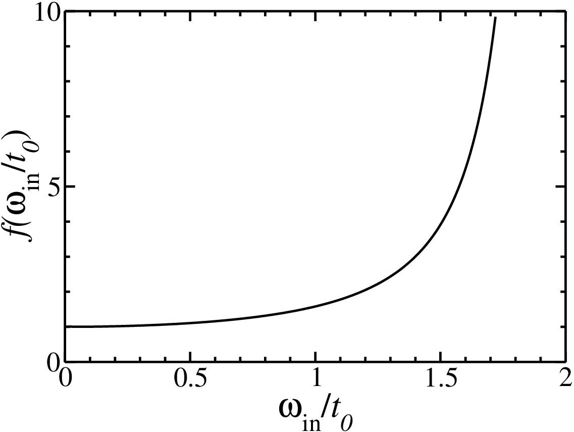
The dimensionless electron-phonon coupling constant is defined as $\lambda_{\Gamma}=(\sqrt{27}/M\omega_{\mathrm{ph}})(t_{0}^{-1}\partial{t}_{0}/\partial{a})^{2}$, which coincides with the definition of Ref. [17] in the tight-binding model. The dimensionless function $f(\omega_{\mathrm{in}}/t_{0})$ is plotted in Fig. 3. In the low-energy limit, $\omega_{\mathrm{in}}\ll{t}_{0}$, its value is $f(0)=1$, as follows from Eq. (3ijla). When the frequency matches the van Hove singularity at the $M$ point of the first Brillouin zone, $\omega_{\mathrm{in}}\approx{2}t_{0}$, the intensity diverges, $f(\omega_{\mathrm{in}}/t_{0})\propto{1}/(\omega_{\mathrm{in}}/t_{0}-2)^{2}$. This divergence is cut off at the scale $|\omega_{\mathrm{in}}-2t_{0}|\sim\max\{\omega_{\mathrm{ph}},\gamma\}$. However, in the absence of a reliable information on electronic relaxation processes in this region of the spectrum, we prefer not to study this issue in detail, leaving the divergence as it is.

First, let us see which electron-hole states contribute the most to the $G$ peak intensity. In principle, for $\omega_{\mathrm{in}}\ll{t}_{0}$ one can imagine three situations. They are illustrated Fig. 4 where the $\pi$ electron dispersion is shown schematically, together with the contributing states. In the situation (a) these are the states whose energies are close to the half of the excitation frequency, the difference $\epsilon_{\mathbf{k}}-\omega_{\mathrm{in}}/2$ being small by some parameter. This was shown to be the case for the $2D$ peak, the second-order overtone of the $D$ peak at 2700 cm^-1, which is fully resonant and $|\epsilon_{\mathbf{k}}-\omega_{\mathrm{in}}/2|\sim\gamma$, where $2\gamma\ll\omega_{\mathrm{in}}$ is the electron inelastic scattering rate [18, 17]. This is also the case for the doubly-resonant $D$ peak at 1350 cm^-1, where $|\epsilon_{\mathbf{k}}-\omega_{\mathrm{in}}/2|\sim\omega_{\mathrm{ph}}\ll\omega_{\mathrm{in}}$ [19, 20]. In the situation (b) the difference $|\epsilon_{\mathbf{k}}-\omega_{\mathrm{in}}/2|\sim\omega_{\mathrm{in}}$ itself, and no small parameter enters. Finally, in the situation (c) the Raman process is contributed by the whole Brillouin zone, $\epsilon_{\mathbf{k}}\sim{t}_{0}$.

A natural guess for the $G$ peak would be the option (a): indeed, there is a contribution from intermediate states that violate energy conservation by the energy $\sim\omega_{\mathrm{ph}}$. However, in Ref. [17] it was found that the main contribution to the integral in Eq. (3h) with only two terms (3ia), (3ib) came from the states $\epsilon_{\mathbf{k}}\sim{t}_{0}$ [option (c)]. In the present work we have seen that this contribution, in fact, is canceled by other terms, missed in Ref. [17], due to the Ward identity. To see that the correct picture for the $G$ peak in fact corresponds to Fig. 4(c), let us consider doped sample, i. e., with the Fermi energy $\epsilon_{F}$ detuned from the Dirac point. Then transitions involving states with $\epsilon_{\mathbf{k}}<|\epsilon_{F}|$ are simply blocked by the Pauli principle, so the lower limit of the integral in Eq. (3ijla) must be set to $|\epsilon_{F}|$. Let us analyze the first term in Eq. (3ijla) (the second term is almost equal to the first, the third one is smaller by a factor $\sim\omega_{\mathrm{ph}}^{2}/\omega_{\mathrm{in}}^{2}$):

The value of the integral is determined entirely by the ratio $|\epsilon_{F}|/\omega_{\mathrm{in}}$, and no other energy scales enter, whether small ($\omega_{\mathrm{ph}}$) or large ($t_{0}$). That is, the value of the integral in Eq. (3ijla) is determined not just by the vicinity of the pole, but by the whole range of energies from $\epsilon_{\mathbf{k}}=0$ to $\epsilon_{\mathbf{k}}\sim\omega_{\mathrm{in}}$. Numerically, when $\epsilon_{F}$ is raised from zero to $\omega_{\mathrm{in}}/4$ (half of the distance to the pole), $|\mathcal{M}^{xxy}|^{2}$ is changed by about 12%.

In other words, the uncertainty in the energy of the electron-hole states, contributing to the process, is of the order of their energy itself ($\sim\omega_{\mathrm{in}}$). By virtue of the energy-time uncertainty principle, the duration of the process (the typical lifetime of the virtual electron-hole pair) is $\sim{1}/\omega_{\mathrm{in}}$. The relevant length scale is thus $v/\omega_{\mathrm{in}}\sim{3}\>\mbox{\AA}$ for $v=10^{8}\>\mbox{cm/s}\approx{7}\>\mbox{eV}\cdot\mbox{\AA}$ and $\omega_{\mathrm{in}}=2\>\mbox{eV}$. The Raman process giving rise to the $G$ peak is thus extremely local in space, involving just a few carbon atoms, as it was noted earlier [21]. Its locality can be also understood from the quasiclassical real-space picture of Raman scattering in graphene [20]. This short length scale should be contrasted to much longer scales responsible for Raman peaks produced according to Fig. 4 (a), for example, the doubly-resonant $D$ peak at 1350 cm^-1 [23, 24, 22, 20].

Another consequence of the cancellation of the contribution from $\epsilon_{\mathbf{k}}\sim{t}_{0}$ is the frequency dependence of $I_{G}$. The standard textbook dependence $I\propto\omega^{4}$ (for simplicity we assume $\omega_{\mathrm{in}}\approx\omega_{\mathrm{out}}$) is obtained for systems whose excited states have energies much higher than $\omega_{\mathrm{in}}$ [25]. The $\omega^{4}$ dependence, suggested in Ref. [17], was essentially of the same origin: it was assumed that the main contribution to the process came from states in the bulk of the Brillouin zone, and thus with high energies. As we have seen, this conclusion is wrong, and the relevant states have energies $\epsilon_{\mathbf{k}}\sim\omega_{\mathrm{in}}$. This remains true even at low frequencies, as the electronic spectrum in graphene has no (or almost no) gap. As a result, at low frequencies the dependence is $\propto\omega_{\mathrm{in}}^{2}$, as seen from Eq. (3ijlm). Nevertheless, a recent measurement of Raman peak intensities performed on graphite nanocrystallites gives a $\omega_{\mathrm{in}}^{4}$ dependence [15, 26]. For comparison, we plot $I_{G}$ from Eq. (3ijlm) together with two curves $\propto\omega_{\mathrm{in}}^{4}$ with two different coefficients in Fig. 5.

Let us compare $I_{G}$ to the intensities of other peaks which have been calculated theoretically and measured experimentally. The $D$ peak at 1350 cm^-1 is due to emission of the scalar $A_{1}$ phonons with wave vectors near the $K$ point. Due to momentum conservation, the $D$ peak is activated by defects or edges. For a defect-free graphene flake of the size $L_{a}$ its intensity is given by [20]

Here $\omega_{D}\approx{0}.17\>\mbox{eV}$ and $\lambda_{K}$ are the frequency and the dimensionless electron-phonon coupling constant for the corresponding phonons, $v\approx{7}\>\mbox{eV}\cdot\mbox{\AA}$ is the electron velocity (the slope of the Dirac cones), $2\gamma$ is the electron inelastic scattering rate, $L_{x}L_{y}$ is the area of the excitation laser spot, and $C$ is a numerical coefficient which depends on the shape of the flake and the character of the edges. We take $\lambda_{\Gamma}=0.03$, as obtained from the doping dependence of the $G$ peak frequency [6, 7], and $\lambda_{K}/\lambda_{\Gamma}=3$ as extracted from the ratio of intensities of the intensities of the $2D$ peak at $2700\>\mbox{cm}^{-1}$ and the $2D^{\prime}$ peak at $3250\>\mbox{cm}^{-1}$ [17]. Let us assume the inelastic scattering rate to be dominated by electron-phonon scattering (which is a lower bound), then it can be estimated as $\gamma=(\lambda_{\Gamma}+\lambda_{K})\omega_{\mathrm{in}}/8$ [18]. For a small flake, Eq. (3ijlm) should be weighted by the ratio of the area of the flake to the excitation spot area. If we take an ideal hexagonal flake with armchair edges (which definitely represents an upper bound for $I_{D}$), then its area is $L_{a}^{2}\sqrt{27}/8$ and $C=4$. For a round flake of the diameter $L_{a}$ with atomically rough edges the area is $\pi{L}_{a}^{2}/4$ and $C=\pi^{2}/18$, i. e., $I_{D}$ is about 10 times smaller than for the ideal flake. Taking $\omega_{\mathrm{in}}=2\>\mbox{eV}$ and using the low-frequency limit of Eq. (3ijlm), $f(\omega_{\mathrm{in}}/t_{0})=1$, we obtain $I_{D}/I_{G}\approx(300-3000\>\mbox{nm})/L_{a}$. The experimentally found intensity is $I_{D}/I_{G}=(560\>\mbox{nm}\cdot\mbox{eV}^{4})/(L_{a}\omega_{\mathrm{in}}^{4})$ [15, 26], which at $\omega_{\mathrm{in}}=2\>\mbox{eV}$ gives an almost 10 times smaller value than the calculated one for a flake with rough edges.

We can also consider $2D$ peak at $2700\>\mbox{cm}^{-1}$, whose intensity was calculated to be [18, 17]

For the same values as above we obtain $I_{2D}/I_{G}\approx{150}$. The experimental value for graphene samples on a substrate is typically $I_{2D}/I_{G}\approx{5}$ [5, 12]. For suspended samples the ratio can be $I_{2D}/I_{G}\approx{9}$ [27] and even $I_{2D}/I_{G}\approx{17}$ [28]. Still, the experimental ratio is about 10 times smaller than the calculated one.

Thus, the theory overestimates both $I_{2D}/I_{G}$ and $I_{D}/I_{G}$ by about an order of magnitude. It seems more reasonable to assume that Eq. (3ijlm) for $I_{G}$ should be blamed for this discrepancy, rather than expressions for $I_{D}$ and $I_{2D}$. Indeed, as discussed above, $I_{D}$ and $I_{2D}$ are determined by just a few material parameters (electron-phonon coupling constants, electronic velocity, etc.) which have been calculated by different methods and measured in many independent experiments. Moreover, corrections to Eq. (3ijlp) due to the trigonal warping and electron-hole asymmetry have been estimated in Ref. [17] and turned out to be small. At the same time, the parameters determining $I_{G}$ (electronic trigonal warping, electron-phonon coupling anisotropy) are not really known, the validity of the tight-binding model at sufficiently high energies is questionable, and even the calculated frequency dependence of $I_{G}$ does not seem to agree with the experiment.

Still, what is the main source of such a strong discrepancy? Is it possible that $\omega_{\mathrm{in}}=2\>\mbox{eV}$ is already sufficiently close to the singularity at $\omega_{\mathrm{in}}=2t_{0}$, so that the dependence of $I_{G}$ on $\omega_{\mathrm{in}}$ is noticeably steeper than $\omega^{2}$, and the value of $I_{G}$ is higher than that predicted by the low-frequency asymptotics? On the one hand, the nearest-neighbor tight-binding model with $t_{0}\approx{3}\>\mbox{eV}$ seems to describe the band structure reasonably well in the energy range of interest, as is seen from its comparison with the results obtained by angle-resolved photoemission spectroscopy [29]. Then the energy of electron-hole separation at the $M$ point is $2t_{0}\approx{6}\>\mbox{eV}$ and $\omega_{\mathrm{in}}/t_{0}=0.6$ is quite close to the low-energy limit, as seen from Fig. 3. On the other hand, a recent ab initio calculation of the band structure of graphite gives the electron-hole separation at the $M$ point about 4 eV [30]. Also, the anisotropy of the electron-phonon coupling may be stronger than that obtained from the nearest-neighbor tight-binding model [31]. In addition, the spectrum of electron-hole excitations can be modified by excitonic effects: the Coulomb attraction between the electron and the hole lowers the energy of the excitation with respect to its non-interacting value, so that the singularity in $I_{D}$ should be at a lower frequency. The author is aware of only one study of excitonic effects in the optical response of monolayer graphene; within the Dirac model it was shown that excitonic effects result in a weak feature at the border of the electron-hole continuum [32]. Their importance for optical excitation of electrons near the $M$ point of the first Brillouin zone remains to be studied. Also, a direct measurement of the energy corresponding to the singularity by an excitation in the ultraviolet frequency range would shed light on this issue.

We have calculated the frequency-integrated intensity of the Raman $G$ peak in monolayer graphene using the nearest-neighbor tight-binding model for electrons. The resulting intensity is determined by the trigonal warping of the electronic bands and the anisotropy of the electron-phonon coupling, and is proportional to the second power of the excitation frequency. Comparison to the intensities of other peaks, which have been measured experimentally and calculated theoretically, suggests that the present calculation underestimates $I_{G}$ by about an order of magnitude.

References

- [1] Mandelshtam L I and Landsberg G S 1928 Z. Phys. 50 169; Raman C V and Krishnan K S 1928 Nature 121 501
- [2] Reich S and Thomsen C 2004 Phil. Trans. R. Soc. Lond. A 362 2271
- [3] Dresselhaus M S, Dresselhaus G, Saito R and Jorio A 2005 Phys. Rep. 409 47
- [4] Novoselov K S, Geim A K, Morozov S V, Jiang D, Zhang Y, Dubonos S V, Grigorieva I V and Firsov A A 2004 Science 306 666
- [5] Ferrari A C, Meyer J C, Scardaci V, Casiraghi C, Lazzeri M, Mauri F, Piscanec S, Jiang D, Novoselov K S, Roth S and Geim A K 2006 Phys. Rev. Lett.97 187401
- [6] Yan J, Zhang Y, Kim P and Pinczuk A 2007 Phys. Rev. Lett.98 166802
- [7] Pisana S, Lazzeri M, Casiraghi C, Novoselov K S, Geim A K, Ferrari A C and Mauri F 2007 Nature Mat. 6 198
- [8] Das A, Pisana S, Chakraborty B, Piscanec S, Saha S K, Waghmare U V, Novoselov K S, Krishnamurhthy H R, Geim A K, Ferrari A C and Sood A K, 2008 Nature Nanotechnology 3 210
- [9] Das A, Chakraborty B, Piscanec S, Pisana S, Sood A K and Ferrari A C 2009 Phys. Rev.B 79 155417
- [10] Mohiuddin T M G, Lombardo A, Nair R R, Bonetti A, Savini G, Jalil R, Bonini N, Basko D M, Galiotis C, Marzari N, Novoselov K S, Geim A K and Ferrari A C 2009 Phys. Rev.B 79 205433
- [11] Huang M, Yan H, Chen C, Song D, Heinz T F and Hone J 2009 Proc. Natl. Acad. Sci. USA 106 7304
- [12] Ni Z H, Yu T, Lu Y H, Wang Y Y, Feng Y P and Shen Z X 2008 ACS Nano 2 2301
- [13] Elias D C, Nair R R, Mohiuddin T M G, Morozov S V, Blake P, Halsall M P, Ferrari A C, Boukhvalov D W, Katsnelson M I, Geim A K and Novoselov K S, 2009 Science 323 610
- [14] Ryu S, Han M Y, Maultzsch J, Heinz T F, Kim P, Steigerwald M L and Brus L E, 2008 Nano Lett. 8 4597
- [15] Cançado L G, Takai K, Enoki T, Endo M, Kim Y A, Mizusaki H, Jorio A, Coelho L N, Magalhães-Paniago R and Pimenta M A 2006 Appl. Phys. Lett. 88 163106
- [16] Tuinstra F and Koenig J L 1970 J. Chem. Phys. 53 1126
- [17] Basko D M 2008 Phys. Rev. B 78 125418
- [18] Basko D M 2007 Phys. Rev. B 76 081405(R); 2009 Phys. Rev. B 79 209903(E)
- [19] Thomsen C and Reich S 2000 Phys. Rev. Lett. 85 5214
- [20] Basko D M 2009 Phys Rev. B 79 205428
- [21] Ferrari A C and Robertson J 2000 Phys. Rev. B 61 14095
- [22] Casiraghi C, Hartschuh A, Qian H, Piscanec S, Georgi C, Novoselov K S, Basko D M and Ferrari A C 2009 Nano Lett. 9 1433
- [23] Cançado L G, Beams R and Novotny L 2008 arXiv:0802.3709
- [24] Gupta A K, Russin T J, Gutièrrez H R and Eklund P C 2009 ACS Nano 3 45
- [25] Long D A 1977 Raman Spectroscopy (McGraw-Hill)
- [26] Cançado L G, Jorio A and Pimenta M A 2007 Phys. Rev. B 76 064304
- [27] Ni Z H, Yu T, Luo Z Q, Wang Y Y, Liu L, Wong C P, Miao J, Huang W and Shen Z X 2009 ACS Nano 3 569
- [28] Berciaud S, Ryu S, Brus L E and Heinz T F 2009 Nano Lett. 9 346
- [29] Bostwick A, Ohta T, McChesney J L, Seyller T, Horn K and Rotenberg E 2007 Solid State Commun. 143 63
- [30] Grüneis A, Attaccalite C, Wirtz L, Shiozawa H, Saito R, Pichler T and Rubio A 2008 Phys. Rev. B 78 205425
- [31] Park C-H, Giustino F, McChesney J L, Bostwick A, Ohta T, Rotenberg E, Cohen M L and Louie S G 2008 Phys. Rev. B 77 113410
- [32] Gangadharaiah S, Farid A M and Mishchenko E G 2008 Phys. Rev. Lett. 100 166802