跳到论文正文
W Papers独立论文阅读器 arXiv:0910.0473 论文正文 计算阅读时间 · 0%
引用这篇论文根据当前论文元数据生成,正式投稿前建议核对。


License: arXiv.org perpetual non-exclusive license
arXiv:0910.0473v1 [hep-ph] 02 Oct 2009

Two-loop soft anomalous dimensions with massive and massless quarks

Nikolaos Kidonakis Affiliation: Kennesaw State University, Kennesaw, GA 30144, USA
Abstract

I present results for two-loop soft anomalous dimensions, which are derived from dimensionally regularized diagrams with eikonal quark lines and control soft-gluon emission in hard-scattering processes. Detailed results for the UV poles of the eikonal integrals are shown for massive quarks, and the massless limit is also taken. The construction of soft anomalous dimensions at two-loops allows soft-gluon resummations at NNLL accuracy.

I Introduction

Soft-gluon resummation formalisms for top quark production and other hard scattering cross sections beyond leading logarithms are formulated in terms of exponentials of soft anomalous dimensions that control noncollinear soft-gluon emission (see e.g. [1]). The calculations of these anomalous dimensions [2, 3] are performed using the eikonal approximation, which is valid for descibing the emission of soft gluons from partons in the hard scattering. The approximation leads to a simplified form of the Feynman rules by removing the Dirac matrices from the calculation. When the gluon momentum, kk, goes to zero, the Feynman rule for the quark-gluon vertex reduces to gs​TFc​vμ/v⋅kg_{s}T_{F}^{c}v^{\mu}/v\cdot k with vv a dimensionless velocity vector.

Here we calculate diagrams and derive the soft anomalous dimension for top quark pair production via e+​e−→t​t¯e^{+}e^{-}\rightarrow t{\bar{t}} through two loops [3]. We also discuss the massless limit and extensions to other processes.

Writing the soft anomalous dimension ΓS\Gamma_{S} as a series in αs\alpha_{s}

ΓS=αsπ​ΓS(1)+(αsπ)2​ΓS(2)+⋯\Gamma_{S}=\frac{\alpha_{s}}{\pi}\Gamma_{S}^{(1)}+\left(\frac{\alpha_{s}}{\pi}\right)^{2}\Gamma_{S}^{(2)}+\cdots (1)

we calculate the one- and two-loop expressions for ΓS\Gamma_{S}. We use the Feynman gauge and we employ dimensional regularization with n=4−ϵn=4-\epsilon dimensions. The soft anomalous dimension can be determined from the coefficients of the ultraviolet (UV) poles of the eikonal diagrams.

We do not include the color factors in the individual diagrams below, but take them into account when assembling all the pieces together in the last section. The Appendix lists some of the integrals calculated for the evaluation of the diagrams.

II One-loop diagrams
Refer to caption
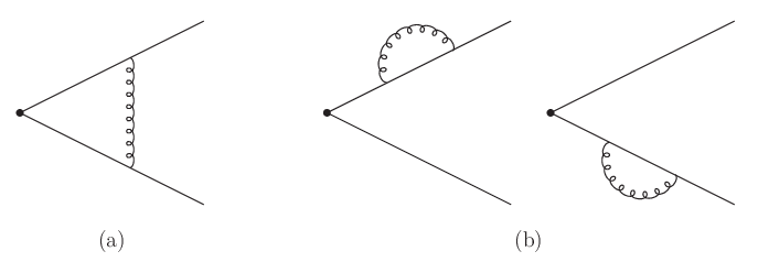
Figure 1: One-loop diagrams with heavy-quark eikonal lines.

In this section we calculate the one-loop diagrams in Fig. 1. We define β=1−4​m2/s\beta=\sqrt{1-4m^{2}/s} with mm the heavy quark mass and ss the squared c.m. energy. We label the two heavy quark lines by ii and jj. Using the relation v=p​2/sv=p\,{\sqrt{2/s}}, with pp the momentum, we have vi2=vj2=(1−β2)/2v_{i}^{2}=v_{j}^{2}=(1-\beta^{2})/2 and vi⋅vj=(1+β2)/2v_{i}\cdot v_{j}=(1+\beta^{2})/2.

We begin with the integral I1​aI_{1a} for the diagram in Fig. 1(a) given by

I1​a=gs2​∫dn​k(2​π)n​(−i)​gμ​νk2​viμvi⋅k​(−vjν)(−vj⋅k).I_{1a}=g_{s}^{2}\int\frac{d^{n}k}{(2\pi)^{n}}\frac{(-i)g_{\mu\nu}}{k^{2}}\frac{v_{i}^{\mu}}{v_{i}\cdot k}\,\frac{(-v_{j}^{\nu})}{(-v_{j}\cdot k)}\,. (2)

Using Feynman parameterization and after several manipulations and separation of UV and infrared (IR) singularities, we find through Eq. (Appendix) the UV poles

I1​a=αsπ​(1+β2)2​β​1ϵ​ln⁡(1−β1+β).I_{1a}=\frac{\alpha_{s}}{\pi}\frac{(1+\beta^{2})}{2\,\beta}\frac{1}{\epsilon}\ln\left(\frac{1-\beta}{1+\beta}\right)\,. (3)

Next we calculate the one-loop self-energy diagrams in Fig. 1(b) given by

I1​b=gs2​∫dn​k(2​π)n​(−i)​gμ​νk2​viμvi⋅(k′−k)​viνvi⋅k′.I_{1b}=g_{s}^{2}\int\frac{d^{n}k}{(2\pi)^{n}}\frac{(-i)g_{\mu\nu}}{k^{2}}\frac{v_{i}^{\mu}}{v_{i}\cdot(k^{\prime}-k)}\,\frac{v_{i}^{\nu}}{v_{i}\cdot k^{\prime}}\,. (4)

Here we have introduced the regulator k′k^{\prime}, i.e. the external quark momentum is pi+k′p_{i}+k^{\prime}, so as to use the eikonal rules. We then expand the above expression around vi⋅k′=0v_{i}\cdot k^{\prime}=0 at constant ϵ\epsilon. The expansion gives an irrelevant 1/vi⋅k′1/v_{i}\cdot k^{\prime} term, a constant term, and linear and higher-order terms in vi⋅k′v_{i}\cdot k^{\prime} which vanish when setting k′=0k^{\prime}=0. The remaining term is then

I1​b=i​gs2​vi2(2​π)n​∫dn​kk2​(vi⋅k)2.I_{1b}=\frac{i\,g_{s}^{2}\,v_{i}^{2}}{(2\pi)^{n}}\int\frac{d^{n}k}{k^{2}\,(v_{i}\cdot k)^{2}}\,. (5)

We isolate the UV poles and using Eq. (70) we find

I1​b=αsπ​1ϵ.I_{1b}=\frac{\alpha_{s}}{\pi}\frac{1}{\epsilon}\,. (6)

The one-loop soft anomalous dimension is then read off the coefficient of the UV poles of the one-loop diagrams through

CF​[I1​a+I1​b]=−αsπ​ΓS(1)ϵC_{F}[I_{1a}+I_{1b}]=-\frac{\alpha_{s}}{\pi}\frac{\Gamma_{S}^{(1)}}{\epsilon} (7)

which gives

ΓS(1)=CF​[−(1+β2)2​β​ln⁡(1−β1+β)−1]\Gamma_{S}^{(1)}=C_{F}\left[-\frac{(1+\beta^{2})}{2\,\beta}\ln\left(\frac{1-\beta}{1+\beta}\right)-1\right] (8)

with CF=(Nc2−1)/(2​Nc)C_{F}=(N_{c}^{2}-1)/(2N_{c}) the color factor.

When expressed in terms of the cusp angle γ=cosh−1⁡(vi⋅vj/vi2​vj2)=ln⁡[(1+β)/(1−β)]\gamma=\cosh^{-1}\left(v_{i}\cdot v_{j}/\sqrt{v_{i}^{2}v_{j}^{2}}\right)=\ln[(1+\beta)/(1-\beta)] this becomes ΓS(1)=CF​(γ​coth⁡γ−1)\Gamma_{S}^{(1)}=C_{F}(\gamma\coth\gamma-1) and is also known as a cusp anomalous dimension [4, 5].

III Two-loop vertex diagrams

Refer to caption
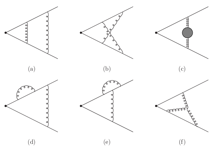
Figure 2: Two-loop vertex diagrams with heavy-quark eikonal lines.

The two-loop diagrams can be separated into two groups, shown in Fig. 2 and 3. The calculations are challenging due to the presence of a heavy quark mass and they involve multiple complicated integrals and delicate separations of infrared and ultraviolet poles, which by construction of the soft function are opposites of each other [2]. The analytical structure of the results involves logarithms and polylogarithms.

In this section we calculate the two-loop vertex diagrams of Fig. 2. We also have to include the one-loop counterterms to these diagrams. We will denote by I2′I^{\prime}_{2} the diagrams in Fig. 2 and by I2c.t.I^{c.t.}_{2} their counterterms. The total contribution will then be I2=I2′+I2c.t.I_{2}=I^{\prime}_{2}+I^{c.t.}_{2}.

We find it convenient to define

Mβ\displaystyle M_{\beta} =\displaystyle= (4​ln⁡2+ln⁡π−γE−i​π)​ln⁡(1−β1+β)\displaystyle\left(4\ln 2+\ln\pi-\gamma_{E}-i\pi\right)\ln\left(\frac{1-\beta}{1+\beta}\right) (9)
+12​ln2⁡(1+β)−12​ln2⁡(1−β)\displaystyle{}+\frac{1}{2}\ln^{2}(1+\beta)-\frac{1}{2}\ln^{2}(1-\beta)
−Li2​(1+β2)+Li2​(1−β2).\displaystyle{}-{\rm Li}_{2}\left(\frac{1+\beta}{2}\right)+{\rm Li}_{2}\left(\frac{1-\beta}{2}\right)\,.

III.1 I2​aI_{2a} and I2​bI_{2b}

In this section we calculate the integrals I2​aI_{2a} and I2​bI_{2b} for the two-loop diagrams in Figs. 2(a) and 2(b). Note that there is no counterterm for diagram 2(b), so I2​b=I2​b′I_{2b}=I^{\prime}_{2b}.

Diagram 2(b) is given by

I2​b=gs4​∫dn​k1(2​π)n​dn​k2(2​π)n​(−i)​gμ​νk12​(−i)​gρ​σk22\displaystyle\hskip-34.1433ptI_{2b}=g_{s}^{4}\int\frac{d^{n}k_{1}}{(2\pi)^{n}}\frac{d^{n}k_{2}}{(2\pi)^{n}}\frac{(-i)g_{\mu\nu}}{k_{1}^{2}}\frac{(-i)g_{\rho\sigma}}{k_{2}^{2}}
×viμvi⋅k1​viρvi⋅(k1+k2)​(−vjν)−vj⋅(k1+k2)​(−vjσ)−vj⋅k2.\displaystyle\hskip-25.60747pt\times\frac{v_{i}^{\mu}}{v_{i}\cdot k_{1}}\frac{v_{i}^{\rho}}{v_{i}\cdot(k_{1}+k_{2})}\frac{(-v_{j}^{\nu})}{-v_{j}\cdot(k_{1}+k_{2})}\frac{(-v_{j}^{\sigma})}{-v_{j}\cdot k_{2}}. (10)

Now, we begin with the k2k_{2} integral and use Feynman parameterization. Performing first the k2k_{2} integration and then an integration over one of the parameters, we have

I2​b=−i​αs2π2​ 2−4+ϵ​π−2+3​ϵ2​Γ​(1−ϵ2)​Γ​(1+ϵ)\displaystyle\hskip-8.53581ptI_{2b}=-i\frac{\alpha_{s}^{2}}{\pi^{2}}\,2^{-4+\epsilon}\,\pi^{-2+3\frac{\epsilon}{2}}\,\Gamma\left(1-\frac{\epsilon}{2}\right)\,\Gamma(1+\epsilon)
×(1+β2)2​∫01d​z​∫01d​y​(1−y)−ϵ\displaystyle\times(1+\beta^{2})^{2}\int_{0}^{1}dz\int_{0}^{1}dy\,(1-y)^{-\epsilon}
×[2​β2​(1−y)2​z2−2​β2​(1−y)​z−(1−β2)2]−1+ϵ2\displaystyle\times\left[2\beta^{2}(1-y)^{2}z^{2}-2\beta^{2}(1-y)z-\frac{(1-\beta^{2})}{2}\right]^{-1+\frac{\epsilon}{2}}
×∫dn​k1k12​vi⋅k1​[((vi−vj)​z+vj)⋅k1]1+ϵ.\displaystyle\times\int\frac{d^{n}k_{1}}{k_{1}^{2}\,v_{i}\cdot k_{1}\,\left[\left((v_{i}-v_{j})z+v_{j}\right)\cdot k_{1}\right]^{1+\epsilon}}\,. (11)

Next we proceed with the k1k_{1} integral

∫dn​k1k12​vi⋅k1​[((vi−vj)​z+vj)⋅k1]1+ϵ=−i​(−1)−3​ϵ2\displaystyle\hskip-14.22636pt\int\frac{d^{n}k_{1}}{k_{1}^{2}\,v_{i}\cdot k_{1}\,\left[\left((v_{i}-v_{j})z+v_{j}\right)\cdot k_{1}\right]^{1+\epsilon}}=-i(-1)^{-3\frac{\epsilon}{2}}
×22+3​ϵ​π2−ϵ2​Γ⁡(1+3​ϵ2)Γ⁡(1+ϵ)​∫01d​x1​x1−1+2​ϵ​(1−x1)−1−2​ϵ\displaystyle\hskip-8.53581pt\times 2^{2+3\epsilon}\pi^{2-\frac{\epsilon}{2}}\frac{\Gamma\left(1+\frac{3\epsilon}{2}\right)}{\Gamma(1+\epsilon)}\int_{0}^{1}dx_{1}x_{1}^{-1+2\epsilon}(1-x_{1})^{-1-2\epsilon}
×∫01dx2(1−x2)ϵ{[x2vi\displaystyle\hskip-8.53581pt\times\int_{0}^{1}dx_{2}(1-x_{2})^{\epsilon}\left\{\left[x_{2}v_{i}\right.\right.
+(1−x2)((vi−vj)z+vj)]2}−1−3​ϵ2.\displaystyle\hskip 28.45274pt\left.\left.+(1-x_{2})\left((v_{i}-v_{j})z+v_{j}\right)\right]^{2}\right\}^{-1-3\frac{\epsilon}{2}}. (12)

The integral over x1x_{1} contains both UV and IR singularities. We isolate the UV singularities via

∫01d​x1​x1−1+2​ϵ​(1−x)−1−2​ϵ=∫01d​x1​x1−1+2​ϵ\displaystyle\hskip-31.29802pt\int_{0}^{1}dx_{1}\,x_{1}^{-1+2\epsilon}(1-x)^{-1-2\epsilon}=\int_{0}^{1}dx_{1}\,x_{1}^{-1+2\epsilon}
+∫01dx1x1−1+2​ϵ[(1−x)−1−2​ϵ−1]=12​ϵ+IR.\displaystyle\hskip-28.45274pt{}+\int_{0}^{1}dx_{1}\,x_{1}^{-1+2\epsilon}\left[(1-x)^{-1-2\epsilon}-1\right]=\frac{1}{2\epsilon}+{\rm IR}. (13)

We set ϵ=0\epsilon=0 in the integral over x2x_{2} since it is UV finite. We thus find the UV poles of the k1k_{1} integral

∫dn​k1k12​vi⋅k1​[((vi−vj)​z+vj)⋅k1]1+ϵ=−i​ 2​π2​1ϵ\displaystyle\hskip-28.45274pt\int\frac{d^{n}k_{1}}{k_{1}^{2}\,v_{i}\cdot k_{1}\,\left[\left((v_{i}-v_{j})z+v_{j}\right)\cdot k_{1}\right]^{1+\epsilon}}=-i\,2\pi^{2}\frac{1}{\epsilon}
×1β⁡(1−z)​[tanh−1⁡(β⁡(1−2​z))−tanh−1⁡(−β)].\displaystyle\hskip-22.76219pt\times\frac{1}{\beta(1-z)}\left[\tanh^{-1}(\beta(1-2z))-\tanh^{-1}(-\beta)\right]\,. (14)

Using this result in the expression for I2​bI_{2b}, Eq. (11), and performing the yy and zz integrals, we find

I2​b=αs2π2(1+β2)28​β21ϵ{−13ln3(1−β1+β)\displaystyle\hskip-17.07164ptI_{2b}=\frac{\alpha_{s}^{2}}{\pi^{2}}\frac{(1+\beta^{2})^{2}}{8\,\beta^{2}}\frac{1}{\epsilon}\left\{-\frac{1}{3}\ln^{3}\left(\frac{1-\beta}{1+\beta}\right)\right.
−ln⁡(1−β1+β)​[Li2​((1−β)2(1+β)2)+ζ2]\displaystyle\hskip 42.67912pt{}-\ln\left(\frac{1-\beta}{1+\beta}\right)\left[{\rm Li}_{2}\left(\frac{(1-\beta)^{2}}{(1+\beta)^{2}}\right)+\zeta_{2}\right]
+Li3((1−β)2(1+β)2)−ζ3}.\displaystyle\hskip 42.67912pt\left.{}+{\rm Li}_{3}\left(\frac{(1-\beta)^{2}}{(1+\beta)^{2}}\right)-\zeta_{3}\right\}. (15)

Diagrams 2(a) and 2(b) are related through the equation I2​a′+I2​b=12​I1​a2I^{\prime}_{2a}+I_{2b}=\frac{1}{2}I_{1a}^{2} (where we need to keep UV poles and constant terms in I1​aI_{1a}) from which we can calculate I2​a′I^{\prime}_{2a}. The one-loop counterterm to I2​aI_{2a} is

I2​ac.t.=αs2π2(1+β2)28​β2{−2ϵ2ln2(1−β1+β)\displaystyle\hskip-42.67912ptI_{2a}^{c.t.}=\frac{\alpha_{s}^{2}}{\pi^{2}}\frac{(1+\beta^{2})^{2}}{8\,\beta^{2}}\left\{-\frac{2}{\epsilon^{2}}\ln^{2}\left(\frac{1-\beta}{1+\beta}\right)\right.
−1ϵ​M​(β)​ln⁡(1−β1+β).\displaystyle\hskip 56.9055pt-\frac{1}{\epsilon}M(\beta)\ln\left(\frac{1-\beta}{1+\beta}\right)\,. (16)

Then we find the simple relation

I2​a+I2​b=αs2π2​(1+β2)28​β2​(−1)ϵ2​ln2⁡(1−β1+β).I_{2a}+I_{2b}=\frac{\alpha_{s}^{2}}{\pi^{2}}\frac{(1+\beta^{2})^{2}}{8\,\beta^{2}}\frac{(-1)}{\epsilon^{2}}\ln^{2}\left(\frac{1-\beta}{1+\beta}\right)\,. (17)

III.2 I2​cI_{2c}

In this section we calculate the integrals for the three diagrams represented by Fig. 2(c). The blob represents a quark, gluon, or ghost loop. Note that an additional diagram with a four-gluon vertex vanishes.

The quark-loop diagram is given by

I2​c​q′=(−1)​nf​gs4​∫dn​k(2​π)n​dn​l(2​π)n​viμvi⋅k​(−vjρ)(−vj⋅k)\displaystyle\hskip-28.45274ptI^{\prime}_{2cq}=(-1)n_{f}g_{s}^{4}\int\frac{d^{n}k}{(2\pi)^{n}}\frac{d^{n}l}{(2\pi)^{n}}\frac{v_{i}^{\mu}}{v_{i}\cdot k}\frac{(-v_{j}^{\rho})}{(-v_{j}\cdot k)}
×(−i)​gμ​νk2​(−i)​gρ​σk2​Tr​[−i​γν​il/l2​(−i)​γσ​i​(l/−k/)(l−k)2].\displaystyle\hskip-22.76219pt\times\frac{(-i)g_{\mu\nu}}{k^{2}}\frac{(-i)g_{\rho\sigma}}{k^{2}}{\rm Tr}\left[-i\gamma^{\nu}\frac{il\!\!/}{l^{2}}(-i)\gamma^{\sigma}i\frac{(l\!\!/-k\!\!/)}{(l-k)^{2}}\right]. (18)

After several steps, and using Eq. (71), the final result for the UV poles of I2​c​q′I^{\prime}_{2cq} is

I2​c​q′=αs2π2nf(1+β2)6​β{−1ϵ2ln(1−β1+β)\displaystyle\hskip-34.1433ptI^{\prime}_{2cq}=\frac{\alpha_{s}^{2}}{\pi^{2}}n_{f}\frac{(1+\beta^{2})}{6\,\beta}\left\{-\frac{1}{\epsilon^{2}}\ln\left(\frac{1-\beta}{1+\beta}\right)\right.
−1ϵ[56ln(1−β1+β)+Mβ]}\displaystyle\hskip 48.36967pt\left.{}-\frac{1}{\epsilon}\left[\frac{5}{6}\ln\left(\frac{1-\beta}{1+\beta}\right)+M_{\beta}\right]\right\} (19)

with nfn_{f} the number of light quark flavors. The one-loop counterterm is

I2​c​qc.t.=αs2π2​nf​(1+β2)6​β​{2ϵ2​ln⁡(1−β1+β)+1ϵ​Mβ}.I_{2cq}^{c.t.}=\frac{\alpha_{s}^{2}}{\pi^{2}}n_{f}\frac{(1+\beta^{2})}{6\,\beta}\left\{\frac{2}{\epsilon^{2}}\ln\left(\frac{1-\beta}{1+\beta}\right)+\frac{1}{\epsilon}M_{\beta}\right\}\,. (20)

Then the sum I2​c​q=I2​c​q′+I2​c​qc.t.I_{2cq}=I^{\prime}_{2cq}+I_{2cq}^{c.t.} gives

I2​c​q=αs2π2​nf​(1+β2)6​β​[1ϵ2−56​ϵ]​ln⁡(1−β1+β).I_{2cq}=\frac{\alpha_{s}^{2}}{\pi^{2}}n_{f}\frac{(1+\beta^{2})}{6\,\beta}\left[\frac{1}{\epsilon^{2}}-\frac{5}{6\,\epsilon}\right]\ln\left(\frac{1-\beta}{1+\beta}\right). (21)

Next we calculate the integral for the gluon-loop diagram given by

I2​c​g​l′=12​gs4​∫dn​k(2​π)n​dn​l(2​π)n​viμvi⋅k​(−vjν)(−vj⋅k)\displaystyle\hskip-11.38109ptI^{\prime}_{2cgl}=\frac{1}{2}g_{s}^{4}\int\frac{d^{n}k}{(2\pi)^{n}}\frac{d^{n}l}{(2\pi)^{n}}\frac{v_{i}^{\mu}}{v_{i}\cdot k}\frac{(-v_{j}^{\nu})}{(-v_{j}\cdot k)}
×(−i)​gμ​μ′k2​(−i)​gρ​ρ′l2​(−i)​gσ​σ′(k−l)2​(−i)​gν​ν′k2\displaystyle\times\frac{(-i)g_{\mu\mu^{\prime}}}{k^{2}}\frac{(-i)g_{\rho\rho^{\prime}}}{l^{2}}\frac{(-i)g_{\sigma\sigma^{\prime}}}{(k-l)^{2}}\frac{(-i)g_{\nu\nu^{\prime}}}{k^{2}}
×[gμ′​ρ​(k+l)σ+gρ​σ​(k−2​l)μ′+gσ​μ′​(−2​k+l)ρ]\displaystyle\times\left[g^{\mu^{\prime}\rho}(k+l)^{\sigma}+g^{\rho\sigma}(k-2l)^{\mu^{\prime}}+g^{\sigma\mu^{\prime}}(-2k+l)^{\rho}\right]
×[gρ′​ν′(l+k)σ′+gν′​σ′(−2k+l)ρ′\displaystyle\times\left[g^{\rho^{\prime}\nu^{\prime}}(l+k)^{\sigma^{\prime}}+g^{\nu^{\prime}\sigma^{\prime}}(-2k+l)^{\rho^{\prime}}\right.
+gσ′​ρ′(k−2l)ν′].\displaystyle\hskip 85.35826pt\left.{}+g^{\sigma^{\prime}\rho^{\prime}}(k-2l)^{\nu^{\prime}}\right]. (22)

Using Eq. (71) we find for the UV poles of I2​c​g​l′I^{\prime}_{2cgl},

I2​c​g​l′=αs2π21996(1+β2)β{−1ϵ2ln(1−β1+β)\displaystyle\hskip-34.1433ptI^{\prime}_{2cgl}=\frac{\alpha_{s}^{2}}{\pi^{2}}\frac{19}{96}\frac{(1+\beta^{2})}{\beta}\left\{-\frac{1}{\epsilon^{2}}\ln\left(\frac{1-\beta}{1+\beta}\right)\right.
−1ϵ[5857ln(1−β1+β)+Mβ]}.\displaystyle\hskip 42.67912pt\left.-\frac{1}{\epsilon}\left[\frac{58}{57}\ln\left(\frac{1-\beta}{1+\beta}\right)+M_{\beta}\right]\right\}. (23)

The one-loop counterterm is

I2​c​g​lc.t.=αs2π2​1996​(1+β2)β​{2ϵ2​ln⁡(1−β1+β)+1ϵ​Mβ}.I_{2cgl}^{c.t.}=\frac{\alpha_{s}^{2}}{\pi^{2}}\frac{19}{96}\frac{(1+\beta^{2})}{\beta}\left\{\frac{2}{\epsilon^{2}}\ln\left(\frac{1-\beta}{1+\beta}\right)+\frac{1}{\epsilon}M_{\beta}\right\}. (24)

Then

I2​c​g​l=αs2π2​1996​(1+β2)β​{1ϵ2−5857​ϵ}​ln⁡(1−β1+β).I_{2cgl}=\frac{\alpha_{s}^{2}}{\pi^{2}}\frac{19}{96}\frac{(1+\beta^{2})}{\beta}\left\{\frac{1}{\epsilon^{2}}-\frac{58}{57\,\epsilon}\right\}\ln\left(\frac{1-\beta}{1+\beta}\right). (25)

Last we calculate the integral for the ghost-loop diagram given by

I2​c​g​h′=(−1)​gs4​∫dn​k(2​π)n​dn​l(2​π)n​viμvi⋅k​(−vjρ)(−vj⋅k)\displaystyle\hskip-28.45274ptI^{\prime}_{2cgh}=(-1)g_{s}^{4}\int\frac{d^{n}k}{(2\pi)^{n}}\frac{d^{n}l}{(2\pi)^{n}}\frac{v_{i}^{\mu}}{v_{i}\cdot k}\frac{(-v_{j}^{\rho})}{(-v_{j}\cdot k)}
×il2​lν​i(l−k)2​(l−k)σ​(−i)​gμ​νk2​(−i)​gρ​σk2.\displaystyle\hskip 8.53581pt\times\frac{i}{l^{2}}l^{\nu}\frac{i}{(l-k)^{2}}(l-k)^{\sigma}\frac{(-i)g_{\mu\nu}}{k^{2}}\frac{(-i)g_{\rho\sigma}}{k^{2}}. (26)

Using Eq. (71), we find

I2​c​g​h′=αs2π2(1+β2)96​β{−1ϵ2ln(1−β1+β)\displaystyle\hskip-34.1433ptI^{\prime}_{2cgh}=\frac{\alpha_{s}^{2}}{\pi^{2}}\frac{(1+\beta^{2})}{96\beta}\left\{-\frac{1}{\epsilon^{2}}\ln\left(\frac{1-\beta}{1+\beta}\right)\right.
−1ϵ[43ln(1−β1+β)+Mβ]}.\displaystyle\hskip 42.67912pt\left.{}-\frac{1}{\epsilon}\left[\frac{4}{3}\ln\left(\frac{1-\beta}{1+\beta}\right)+M_{\beta}\right]\right\}. (27)

The one-loop counterterm is

I2​c​g​hc.t.=αs2π2​(1+β2)96​β​{2ϵ2​ln⁡(1−β1+β)+1ϵ​Mβ}.I_{2cgh}^{c.t.}=\frac{\alpha_{s}^{2}}{\pi^{2}}\frac{(1+\beta^{2})}{96\,\beta}\left\{\frac{2}{\epsilon^{2}}\ln\left(\frac{1-\beta}{1+\beta}\right)+\frac{1}{\epsilon}M_{\beta}\right\}. (28)

Then

I2​c​g​h=αs2π2​(1+β2)96​β​{1ϵ2−43​ϵ}​ln⁡(1−β1+β).I_{2cgh}=\frac{\alpha_{s}^{2}}{\pi^{2}}\frac{(1+\beta^{2})}{96\,\beta}\left\{\frac{1}{\epsilon^{2}}-\frac{4}{3\,\epsilon}\right\}\ln\left(\frac{1-\beta}{1+\beta}\right). (29)

The sum of the gluon and ghost loops, Eqs. (25) and (29), denoted by I2​c​gI_{2cg}, is then

I2​c​g=αs2π2​524​(1+β2)β​[1ϵ2−3130​ϵ]​ln⁡(1−β1+β).I_{2cg}=\frac{\alpha_{s}^{2}}{\pi^{2}}\frac{5}{24}\frac{(1+\beta^{2})}{\beta}\left[\frac{1}{\epsilon^{2}}-\frac{31}{30\,\epsilon}\right]\ln\left(\frac{1-\beta}{1+\beta}\right). (30)

III.3 I2​dI_{2d} and I2​eI_{2e}

In this section we calculate the integral I2​d′I^{\prime}_{2d} for the diagram in Fig. 2(d) given by

I2​d′\displaystyle I^{\prime}_{2d} =\displaystyle= gs4​∫dn​k(2​π)n​dn​l(2​π)n​(−i)​gμ​νk2​(−i)​gρ​σl2​viμvi⋅k\displaystyle g_{s}^{4}\int\frac{d^{n}k}{(2\pi)^{n}}\frac{d^{n}l}{(2\pi)^{n}}\frac{(-i)g_{\mu\nu}}{k^{2}}\frac{(-i)g_{\rho\sigma}}{l^{2}}\frac{v_{i}^{\mu}}{v_{i}\cdot k} (31)
×viσvi⋅(k−l)​viρvi⋅k​(−vjν)(−vj⋅k)\displaystyle\quad\times\frac{v_{i}^{\sigma}}{v_{i}\cdot(k-l)}\frac{v_{i}^{\rho}}{v_{i}\cdot k}\frac{(-v_{j}^{\nu})}{(-v_{j}\cdot k)}

as well as the integral I2​e′I^{\prime}_{2e} for the diagram in Fig. 2(e) given by

I2​e′\displaystyle I^{\prime}_{2e} =\displaystyle= gs4​∫dn​k(2​π)n​dn​l(2​π)n​(−i)​gμ​νk2​(−i)​gρ​σl2​viσ(−vi⋅l)\displaystyle g_{s}^{4}\int\frac{d^{n}k}{(2\pi)^{n}}\frac{d^{n}l}{(2\pi)^{n}}\frac{(-i)g_{\mu\nu}}{k^{2}}\frac{(-i)g_{\rho\sigma}}{l^{2}}\frac{v_{i}^{\sigma}}{(-v_{i}\cdot l)} (32)
×viμvi⋅(k−l)​viρvi⋅k​(−vjν)(−vj⋅k).\displaystyle\quad\times\frac{v_{i}^{\mu}}{v_{i}\cdot(k-l)}\frac{v_{i}^{\rho}}{v_{i}\cdot k}\frac{(-v_{j}^{\nu})}{(-v_{j}\cdot k)}\,.

First we note that

I2​d′+I2​e′\displaystyle I^{\prime}_{2d}+I^{\prime}_{2e} =\displaystyle= gs4(2​π)2​nvi2vi⋅vj∫dn​kk2​(vi⋅k)2​vj⋅k\displaystyle\frac{g_{s}^{4}}{(2\pi)^{2n}}v_{i}^{2}\,v_{i}\cdot v_{j}\int\frac{d^{n}k}{k^{2}(v_{i}\cdot k)^{2}v_{j}\cdot k} (33)
×∫dn​ll2​vi⋅l=0\displaystyle\quad\quad\times\int\frac{d^{n}l}{l^{2}v_{i}\cdot l}=0

where the last integral is zero because it is odd in ll. Therefore I2​d′=−I2​e′I^{\prime}_{2d}=-I^{\prime}_{2e} and similarly for the counterterms, and then I2​d=−I2​eI_{2d}=-I_{2e}. Thus we only have to calculate I2​e′I^{\prime}_{2e} and its counterterm. Using Eq. (72) and including the counterterm I2​ec.t.=(αs2/π2)​[(1+β2)/(4​β)]​[2/ϵ2​ln⁡((1−β)/(1+β))+Mβ/ϵ]I_{2e}^{c.t.}=(\alpha_{s}^{2}/\pi^{2})[(1+\beta^{2})/(4\beta)][2/\epsilon^{2}\ln((1-\beta)/(1+\beta))+M_{\beta}/\epsilon] we find

I2​e=αs2π2(1+β2)4​β{1ϵ2ln(1−β1+β)−1ϵ[ln(1−β1+β)\displaystyle\hskip-14.22636ptI_{2e}=\frac{\alpha_{s}^{2}}{\pi^{2}}\frac{(1+\beta^{2})}{4\,\beta}\left\{\frac{1}{\epsilon^{2}}\ln\left(\frac{1-\beta}{1+\beta}\right)-\frac{1}{\epsilon}\left[\ln\left(\frac{1-\beta}{1+\beta}\right)\right.\right.
+12​ln2⁡(1−β1+β)−12​Li2​((1−β)2(1+β)2)\displaystyle\quad\quad{}+\frac{1}{2}\ln^{2}\left(\frac{1-\beta}{1+\beta}\right)-\frac{1}{2}{\rm Li}_{2}\left(\frac{(1-\beta)^{2}}{(1+\beta)^{2}}\right)
+ln(1−β1+β)ln((1+β)24​β)+ζ22]}.\displaystyle\quad\quad\left.\left.{}+\ln\left(\frac{1-\beta}{1+\beta}\right)\ln\left(\frac{(1+\beta)^{2}}{4\beta}\right)+\frac{\zeta_{2}}{2}\right]\right\}. (34)

III.4 I2​fI_{2f}

In this section we calculate the three-gluon diagram in Fig. 2(f) given by

I2​f′=gs4​∫dn​k1(2​π)n​dn​k2(2​π)n​(−i)​gμ​μ′k12​(−i)​gν​ν′k22​(−i)​gρ​ρ′(k1+k2)2\displaystyle\hskip-8.53581ptI^{\prime}_{2f}=g_{s}^{4}\int\frac{d^{n}k_{1}}{(2\pi)^{n}}\frac{d^{n}k_{2}}{(2\pi)^{n}}\frac{(-i)g_{\mu\mu^{\prime}}}{k_{1}^{2}}\frac{(-i)g_{\nu\nu^{\prime}}}{k_{2}^{2}}\frac{(-i)g_{\rho\rho^{\prime}}}{(k_{1}+k_{2})^{2}}
×viμvi⋅k1​(−vjν)(−vj⋅k1)​(−vjρ)−vj⋅(k1+k2)​(−i)\displaystyle\quad\quad\times\frac{v_{i}^{\mu}}{v_{i}\cdot k_{1}}\,\frac{(-v_{j}^{\nu})}{(-v_{j}\cdot k_{1})}\frac{(-v_{j}^{\rho})}{-v_{j}\cdot(k_{1}+k_{2})}(-i)
×[gμ′​ν′(k1−k2)ρ′+gν′​ρ′(k1+2k2)μ′\displaystyle\quad\quad\times\left[g^{\mu^{\prime}\nu^{\prime}}(k_{1}-k_{2})^{\rho^{\prime}}+g^{\nu^{\prime}\rho^{\prime}}(k_{1}+2k_{2})^{\mu^{\prime}}\right.
+gρ′​μ′(−2k1−k2)ν′].\displaystyle\hskip 42.67912pt\left.{}+g^{\rho^{\prime}\mu^{\prime}}(-2k_{1}-k_{2})^{\nu^{\prime}}\right]\,. (35)

After many steps we find

I2​f=1ϵ{(1+β2)12​βln3(1−β1+β)\displaystyle\hskip-28.45274ptI_{2f}=\frac{1}{\epsilon}\left\{\frac{(1+\beta^{2})}{12\,\beta}\ln^{3}\left(\frac{1-\beta}{1+\beta}\right)\right.
−14​[2​ζ2+ln2⁡(1−β1+β)]\displaystyle{}-\frac{1}{4}\left[2\zeta_{2}+\ln^{2}\left(\frac{1-\beta}{1+\beta}\right)\right]
×[(1+β2)2​βln(1−β1+β)+1]}.\displaystyle\quad\left.\times\left[\frac{(1+\beta^{2})}{2\,\beta}\ln\left(\frac{1-\beta}{1+\beta}\right)+1\right]\right\}. (36)

IV Two-loop heavy-quark self-energy diagrams
Refer to caption
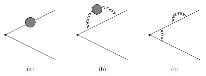
Figure 3: Two-loop heavy-quark self-energy diagrams with eikonal lines.

In this section we calculate the diagrams in Fig. 3 and their counterterms. We will denote by I3′I^{\prime}_{3} the diagrams shown in Fig. 3 and by I3c.t.I^{c.t.}_{3} their counterterms. The total contribution is then I3=I3′+I3c.t.I_{3}=I^{\prime}_{3}+I^{c.t.}_{3}. As for diagram 1(b) we introduce a regulator k′k^{\prime} in the quark momentum and then expand around vi⋅k′=0v_{i}\cdot k^{\prime}=0 at constant ϵ\epsilon. We also find it convient to define

Kβ=−ln⁡(1−β2)+5​ln⁡2+ln⁡π−γE−i​π.K_{\beta}=-\ln(1-\beta^{2})+5\ln 2+\ln\pi-\gamma_{E}-i\pi. (37)

IV.1 I3​aI_{3a}

Here we calculate the three diagrams represented by Fig. 3(a) which are shown in detail in Fig. 4. Note that an additional graph involving a three-gluon vertex with all three gluons attached to the same eikonal line vanishes.

Refer to caption
Figure 4: Detail of the diagrams of Fig. 3(a).

We begin with the diagram labeled (3a1i). Using Eq. (70) we find

I3​a​1​i′=αs2π2​{1ϵ2+1ϵ​Kβ}\displaystyle I^{\prime}_{3a1i}=\frac{\alpha_{s}^{2}}{\pi^{2}}\left\{\frac{1}{\epsilon^{2}}+\frac{1}{\epsilon}K_{\beta}\right\} (38)

with counterterm I3​a​1​ic.t.=(αs2/π2)[−2/ϵ2−Kβ/ϵ].I_{3a1i}^{c.t.}=(\alpha_{s}^{2}/\pi^{2})[-2/\epsilon^{2}-K_{\beta}/\epsilon]. Then

I3​a​1​i=αs2π2​(−1)ϵ2.I_{3a1i}=\frac{\alpha_{s}^{2}}{\pi^{2}}\frac{(-1)}{\epsilon^{2}}. (39)

Next we calculate I3​a​1​i​i′I^{\prime}_{3a1ii}. Using Eq. (73) we find

I3​a​1​i​i′=αs2π2​{12​ϵ2+12​ϵ​[1+Kβ]}I^{\prime}_{3a1ii}=\frac{\alpha_{s}^{2}}{\pi^{2}}\left\{\frac{1}{2\,\epsilon^{2}}+\frac{1}{2\,\epsilon}\left[1+K_{\beta}\right]\right\} (40)

with counterterm I3​a​1​i​ic.t.=(αs2/π2)[−1/ϵ2−Kβ/(2ϵ)].I_{3a1ii}^{c.t.}=(\alpha_{s}^{2}/\pi^{2})[-1/\epsilon^{2}-K_{\beta}/(2\epsilon)]. Then

I3​a​1​i​i=αs2π2​{−12​ϵ2+12​ϵ}.I_{3a1ii}=\frac{\alpha_{s}^{2}}{\pi^{2}}\left\{-\frac{1}{2\,\epsilon^{2}}+\frac{1}{2\,\epsilon}\right\}. (41)

Adding Eqs. (39) and (41) and denoting the sum by I3​a​1I_{3a1}, we find

I3​a​1=αs2π2​{−32​ϵ2+12​ϵ}.I_{3a1}=\frac{\alpha_{s}^{2}}{\pi^{2}}\left\{-\frac{3}{2\,\epsilon^{2}}+\frac{1}{2\,\epsilon}\right\}. (42)

Last we calculate I3​a​2′I^{\prime}_{3a2}, given by

I3​a​2′=gs4​∫dn​k1(2​π)n​dn​k2(2​π)n​viμvi⋅k′​viρvi⋅(k′−k1)\displaystyle\hskip-8.53581ptI^{\prime}_{3a2}=g_{s}^{4}\int\frac{d^{n}k_{1}}{(2\pi)^{n}}\frac{d^{n}k_{2}}{(2\pi)^{n}}\frac{v_{i}^{\mu}}{v_{i}\cdot k^{\prime}}\,\frac{v_{i}^{\rho}}{v_{i}\cdot(k^{\prime}-k_{1})}
×viνvi⋅(k′−k1−k2)​viσvi⋅(k′−k2)​(−i)​gμ​νk12​(−i)​gρ​σk22.\displaystyle\times\frac{v_{i}^{\nu}}{v_{i}\cdot(k^{\prime}-k_{1}-k_{2})}\,\frac{v_{i}^{\sigma}}{v_{i}\cdot(k^{\prime}-k_{2})}\frac{(-i)g_{\mu\nu}}{k_{1}^{2}}\frac{(-i)g_{\rho\sigma}}{k_{2}^{2}}\,.

Using Eqs. (74), (75), and (76), we find the UV poles of the integral

I3​a​2′=αs2π2​{−1ϵ2−1ϵ​[12+Kβ]}I^{\prime}_{3a2}=\frac{\alpha_{s}^{2}}{\pi^{2}}\left\{-\frac{1}{\epsilon^{2}}-\frac{1}{\epsilon}\left[\frac{1}{2}+K_{\beta}\right]\right\} (44)

with counterterm I3​a​2c.t.=(αs2/π2)​[2/ϵ2+Kβ/ϵ].I_{3a2}^{c.t.}=(\alpha_{s}^{2}/\pi^{2})[2/\epsilon^{2}+K_{\beta}/\epsilon]. Then

I3​a​2=αs2π2​{1ϵ2−12​ϵ}.I_{3a2}=\frac{\alpha_{s}^{2}}{\pi^{2}}\left\{\frac{1}{\epsilon^{2}}-\frac{1}{2\,\epsilon}\right\}. (45)

IV.2 I3​bI_{3b}

In this section we calculate the three self-energy diagrams (with quark, gluon, and ghost loops) represented by Fig. 3(b). Note that an additional diagram with a four-gluon vertex vanishes.

After several manipulations the quark-loop diagram becomes

I′3​b​q=−4nfgs4(2​π)2​n1vi⋅k′∫dn​k​dn​lk4​vi⋅(k−k′)​l2​(l−k)2\displaystyle\hskip-11.38109ptI^{\prime}_{3bq}=-4n_{f}\frac{g_{s}^{4}}{(2\pi)^{2n}}\frac{1}{v_{i}\cdot k^{\prime}}\int\frac{d^{n}k\,d^{n}l}{k^{4}\,v_{i}\cdot(k-k^{\prime})\,l^{2}\,(l-k)^{2}}
×[2​(vi⋅l)2−vi2​l2−2​vi⋅l​vi⋅k+vi2​l⋅k].\displaystyle\times\left[2(v_{i}\cdot l)^{2}-v_{i}^{2}\,l^{2}-2v_{i}\cdot l\,v_{i}\cdot k+v_{i}^{2}\,l\cdot k\right]\,. (46)

Expanding around vi⋅k′=0v_{i}\cdot k^{\prime}=0 this gives

I3​b​q′=4​nf​gs4(2​π)2​n​∫dn​kk4​(vi⋅k)2​∫dn​ll2​(l−k)2\displaystyle\hskip-31.29802ptI^{\prime}_{3bq}=4n_{f}\frac{g_{s}^{4}}{(2\pi)^{2n}}\int\frac{d^{n}k}{k^{4}\,(v_{i}\cdot k)^{2}}\int\frac{d^{n}l}{l^{2}\,(l-k)^{2}}
×[−vi2l⋅k−2(vi⋅l)2+2vi⋅lvi⋅k].\displaystyle\times\left[-v_{i}^{2}\,l\cdot k-2(v_{i}\cdot l)^{2}+2v_{i}\cdot l\,v_{i}\cdot k\right]\,. (47)

A calculation of the UV poles of the integral using Eq. (77) gives

I3​b​q′=αs2π2​nf3​{−1ϵ2−1ϵ​[56+Kβ]}I^{\prime}_{3bq}=\frac{\alpha_{s}^{2}}{\pi^{2}}\frac{n_{f}}{3}\left\{-\frac{1}{\epsilon^{2}}-\frac{1}{\epsilon}\left[\frac{5}{6}+K_{\beta}\right]\right\} (48)

with counterterm I3​b​qc.t.=(αs2/π2)​(nf/3)​[2/ϵ2+Kβ/ϵ]I_{3bq}^{c.t.}=(\alpha_{s}^{2}/\pi^{2})(n_{f}/3)[2/\epsilon^{2}+K_{\beta}/\epsilon]. Then

I3​b​q=αs2π2​nf3​[1ϵ2−56​ϵ].I_{3bq}=\frac{\alpha_{s}^{2}}{\pi^{2}}\frac{n_{f}}{3}\left[\frac{1}{\epsilon^{2}}-\frac{5}{6\,\epsilon}\right]. (49)

Next we calculate the gluon-loop self-energy diagram in Fig. 3(b) which, after several manipulations, becomes

I′3​b​g​l=−gs42​(2​π)2​n1vi⋅k′∫dn​kvi⋅(k−k′)\displaystyle\hskip-28.45274ptI^{\prime}_{3bgl}=-\frac{g_{s}^{4}}{2(2\pi)^{2n}}\frac{1}{v_{i}\cdot k^{\prime}}\int\frac{d^{n}k}{v_{i}\cdot(k-k^{\prime})}
×{[4​vi2k2+(n−6)(vi⋅k)2k4]∫dn​ll2​(k−l)2\displaystyle\times\left\{\left[\frac{4\,v_{i}^{2}}{k^{2}}+(n-6)\frac{(v_{i}\cdot k)^{2}}{k^{4}}\right]\int\frac{d^{n}l}{l^{2}(k-l)^{2}}\right.
−(4n−6)vi⋅kk4∫dnlvi⋅ll2​(k−l)2\displaystyle\quad\quad{}-(4n-6)\frac{v_{i}\cdot k}{k^{4}}\int d^{n}l\frac{v_{i}\cdot l}{l^{2}(k-l)^{2}}
+(4​n−6)k4∫dnl(vi⋅l)2l2​(k−l)2}.\displaystyle\quad\quad\left.{}+\frac{(4n-6)}{k^{4}}\int d^{n}l\frac{(v_{i}\cdot l)^{2}}{l^{2}(k-l)^{2}}\right\}. (50)

Expanding around vi⋅k′=0v_{i}\cdot k^{\prime}=0 this gives

I3​b​g​l′=−αs2π2​2−5+2​ϵ​i​π−2+3​ϵ2​(1−β2)\displaystyle\hskip-28.45274ptI^{\prime}_{3bgl}=-\frac{\alpha_{s}^{2}}{\pi^{2}}2^{-5+2\epsilon}i\pi^{-2+\frac{3\epsilon}{2}}(1-\beta^{2})
×Γ⁡(ϵ2)​[Γ⁡(1−ϵ2)]2​1Γ⁡(2−ϵ)\displaystyle\hskip-14.22636pt\times\Gamma\left(\frac{\epsilon}{2}\right)\left[\Gamma\left(1-\frac{\epsilon}{2}\right)\right]^{2}\frac{1}{\Gamma(2-\epsilon)}
×[2−(10−4​ϵ)8​13−ϵ]​∫dn​k(vi⋅k)2​(k2)1+ϵ2.\displaystyle\hskip-14.22636pt\times\left[2-\frac{(10-4\epsilon)}{8}\frac{1}{3-\epsilon}\right]\int\frac{d^{n}k}{(v_{i}\cdot k)^{2}\,(k^{2})^{1+\frac{\epsilon}{2}}}. (51)

Using Eq. (77) the UV poles of the integral are then

I3​b​g​l′=αs2π2​1948​{−1ϵ2−1ϵ​[5857+Kβ]}.I^{\prime}_{3bgl}=\frac{\alpha_{s}^{2}}{\pi^{2}}\frac{19}{48}\left\{-\frac{1}{\epsilon^{2}}-\frac{1}{\epsilon}\left[\frac{58}{57}+K_{\beta}\right]\right\}. (52)

The counterterm is I3​b​g​lc.t.=(αs2/π2)​(19/48)​[2/ϵ2+Kβ/ϵ].I_{3bgl}^{c.t.}=(\alpha_{s}^{2}/\pi^{2})(19/48)[2/\epsilon^{2}+K_{\beta}/\epsilon]. Then

I3​b​g​l=αs2π2​1948​{1ϵ2−5857​ϵ}.I_{3bgl}=\frac{\alpha_{s}^{2}}{\pi^{2}}\frac{19}{48}\left\{\frac{1}{\epsilon^{2}}-\frac{58}{57\,\epsilon}\right\}. (53)

Last we calculate the ghost-loop self-energy diagram in Fig. 3(b). After several manipulations and expanding around vi⋅k′=0v_{i}\cdot k^{\prime}=0 this gives

I3​b​g​h′=αs2π2​2−6+2​ϵ​π−2+3​ϵ2​i​(1−β2)​Γ​(−1+ϵ2)\displaystyle\hskip-22.76219ptI^{\prime}_{3bgh}=\frac{\alpha_{s}^{2}}{\pi^{2}}2^{-6+2\epsilon}\pi^{-2+\frac{3\epsilon}{2}}i(1-\beta^{2})\Gamma\left(-1+\frac{\epsilon}{2}\right)
×[Γ⁡(2−ϵ2)]2​1Γ⁡(4−ϵ)​∫dn​k(vi⋅k)2​(k2)1+ϵ2.\displaystyle\hskip-8.53581pt\times\left[\Gamma\left(2-\frac{\epsilon}{2}\right)\right]^{2}\frac{1}{\Gamma(4-\epsilon)}\int\frac{d^{n}k}{(v_{i}\cdot k)^{2}\,(k^{2})^{1+\frac{\epsilon}{2}}}. (54)

Using Eq. (77) the UV poles are then given by

I3​b​g​h′=αs2π2​148​{−1ϵ2−1ϵ​[43+Kβ]}I^{\prime}_{3bgh}=\frac{\alpha_{s}^{2}}{\pi^{2}}\frac{1}{48}\left\{-\frac{1}{\epsilon^{2}}-\frac{1}{\epsilon}\left[\frac{4}{3}+K_{\beta}\right]\right\} (55)

with counterterm I3​b​g​hc.t.=(αs2/π2)​(1/48)​[2/ϵ2+Kβ/ϵ].I_{3bgh}^{c.t.}=(\alpha_{s}^{2}/\pi^{2})(1/48)[2/\epsilon^{2}+K_{\beta}/\epsilon]. Then

I3​b​g​h=αs2π2​148​{1ϵ2−43​ϵ}.I_{3bgh}=\frac{\alpha_{s}^{2}}{\pi^{2}}\frac{1}{48}\left\{\frac{1}{\epsilon^{2}}-\frac{4}{3\,\epsilon}\right\}. (56)

The sum of the gluon and ghost loops, Eqs. (53) and (56), denoted by I3​b​gI_{3bg}, is then

I3​b​g=αs2π2​512​[1ϵ2−3130​ϵ].I_{3bg}=\frac{\alpha_{s}^{2}}{\pi^{2}}\frac{5}{12}\left[\frac{1}{\epsilon^{2}}-\frac{31}{30\,\epsilon}\right]. (57)

IV.3 I3​cI_{3c}

Finally we calculate the diagram in Fig. 3(c). Using Eqs. (Appendix) and (70) and adding the one-loop counterterm, we find

I3​c=αs2π2​(1+β2)2​β​(−1)ϵ2​ln⁡(1−β1+β).I_{3c}=\frac{\alpha_{s}^{2}}{\pi^{2}}\frac{(1+\beta^{2})}{2\beta}\frac{(-1)}{\epsilon^{2}}\ln\left(\frac{1-\beta}{1+\beta}\right). (58)

V Two-loop soft anomalous dimension

We now combine the kinematic results from sections 3 and 4 with color and symmetry factors. The contribution of the diagrams in Figs. (2) and (3) to the two-loop soft anomalous dimension is

CF2​[I2​a+I2​b+2​I2​d+2​I2​e+I3​a​1+I3​a​2+I3​c]\displaystyle C_{F}^{2}\left[I_{2a}+I_{2b}+2\,I_{2d}+2\,I_{2e}+I_{3a1}+I_{3a2}+I_{3c}\right]
+CF​CA​[−12​I2​b+I2​f−I2​c​g−I2​e−I3​b​g−12​I3​a​2]\displaystyle\hskip-8.53581pt{}+C_{F}\,C_{A}\left[-\frac{1}{2}I_{2b}+I_{2f}-I_{2cg}-I_{2e}-I_{3bg}-\frac{1}{2}I_{3a2}\right]
+12​CF​[I2​c​q+I3​b​q]\displaystyle\hskip-8.53581pt{}+\frac{1}{2}C_{F}\left[I_{2cq}+I_{3bq}\right]
=αs2π2​[−12​ϵ2​(ΓS(1))2+β04​ϵ2​ΓS(1)−12​ϵ​ΓS(2)].\displaystyle\hskip-8.53581pt=\frac{\alpha_{s}^{2}}{\pi^{2}}\left[-\frac{1}{2\epsilon^{2}}\left(\Gamma_{S}^{(1)}\right)^{2}+\frac{\beta_{0}}{4\epsilon^{2}}\Gamma_{S}^{(1)}-\frac{1}{2\epsilon}\Gamma_{S}^{(2)}\right]. (59)

On the right-hand side of Eq. (59) in addition to ΓS(2)\Gamma_{S}^{(2)}, which appears in the coefficient of the 1/ϵ1/\epsilon pole, there also appear terms from the exponentiation of the one-loop result and the running of the coupling, with β0=(11/3)​CA−2​nf/3\beta_{0}=(11/3)C_{A}-2n_{f}/3, CA=NcC_{A}=N_{c}, which account for all the double poles of the graphs. From Eq. (59) we solve for the two-loop soft anomalous dimension:

ΓS(2)=K2ΓS(1)+CFCA{12+ζ22+12ln2(1−β1+β)\displaystyle\hskip-14.22636pt\Gamma_{S}^{(2)}=\frac{K}{2}\,\Gamma_{S}^{(1)}+C_{F}C_{A}\left\{\frac{1}{2}+\frac{\zeta_{2}}{2}+\frac{1}{2}\ln^{2}\left(\frac{1-\beta}{1+\beta}\right)\right.
−(1+β2)28​β2[ζ3+ζ2ln(1−β1+β)+13ln3(1−β1+β)\displaystyle\hskip-14.22636pt{}-\frac{(1+\beta^{2})^{2}}{8\beta^{2}}\left[\zeta_{3}+\zeta_{2}\ln\left(\frac{1-\beta}{1+\beta}\right)+\frac{1}{3}\ln^{3}\left(\frac{1-\beta}{1+\beta}\right)\right.
+ln(1−β1+β)Li2((1−β)2(1+β)2)−Li3((1−β)2(1+β)2)]\displaystyle\hskip-8.53581pt\left.{}+\ln\left(\frac{1-\beta}{1+\beta}\right){\rm Li}_{2}\left(\frac{(1-\beta)^{2}}{(1+\beta)^{2}}\right)-{\rm Li}_{3}\left(\frac{(1-\beta)^{2}}{(1+\beta)^{2}}\right)\right]
−(1+β2)4​β[ζ2−ζ2ln(1−β1+β)+ln2(1−β1+β)\displaystyle\hskip-14.22636pt{}-\frac{(1+\beta^{2})}{4\beta}\left[\zeta_{2}-\zeta_{2}\ln\left(\frac{1-\beta}{1+\beta}\right)+\ln^{2}\left(\frac{1-\beta}{1+\beta}\right)\right.
−13​ln3⁡(1−β1+β)+2​ln⁡(1−β1+β)​ln⁡((1+β)24​β)\displaystyle{}-\frac{1}{3}\ln^{3}\left(\frac{1-\beta}{1+\beta}\right)+2\ln\left(\frac{1-\beta}{1+\beta}\right)\ln\left(\frac{(1+\beta)^{2}}{4\beta}\right)
−Li2((1−β)2(1+β)2)]}\displaystyle\hskip 42.67912pt\left.\left.{}-{\rm Li}_{2}\left(\frac{(1-\beta)^{2}}{(1+\beta)^{2}}\right)\right]\right\} (60)

where

K=CA​(6718−ζ2)−5​nf9.K=C_{A}\left(\frac{67}{18}-\zeta_{2}\right)-\frac{5n_{f}}{9}. (61)

A slightly different but equivalent expression is given in Ref. [3].

In terms of the cusp angle γ\gamma we find

ΓS(2)=K2ΓS(1)+CFCA{12+ζ22+γ22−12coth2γ\displaystyle\hskip-14.22636pt\Gamma_{S}^{(2)}=\frac{K}{2}\,\Gamma_{S}^{(1)}+C_{F}C_{A}\left\{\frac{1}{2}+\frac{\zeta_{2}}{2}+\frac{\gamma^{2}}{2}-\frac{1}{2}\coth^{2}\gamma\right.
×[ζ3−ζ2​γ−γ33−γ​Li2​(e−2​γ)−Li3​(e−2​γ)]\displaystyle\quad\times\left[\zeta_{3}-\zeta_{2}\gamma-\frac{\gamma^{3}}{3}-\gamma\,{\rm Li}_{2}\left(e^{-2\gamma}\right)-{\rm Li}_{3}\left(e^{-2\gamma}\right)\right]
−12cothγ[ζ2+ζ2γ+γ2+γ33\displaystyle\hskip-11.38109pt{}-\frac{1}{2}\coth\gamma\left[\zeta_{2}+\zeta_{2}\gamma+\gamma^{2}+\frac{\gamma^{3}}{3}\right.
+2γln(1−e−2​γ)−Li2(e−2​γ)]}.\displaystyle\hskip 39.83385pt\left.\left.{}+2\,\gamma\,\ln\left(1-e^{-2\gamma}\right)-{\rm Li}_{2}\left(e^{-2\gamma}\right)\right]\right\}. (62)

This expression is consistent with the form of the two-loop cusp anomalous dimension given in Ref. [5] (which involves a few uncalculated integrals), and it is also consistent with the two-loop heavy-quark form factor of Ref. [6].

Using the above results we can find the soft-gluon logarithms in the cross section for e+​e−→t​t¯e^{+}e^{-}\rightarrow t{\bar{t}}, which are of the form lnn−1⁡(β2)/β2\ln^{n-1}(\beta^{2})/\beta^{2} at nn-th order in αs\alpha_{s}. The first-order soft-gluon corrections are σ(1)=σB​(αs/π)​ 2​ΓS(1)/β2\sigma^{(1)}=\sigma^{B}\,(\alpha_{s}/\pi)\,2\,\Gamma_{S}^{(1)}/\beta^{2} with σB\sigma^{B} the Born cross section. The second-order soft-gluon corrections are

σ(2)=σBαs2π2{[4(ΓS(1))2−β0ΓS(1)]ln⁡(β2)β2\displaystyle\hskip-22.76219pt\sigma^{(2)}=\sigma^{B}\frac{\alpha_{s}^{2}}{\pi^{2}}\left\{\left[4(\Gamma_{S}^{(1)})^{2}-\beta_{0}\,\Gamma_{S}^{(1)}\right]\frac{\ln(\beta^{2})}{\beta^{2}}\right.
+[2T1ΓS(1)+2ΓS(2)]1β2}\displaystyle\hskip 42.67912pt\left.{}+\left[2\,T_{1}\,\Gamma_{S}^{(1)}+2\,\Gamma_{S}^{(2)}\right]\frac{1}{\beta^{2}}\right\} (63)

with T1T_{1} the NLO virtual corrections.

Refer to caption
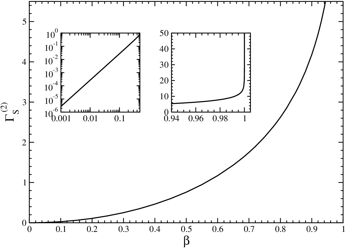
Figure 5: The two-loop soft anomalous dimension ΓS(2)\Gamma_{S}^{(2)}.

In Figure 5 we plot ΓS(2)\Gamma_{S}^{(2)} versus β\beta. The insets show the small and large β\beta regions in detail. Note that both ΓS(1)\Gamma_{S}^{(1)} and ΓS(2)\Gamma_{S}^{(2)} vanish in the threshold limit, β=0\beta=0, and they both diverge in the massless limit, β=1\beta=1.

The small-β\beta expansion of Eq. (60) is

ΓS​exp(2)\displaystyle\Gamma_{S\,\rm exp}^{(2)} =\displaystyle= −227​β2​[CF​CA​(18​ζ2−47)+5​nf​CF]\displaystyle-\frac{2}{27}\beta^{2}\left[C_{F}C_{A}(18\zeta_{2}-47)+5n_{f}C_{F}\right] (64)
+𝒪⁡(β4).\displaystyle\hskip 85.35826pt{}+{\cal O}(\beta^{4})\,.

ΓS(2)\Gamma_{S}^{(2)} is an even function of β\beta and hence only even powers of β\beta appear in the expansion. As shown in [3] the expansion provides a good approximation to the complete result for small β\beta.

Next we study the large-β\beta behavior of ΓS(2)\Gamma_{S}^{(2)}, Eq. (60). As β→1\beta\rightarrow 1,

ΓS(2)→K2​ΓS(1)+CF​CA​(1−ζ3)2\Gamma_{S}^{(2)}\rightarrow\frac{K}{2}\Gamma_{S}^{(1)}+C_{F}C_{A}\frac{(1-\zeta_{3})}{2} (65)

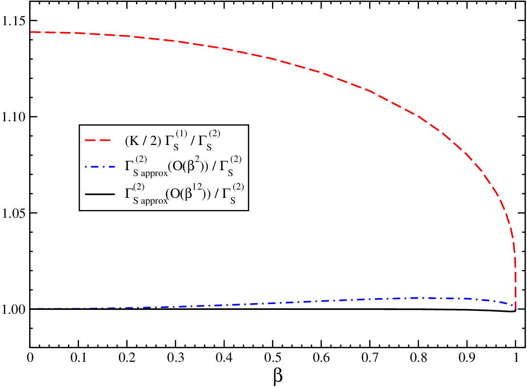
with ΓS(1)=CF​[ln⁡(2​vi⋅vj/vi2​vj2)−1]\Gamma_{S}^{(1)}=C_{F}\left[\ln\left(2v_{i}\cdot v_{j}/\sqrt{v_{i}^{2}v_{j}^{2}}\right)-1\right]. Since ΓS(1)\Gamma_{S}^{(1)} diverges at β=1\beta=1, ΓS(2)≈(K/2)​ΓS(1)\Gamma_{S}^{(2)}\approx(K/2)\Gamma_{S}^{(1)} at that limit. This is consistent with the massless case ΓS(2)=K2​ΓS(1)\Gamma_{S}^{(2)}=\frac{K}{2}\Gamma_{S}^{(1)} with ΓS(1)=CF​ln⁡(vi⋅vj)\Gamma_{S}^{(1)}=C_{F}\ln(v_{i}\cdot v_{j}) [7, 8, 9]. As is clear from Eq. (60) the massive case is much more complicated than the simple massless relation, and (K/2)​ΓS(1)(K/2)\Gamma_{S}^{(1)} is just the first of many terms in the expression for ΓS(2)\Gamma_{S}^{(2)}. Figure 6 shows that numerically the ratio (K/2)​ΓS(1)/ΓS(2)(K/2)\Gamma_{S}^{(1)}/\Gamma_{S}^{(2)} goes to 1 as β→1\beta\rightarrow 1, the massless limit, as expected from the above discussion, but it is significantly different from 1 at other β\beta and takes the value 1.144 at the other end of the range, β=0\beta=0.

In the mixed massive-massless case, with viv_{i} the heavy quark and vjv_{j} the massless quark, we find

ΓS(2)=K2​ΓS(1)+CF​CA​(1−ζ3)4\Gamma_{S}^{(2)}=\frac{K}{2}\Gamma_{S}^{(1)}+C_{F}C_{A}\frac{(1-\zeta_{3})}{4} (66)

with

ΓS(1)=CF​[ln⁡(2​vi⋅vjvi2)−12].\Gamma_{S}^{(1)}=C_{F}\left[\ln\left(\frac{\sqrt{2}\,v_{i}\cdot v_{j}}{\sqrt{v_{i}^{2}}}\right)-\frac{1}{2}\right]. (67)

Given that the small-β\beta expansion gives very good approximations to ΓS(2)\Gamma_{S}^{(2)} at smaller β\beta while the expression (K/2)​ΓS(1)(K/2)\,\Gamma_{S}^{(1)} is the large-β\beta limit, we can derive an approximation to ΓS(2)\Gamma_{S}^{(2)}, Eq. (60), valid for all β\beta using the following approximate formula:

ΓS​approx(2)=ΓS​exp(2)+K2​ΓS(1)−K2​ΓS​exp(1)\displaystyle\hskip-28.45274pt\Gamma^{(2)}_{S\,\rm approx}=\Gamma^{(2)}_{S\,\rm exp}+\frac{K}{2}\Gamma_{S}^{(1)}-\frac{K}{2}\Gamma^{(1)}_{S\,\rm exp}
=K2​ΓS(1)+CF​CA​(1−23​ζ2)​β2+𝒪⁡(β4).\displaystyle\hskip-8.53581pt=\frac{K}{2}\Gamma_{S}^{(1)}+C_{F}C_{A}\left(1-\frac{2}{3}\zeta_{2}\right)\beta^{2}+{\cal O}\left(\beta^{4}\right). (68)
Refer to caption
Figure 6: Approximations to ΓS(2)\Gamma_{S}^{(2)}.

As seen from Fig. 6, adding just the β2\beta^{2} terms to (K/2)​ΓS(1)(K/2)\,\Gamma_{S}^{(1)} provides an excellent approximation to the exact result for for all β\beta. If we keep additional terms through order β12\beta^{12} then the approximation is extremely good and does not differ by more than one per mille anywhere in the β\beta range.

Finally we discuss extensions to single top [10, 11] and top pair [10, 12] production at hadron colliders. As first shown in Ref. [3], since the two-loop soft anomalous dimensions for single top and top pair processes involve eikonal graphs with both massless and massive eikonal lines, it is clear that the simple massless relation ΓS(2)=(K/2)​ΓS(1)\Gamma_{S}^{(2)}=(K/2)\,\Gamma_{S}^{(1)} will not hold. This observation was also made later in Refs. [13, 14]. The two-loop soft anomalous dimension ΓS(2)\Gamma_{S}^{(2)} derived in [3] and in this paper is an essential ingredient for next-to-next-to-leading logarithm (NNLL) resummation for heavy quark hadroproduction and has been used in very recent calculations [14, 15, 16, 17].

Acknowledgements.
This work was supported by the National Science Foundation under Grant No. PHY 0855421.

Appendix

We list results for the UV poles of several of the many integrals needed in the calculation of the two-loop soft anomalous dimension.

∫dn​kk2​vi⋅k​vj⋅k=iϵ​(−1)−1−ϵ2​π2−ϵ2​23+3​ϵ2\displaystyle\hskip-19.91692pt\int\frac{d^{n}k}{k^{2}\,v_{i}\cdot k\,v_{j}\cdot k}=\frac{i}{\epsilon}(-1)^{-1-\frac{\epsilon}{2}}\pi^{2-\frac{\epsilon}{2}}2^{3+3\frac{\epsilon}{2}}
×Γ⁡(1+ϵ2)​F12​(12,1+ϵ2,32,β2)\displaystyle\quad\times\Gamma\left(1+\frac{\epsilon}{2}\right)\,{}_{2}F_{1}\left(\frac{1}{2},1+\frac{\epsilon}{2};\frac{3}{2};\beta^{2}\right)
=i​4​π2β{1ϵln(1−β1+β)\displaystyle=\frac{i4\pi^{2}}{\beta}\left\{\frac{1}{\epsilon}\ln\left(\frac{1-\beta}{1+\beta}\right)\right.
+12​(2​ln⁡2−ln⁡π−γE−i​π)​ln⁡(1−β1+β)\displaystyle\quad{}+\frac{1}{2}(2\ln 2-\ln\pi-\gamma_{E}-i\pi)\ln\left(\frac{1-\beta}{1+\beta}\right)
+14​ln2⁡(1+β)−14​ln2⁡(1−β)\displaystyle\quad{}+\frac{1}{4}\ln^{2}(1+\beta)-\frac{1}{4}\ln^{2}(1-\beta)
−12Li2(1+β2)+12Li2(1−β2)}+𝒪(ϵ)\displaystyle\quad\left.{}-\frac{1}{2}{\rm Li}_{2}\left(\frac{1+\beta}{2}\right)+\frac{1}{2}{\rm Li}_{2}\left(\frac{1-\beta}{2}\right)\right\}+{\cal O}(\epsilon)

where F12{}_{2}F_{1} is the Gauss hypergeometric function.

∫dn​kk2​(vi⋅k)2=iϵ​(−1)1−ϵ2​π2−ϵ2​ 23+3​ϵ2\displaystyle\hskip-25.60747pt\int\frac{d^{n}k}{k^{2}\,(v_{i}\cdot k)^{2}}=\frac{i}{\epsilon}\,(-1)^{1-\frac{\epsilon}{2}}\,\pi^{2-\frac{\epsilon}{2}}\,2^{3+3\frac{\epsilon}{2}}
×(1−β2)−1−ϵ2​Γ​(1+ϵ2)\displaystyle\quad\quad\times(1-\beta^{2})^{-1-\frac{\epsilon}{2}}\Gamma\left(1+\frac{\epsilon}{2}\right)
=−i​8​π21−β2[1ϵ−12ln(1−β2)\displaystyle\hskip-22.76219pt=-\frac{i8\pi^{2}}{1-\beta^{2}}\left[\frac{1}{\epsilon}-\frac{1}{2}\ln(1-\beta^{2})\right.
+32ln2−12lnπ−γE2−i​π2]+𝒪(ϵ).\displaystyle\hskip 19.91692pt\left.{}+\frac{3}{2}\ln 2-\frac{1}{2}\ln\pi-\frac{\gamma_{E}}{2}-\frac{i\pi}{2}\right]+{\cal O}(\epsilon). (70)
∫dn​k(k2)1+ϵ2​vi⋅k​vj⋅k=iϵ2​(−1)1−ϵβ​ 22​ϵ\displaystyle\hskip-25.60747pt\int\frac{d^{n}k}{(k^{2})^{1+\frac{\epsilon}{2}}\,v_{i}\cdot k\,v_{j}\cdot k}=\frac{i}{\epsilon^{2}}\,\frac{(-1)^{1-\epsilon}}{\beta}\,2^{2\epsilon}
×π2−ϵ2​Γ​(1+ϵ)​1Γ⁡(1+ϵ2)\displaystyle\hskip-11.38109pt\times\pi^{2-\frac{\epsilon}{2}}\,\Gamma(1+\epsilon)\frac{1}{\Gamma\left(1+\frac{\epsilon}{2}\right)}
×[(1−β)−ϵF12(−ϵ,1+ϵ;1−ϵ;1−β2)\displaystyle\hskip-11.38109pt\times\left[(1-\beta)^{-\epsilon}{}_{2}F_{1}\left(-\epsilon,1+\epsilon;1-\epsilon;\frac{1-\beta}{2}\right)\right.
−(1+β)−ϵF12(−ϵ,1+ϵ;1−ϵ;1+β2)].\displaystyle\hskip-5.69054pt\left.{}-(1+\beta)^{-\epsilon}{}_{2}F_{1}\left(-\epsilon,1+\epsilon;1-\epsilon;\frac{1+\beta}{2}\right)\right]. (71)
∫dn​kk2​(vi⋅k)1+ϵ​vj⋅k=i​π2−ϵ2ϵ⁡(1+ϵ)​22+9​ϵ2​(−1)−1−3​ϵ2\displaystyle\hskip-25.60747pt\int\frac{d^{n}k}{k^{2}\,(v_{i}\cdot k)^{1+\epsilon}\,v_{j}\cdot k}=\frac{i\pi^{2-\frac{\epsilon}{2}}}{\epsilon(1+\epsilon)}2^{2+\frac{9\epsilon}{2}}(-1)^{-1-\frac{3\epsilon}{2}}
×(1−β2)−1−3​ϵ2​Γ​(1+3​ϵ2)​1Γ⁡(1+ϵ)\displaystyle\hskip-17.07164pt\times(1-\beta^{2})^{-1-\frac{3\epsilon}{2}}\,\Gamma\left(1+\frac{3\epsilon}{2}\right)\frac{1}{\Gamma(1+\epsilon)}
×F1​[1+ϵ;1+3​ϵ2,1+3​ϵ2;2+ϵ;2​β1+β,−2​β1−β]\displaystyle\hskip-17.07164pt\times F_{1}[1+\epsilon;1+\frac{3\epsilon}{2},1+\frac{3\epsilon}{2};2+\epsilon;\frac{2\beta}{1+\beta},\frac{-2\beta}{1-\beta}] (72)

where F1F_{1} is the Appell hypergeometric function.

∫dn​k2k22​[vi⋅(k1+k2)]2=iϵ​(−1)−1+ϵ2(1+ϵ)​ 24−ϵ2​π3−ϵ2\displaystyle\hskip-19.91692pt\int\frac{d^{n}k_{2}}{k_{2}^{2}\,\left[v_{i}\cdot(k_{1}+k_{2})\right]^{2}}=\frac{i}{\epsilon}\,\frac{(-1)^{-1+\frac{\epsilon}{2}}}{(1+\epsilon)}\,2^{4-\frac{\epsilon}{2}}\,\pi^{\frac{3-\epsilon}{2}}
×(1−β2)−1+ϵ2​(vi⋅k1)−ϵ​Γ​(1+ϵ2)\displaystyle\quad\times(1-\beta^{2})^{-1+\frac{\epsilon}{2}}\,(v_{i}\cdot k_{1})^{-\epsilon}\,\Gamma\left(1+\frac{\epsilon}{2}\right)
×Γ⁡(1−ϵ2)​Γ​(3+ϵ2).\displaystyle\quad\times\Gamma\left(1-\frac{\epsilon}{2}\right)\,\Gamma\left(\frac{3+\epsilon}{2}\right)\,. (73)
∫dn​kk2​(vi⋅k)2+ϵ=i​π2−ϵ2ϵ⁡(1+ϵ)​22+9​ϵ2​(−1)−1−3​ϵ2\displaystyle\hskip-19.91692pt\int\frac{d^{n}k}{k^{2}\,(v_{i}\cdot k)^{2+\epsilon}}=\frac{i\pi^{2-\frac{\epsilon}{2}}}{\epsilon(1+\epsilon)}2^{2+\frac{9\epsilon}{2}}(-1)^{-1-\frac{3\epsilon}{2}}
×(1−β2)−1−3​ϵ2​Γ​(1+3​ϵ2)​1Γ⁡(1+ϵ).\displaystyle\quad\times(1-\beta^{2})^{-1-\frac{3\epsilon}{2}}\,\Gamma\left(1+\frac{3\epsilon}{2}\right)\frac{1}{\Gamma(1+\epsilon)}\,. (74)
∫dn​k1k12​vi⋅k1​vi⋅(k1+k2)=iϵ​(−1)ϵ2​ 22−ϵ2​π3−ϵ2\displaystyle\hskip-19.91692pt\int\frac{d^{n}k_{1}}{k_{1}^{2}\,v_{i}\cdot k_{1}\,v_{i}\cdot(k_{1}+k_{2})}=\frac{i}{\epsilon}\,(-1)^{\frac{\epsilon}{2}}\,2^{2-\frac{\epsilon}{2}}\,\pi^{\frac{3-\epsilon}{2}}
×(vi⋅k2)−ϵ​(1−β2)−1+ϵ2​Γ​(1+ϵ2)\displaystyle\quad\quad\times(v_{i}\cdot k_{2})^{-\epsilon}\,(1-\beta^{2})^{-1+\frac{\epsilon}{2}}\,\Gamma\left(1+\frac{\epsilon}{2}\right)
×Γ⁡(1−ϵ2)​Γ​(ϵ−12).\displaystyle\quad\quad\times\Gamma\left(1-\frac{\epsilon}{2}\right)\,\Gamma\left(\frac{\epsilon-1}{2}\right)\,. (75)
∫dn​k2k22​vi⋅k2​[vi⋅(k1+k2)]2=i1−ϵ​(−1)1+ϵ2\displaystyle\hskip-19.91692pt\int\frac{d^{n}k_{2}}{k_{2}^{2}\,v_{i}\cdot k_{2}\,[v_{i}\cdot(k_{1}+k_{2})]^{2}}=\frac{i}{1-\epsilon}\,(-1)^{1+\frac{\epsilon}{2}}
×23−3​ϵ2​π2−ϵ2​(vi⋅k1)−1−ϵ​(1−β2)−1+ϵ2\displaystyle\quad\times 2^{3-\frac{3\epsilon}{2}}\,\pi^{2-\frac{\epsilon}{2}}\,(v_{i}\cdot k_{1})^{-1-\epsilon}\,(1-\beta^{2})^{-1+\frac{\epsilon}{2}}
×Γ⁡(1−ϵ2)​Γ​(1+ϵ).\displaystyle\quad\times\Gamma\left(1-\frac{\epsilon}{2}\right)\,\Gamma(1+\epsilon)\,. (76)
∫dn​k(k2)1+ϵ2​(vi⋅k)2=iϵ​(−1)−1−ϵ​ 22+3​ϵ​π2−ϵ2\displaystyle\hskip-19.91692pt\int\frac{d^{n}k}{(k^{2})^{1+\frac{\epsilon}{2}}\,(v_{i}\cdot k)^{2}}=\frac{i}{\epsilon}\,(-1)^{-1-\epsilon}\,2^{2+3\epsilon}\,\pi^{2-\frac{\epsilon}{2}}
×(1−β2)−1−ϵ​Γ​(1+ϵ)​1Γ⁡(1+ϵ2).\displaystyle\quad\quad\times(1-\beta^{2})^{-1-\epsilon}\,\Gamma(1+\epsilon)\,\frac{1}{\Gamma\left(1+\frac{\epsilon}{2}\right)}\,. (77)

References

  • [1] N. Kidonakis, Phys. Rev. D 73, 034001 (2006) [hep-ph/0509079]; D 77, 053008 (2008), arXiv:0711.0142 [hep-ph]; Mod. Phys. Lett. A 19, 405 (2004) [hep-ph/0401147].
  • [2] N. Kidonakis and G. Sterman, Phys. Lett. B 387, 867 (1996); Nucl. Phys. B505, 321 (1997) [hep-ph/9705234]; N. Kidonakis, G. Oderda, and G. Sterman, Nucl. Phys. B531, 365 (1998) [hep-ph/9803241].
  • [3] N. Kidonakis, Phys. Rev. Lett. 102, 232003 (2009), arXiv:0903.2561 [hep-ph].
  • [4] S.V. Ivanov, G.P. Korchemsky, and A.V. Radyushkin, Yad. Fiz. 44, 230 (1986) [Sov. J. Nucl. Phys. 44, 145 (1986)].
  • [5] G.P. Korchemsky, A.V. Radyushkin, Phys. Lett. B 171, 459 (1986); Nucl. Phys. B283, 342 (1987); Phys. Lett. B 279, 359 (1992) [hep-ph/9203222].
  • [6] W. Bernreuther, R. Bonciani, T. Gehrmann, R. Heinesch, T. Leineweber, P. Mastrolia, and E. Remiddi, Nucl. Phys. B706, 245 (2005) [hep-ph/0406046].
  • [7] S.M. Aybat, L.J. Dixon, and G. Sterman, Phys. Rev. D 74, 074004 (2006) [hep-ph/0607309].
  • [8] T. Becher and M. Neubert, Phys. Rev. Lett. 102, 162001 (2009), arXiv:0901.0722 [hep-ph].
  • [9] E. Gardi and L. Magnea, JHEP 03, 079 (2009), arXiv:0901.1091 [hep-ph].
  • [10] N. Kidonakis, in these proceedings, arXiv:0909.0037 [hep-ph].
  • [11] N. Kidonakis, Phys. Rev. D 74, 114012 (2006) [hep-ph/0609287]; Phys. Rev. D 75, 071501 (2007) [hep-ph/0701080].
  • [12] N. Kidonakis and R. Vogt, Phys. Rev. D 68, 114014 (2003) [hep-ph/0308222]; Phys. Rev. D 78, 074005 (2008), arXiv:0805.3844 [hep-ph].
  • [13] A. Mitov, G. Sterman, and I. Sung, Phys. Rev. D 79, 094015 (2009), arXiv:0903.3241 [hep-ph].
  • [14] T. Becher and M. Neubert, Phys. Rev. D 79, 125004 (2009), arXiv:0904.1021 [hep-ph].
  • [15] M. Beneke, P. Falgari, and C. Schwinn, arXiv:0907.1443 [hep-ph].
  • [16] M. Czakon, A. Mitov, and G. Sterman, arXiv:0907.1790 [hep-ph].
  • [17] A. Ferroglia, M. Neubert, B.D. Pecjak, and L.L. Yang, arXiv:0907.4791 [hep-ph]; arXiv:0908.3676 [hep-ph].