SACLAY-T09/158
SISSA–64/2009/EP
Flavour violation in supersymmetric SO(10)
unification with a type II seesaw mechanism
Abstract
We study flavour violation in a supersymmetric SO(10) implementation of the type II seesaw mechanism, which provides a predictive realization of triplet leptogenesis. The experimental upper bounds on lepton flavour violating processes have a significant impact on the leptogenesis dynamics, in particular they exclude the strong washout regime. Requiring successful leptogenesis then constrains the otherwise largely unknown overall size of flavour-violating observables, thus yielding testable predictions. In particular, the branching ratio for lies within the reach of the MEG experiment if the superpartner spectrum is accessible at the LHC, and the supersymmetric contribution to can account for a significant part of the experimental value. We show that this scenario can be realized in a consistent SO(10) model achieving gauge symmetry breaking and doublet-triplet splitting in agreement with the proton decay bounds, improving on the MSSM prediction for , and reproducing the measured quark and lepton masses.
1 Introduction
Neutrino masses presumably arise at a scale much larger than the electroweak scale. If this is the case, a model-independent effective description of neutrino masses is possible at lower scales in terms of the dimension 5 operator [1], where is the -th family lepton doublet, is the Higgs doublet and is the scale at which the operator is generated, which can be as large as . While this effective description is essentially unique, the high-energy mechanism leading to the above dimension 5 operator is not. Generally, it is assumed to arise from the tree-level exchange of SM singlet fermions (type I seesaw mechanism [2]). In this case, the low-energy information from lepton masses and mixing only determines 9 out of the 18 high-energy seesaw parameters. Due to this arbitrariness, it is not possible to make definite predictions for the lepton asymmetry generated in the decays of the heavy singlet neutrinos [3], nor, in supersymmetric models, for the lepton flavour violating (LFV) effects induced by their Yukawa interactions [4].
On the other hand, the exchange of singlet fermions is not the only possible origin of the operator. In this paper, we consider the exchange of an SU(2)L triplet scalar with (type II or triplet seesaw mechanism [5]). More precisely, we consider the SO(10) [6] implementation of the triplet seesaw mechanism proposed in Ref. [7], in which all flavour parameters contributing to low-energy observables are determined in terms of the SM fermion masses and mixings11 1 Actually, the higher-dimensional operators needed to account for the measured masses of down quarks and charged leptons may affect this relation between high-energy and low-energy flavour parameters. We argue in Section 3.3 that the impact of this on physical observables is generally small, and neglect it in the following.. This allows to make testable predictions for these observables, up to a few unknown flavour-blind parameters. Particularly interesting is the possibility [7] of accounting for the baryon asymmetry of the universe via triplet leptogenesis. In usual type II models, it is necessary to introduce additional triplets or singlets in order to provide a rich enough flavour structure to induce a non-vanishing CP asymmetry in triplet decays [8]. This brings back into the game a number of flavour unknowns. On the contrary, in the scenario that we consider, the additional states are heavy quarks and leptons whose masses and couplings are determined in terms of low-energy parameters through SO(10) relations. The generated baryon asymmetry then directly depends on the light neutrino parameters.
In this paper, we pursue the exploration of this scenario by studying the flavour- and CP-violating effects induced by the couplings of the heavy states to the MSSM squarks and sleptons. Assuming flavour-universal soft supersymmetry breaking terms at the GUT scale, flavour-violating observables are predicted up to a few unknown scale parameters and to a mild model-dependent uncertainty, thus allowing to test the scenario. Besides the contributions of the type II seesaw triplet and of its SU(5) partners already studied in Ref. [9], the presence of heavy quarks and leptons gives rise to additional contributions to the slepton and squark soft terms. In particular, they induce flavour and CP violation in the slepton singlet and squark doublet sectors, which were absent in the SU(5) type II seesaw model.
The paper is organized as follows. In Section 2, we present the main features of the SO(10) scenario we consider. Section 3 contains a qualitative discussion of its predictions for flavour and CP violation. Model-building aspects including gauge coupling unification, doublet-triplet splitting and proton decay are briefly discussed in Section 4, and addressed in greater detail in Appendices A, B and C, where the main ingredients of a realistic model are given. Section 5 presents our numerical results. Finally, we give our conclusions in Section 6. The superpotential of the model, the boundary conditions for Yukawa couplings and soft terms and a subset of the renormalization group equations are displayed in Appendix D.
2 SO(10) unification with type II seesaw mechanism
We consider a supersymmetric SO(10) scenario with matter fields in and representations and type II realization of the seesaw mechanism, in which soft supersymmetry breaking terms arise at the GUT scale or higher. Since we are interested in the flavour-violating effects induced by the physics responsible for neutrino masses, we assume that the soft terms are flavour universal at the GUT scale.
Let us first describe the field content. In terms of SU(5) multiplets, the three families of SM fermions are described by , . In conventional SO(10) unification [6], and are unified in a single together with a singlet (right-handed) neutrino participating in the generation of light neutrino masses through the type I seesaw mechanism. In this paper, we consider the alternative possibility that is embedded in a , while belongs to a (for similar or related approaches, see Ref. [10]). Having done this choice, we drop from now on the “SO(10)” superscript on SO(10) representations, and indicate the embedding of SU(5) representations into SO(10) representations by a superscript: for instance, is contained in , while belongs to . Besides the three and matter multiplets, the model also involves a , a and a Higgs multiplets. These are needed in order to generate the quark and charged lepton masses, as well as the neutrino masses through the type II seesaw mechanism. The corresponding SO(10) superpotential reads:
| (1) | |||||
| (2) | |||||
| (3) |
where , whose explicit form is given in Appendices A and B, contains the terms responsible for SO(10) symmetry breaking and for the doublet-triplet splitting, and includes the non-renormalizable operators needed to account for the measured ratios of down quark and charged lepton masses. The role of the , and representations is the following. The contains the MSSM Higgs doublet responsible for up quark masses. The plays a double role: it shares the MSSM Higgs doublet with the and (together with its companion) it reduces the rank of the unified gauge group down to 4 through the vev of its SU(5)-singlet component; moreover, this vev pairs up the spare and and gives them a large mass, leaving only the massless. The contains the SU(2)L triplet mediating the type II seesaw mechanism. The three singlet neutrinos contained in the , on the other hand, do not couple to the light neutrinos at the renormalizable level. Assuming for definiteness that they acquire GUT-scale masses (e.g. from couplings to three SO(10) singlets ), we can completely neglect their contributions to the light neutrino masses, if any, and we are left with a pure type II seesaw mechanism.
In writing Eqs. (2) and (3), we assumed that the superpotential is invariant under a matter parity, with the matter fields being the and the . We also required the absence of mass terms of the form and of additional interactions that would induce a vev for the , in order to prevent a mixing between the and the . The absence of such a mixing ensures that the light neutrino masses arise from a pure type II seesaw mechanism, and is a crucial feature of the scenario. The scale of light neutrino masses requires to be smaller than the GUT scale; it is therefore natural to assume that this mass term arises at the non-renormalizable level, while it is forbidden or small at the renormalizable level. Furthermore, the leptogenesis scenario proposed in Ref. [7] requires that the component of the be heavier than the one. We refer the reader to Appendix C for the discussion of the splitting of the .
The degrees of freedom surviving below the GUT scale are the MSSM states, which are massless before electroweak symmetry breaking, three heavy pairs of vector-like matter , and the components of the , which are also heavy. The light MSSM fields and the heavy ones are embedded in the SO(10) representations of the model as follows:
| (5) | ||||||
where dots stands for heavy fields which have been integrated out at the GUT scale (this includes in particular the coloured Higgs triplets mediating proton decay). We have introduced an angle parametrizing the mixing among Higgs doublets ( with no loss of generality) and assumed that the MSSM Higgs doublet entirely resides in the , so that all components of the are heavy (see Appendix B for an explicit realization of this). The quantum numbers of the components are , , , , , and , while the heavy and obviously carry the same quantum numbers as the light and . After breaking of the SO(10) gauge symmetry, the heavy quark and lepton fields acquire Dirac masses , where, at the renormalizable level and neglecting the renormalization group running below the GUT scale:
| (7) |
in which is the vev of the SU(5)-singlet component of the . As for the SM fermion masses, they are given by (again neglecting corrections from non-renormalizable operators and the RG running of the Yukawa couplings):
| (8) | ||||
and the neutrino masses are given by the type II seesaw formula:
| (9) |
Note that the down quark and charged lepton masses, which satisfy the SU(5) relation at the renormalizable level, are proportional to , the Higgs mixing parameter22 2 This offers the possibility of explaining the smallness of the bottom/top mass hierarchy for moderate values of in terms of a small Higgs mixing angle . For reasons explained in Section 4.1, however, we shall not use this possibility here.. Due to the way the SM fermions are embedded into SO(10) representations, the up quark mass matrix is not correlated with the down quark and charged lepton mass matrices as in conventional SO(10) models, which accounts in a natural way for the stronger mass hierarchy observed in the up quark sector.
The role of the SO(10) symmetry is to relate the masses and couplings of the heavy matter fields and to the ones of the light fermions, thus allowing to predict their contributions to observables such as the baryon asymmetry of the universe and the rates of flavour-violating processes. Indeed, Eqs. (2)–(3) and (7)–(9) show that all flavour parameters involved in the superpotential, as well as the masses of the heavy matter fields, are determined by the SM fermion masses and mixings, up to flavour-blind factors and to the non-renormalizable contributions needed to make . On the contrary, in conventional SO(10) models where neutrino masses arise from the type I seesaw mechanism, the Lagrangian below the GUT scale also depends on the flavour parameters encoded in the so-called matrix [11]. The SO(10) scenario studied in this paper therefore has a higher predictive power. As for the unknowns associated with the non-renormalizable operators in , we will argue in Section 3.3 that they are unlikely to affect our results in a sizable way.
3 Flavour and CP violation
3.1 General structure of radiative corrections to the MSSM soft terms
The interactions introduce a new flavour structure, directly related to the light neutrino masses, on top of the MSSM one. As noted in Ref. [12], this can be considered as a truly minimal extension to the lepton sector of the minimal flavour violation hypothesis in the quark sector, which does not rely on flavour basis dependent assumptions. In any case, the interactions give rise to new flavour- and CP-violating effects at low energy because of their well-known impact on the MSSM soft terms through radiative corrections [9]. In addition, the interactions induce new flavour and CP violation in the slepton singlet sector due to the presence of heavy lepton doublets in the , as we are going to see.
In order to compute these effects, we must write the renormalisation group equations (RGEs) for the MSSM parameters and integrate them. Before doing so, let us note that the and fields can mix, since they have the same quantum numbers after breaking of the SO(10) symmetry (and similarly for the and fields). Hence, the superpotential mass term for the lepton doublets reads, in full generality, . The second term was omitted previously since vanishes at the tree level, while is given by Eq. (7). At one loop, however, wave function renormalization induces a small - mixing:
| (10) |
This in turn necessitates a redefinition of the heavy and light lepton doublets, which affects all couplings involving lepton doublets. However, the size of the effect is small (especially for small or moderate ), and we shall neglect it in the following.
Before solving numerically the full 1-loop RGEs, let us illustrate the main features of the results by using the leading-log approximation for the exchange of the heavy degrees of freedom. In order to be able to identify each contribution, we assume that all components of the , namely , , and the vector-like pairs () (), () and () have different masses (the mass of the (, ) vector-like pair should not be confused with the boson mass ). We also consider the possibility that , but ignore the effect of corrections to the mass relation . Let us denote by and the universal soft terms for the three families of and matter fields at the GUT scale; by , and the soft terms for the , and SO(10) multiplets; and by the universal -term (defined by , where is any superpotential trilinear coupling ). Using the RGEs given in Appendix D, we obtain (in matrix form):
| (11a) | ||||
| (11b) |
In contrast to the well-known type I seesaw case, the flavour-violating corrections to are determined by the light neutrino mass matrix, with no ambiguity due to high-energy flavour parameters. Therefore, while the absolute rate of a given LFV process is not known, the correlations between different LFV channels are predicted with little uncertainty (at least if the contributions of the slepton singlet sector, to be discussed below, are subdominant). The first term in the squared brackets of Eq. (3.1a) is induced by the seesaw triplet interactions and is present in all type II seesaw models. The second term, as well as the first two terms in the squared brackets of Eq. (3.1b), corresponds to the contribution of the SU(5) partners of the triplet [9]. The additional terms in and are due to the presence of heavy leptons and quarks in the , and are characteristic of the model studied in this paper. In the limit , , , the correction to the MSSM evolution is the same for and , as dictated by the SU(5) invariance of the interactions from which they arise.
Another difference from other type II seesaw models comes from the corrections to the MSSM running of and :
| (12a) | ||||
| (12b) |
where . These are controlled by the up quark Yukawa couplings (evolved at the high scale). While the corrections to do not represent a deviation from the minimal flavour violation structure of the MSSM radiative corrections, the corrections to are similar to the ones induced above the GUT scale by the top quark Yukawa coupling in SU(5) models [13], although their origin is different.
3.2 Analytic approximations for the mass insertions and CP violation
In order to be able to quickly estimate the size of various flavour- and CP-violating observables, it is useful to provide analytic expressions for the mass insertions parameters () [14]:
| (13) |
where () is an average doublet (singlet) slepton mass, and analogous quantities are defined in the up and down squark sectors. These parameters can be straightforwardly derived from Eqs. (3.1) and (3.1), but some care is needed regarding CP-violating phases. Even if we take real boundary conditions for the soft supersymmetry breaking parameters at , we will end up with complex soft terms at the weak scale because their RGEs involve complex couplings. These couplings contain, in addition to the CKM and PMNS phases, extra CP-violating phases inherited from the SO(10) structure. In order to identify the latter, it is useful to write the SO(10) Yukawa couplings in an appropriate basis for the SO(10) matter multiplets and , namely33 3 In the following discussion, we neglect the effect of radiative corrections in the Yukawa sector. This allows us to disentangle the CKM and PMNS phases from the extra SO(10) phases, which would otherwise be mixed by the renormalization group running.:
| (14) |
where
| (15) |
In Eqs. (14) and (15), , , are real diagonal matrices, and are the PMNS and CKM matrices in the standard PDG parametrization (extended to include two “Majorana” phases and in the PMNS case), and , () are extra SO(10) phases, five of which are independent (one can impose e.g. ). For simplicity, we neglect the effects of the non-renormalizable operators needed to correct the mass relation , and we therefore also assume . Below the GUT scale, we are free to rephase independently the MSSM fields so that the Yukawa couplings and only contain CKM and PMNS phases; however, the extra SO(10) phases will reappear in other couplings, such as and , which enter the RGEs for the MSSM soft terms (we refer to Appendix D for the definition of the superpotential couplings below the GUT scale). The outcome of this is that the mass insertion parameters depend on the phase differences and in addition to the 4 low-energy phases , , and .
We are now ready to write the mass insertion parameters () in the leading-log approximation, assuming for simplicity , , a common soft supersymmetry breaking mass for all SO(10) chiral multiplets and, as before, a common A-terms for all superpotential trilinear couplings. We obtain:
| (16) | |||||
| (17) | |||||
| (18) |
| (19) | |||||
| (20) | |||||
| (21) |
| (22) | |||||
| (23) | |||||
| (24) |
where the dependence on the low-energy flavour parameters and phases is encapsulated in the coefficients , , , and . The first two correspond to the CKM-induced MSSM contributions and are given by:
| (25) |
where terms suppressed by have been neglected in . The other three coefficients correspond to the contributions of the heavy states present below the GUT scale and also contain a dependence on their masses. The one that involves the seesaw couplings is given by:
| (26) |
where and the () are the common masses of the heavy quarks and leptons, and the coefficients that involve the up quark Yukawa couplings read:
| (27) |
where terms suppressed by have been neglected in . Due to this (very good) approximation, only the CKM and PMNS phases appear in Eqs. (25) to (27).
Let us have a closer look at the mass insertion parameters (18) to (24). In the up squark sector, the new contributions are subdominant with respect to the MSSM corrections, which are enhanced by and by a large logarithm. The situation is more interesting in the down squark and charged slepton sectors. In the former, the new corrections controlled by the top quark Yukawa coupling are again subdominant with respect to the MSSM corrections, while they lead to flavour violation in the latter. The new corrections induced by the seesaw couplings, on the other hand, are not suppressed by small CKM angles and can give rise to large flavour violations in the RR down squark sector and in the LL slepton sector [9]. One observes the following correlations:
| (28) | |||||
| (29) |
where . The first one is characteristic of the SU(5) extension of the type II seesaw mechanism, while the second one is analogous (although from a different origin) to the one arising from the running between and in the minimal SU(5) model. In the case that the seesaw-induced corrections dominate, one further has:
| (30) |
| (31) |
Eqs. (28), (29) and (31) correlate the size of flavour-changing neutral currents (FCNCs) in the lepton and B/K sectors, as well as the charged lepton and quark electric dipole moments (EDMs), as we are going to see.
For illustration, we give in Table 1 numerical values for the leptonic ’s. These values were obtained by numerically solving the RGEs for the following choice of high-energy parameters, motivated by the leptogenesis scenario of Ref. [7]: , , , and . For the heavy masses, we used , neglecting SU(5)-breaking corrections. The supersymmetric parameters were chosen to be , , and (), yielding the following superpartner masses (for ): , , , sleptons around and first two generation squarks around (as well as ). Finally, we took the best fit values of Ref. [15] for the measured neutrino oscillation parameters, together with and () for the yet unknown parameters. All phases were set to zero. The resulting values of the leptonic mass insertions shown in Table 1 can be compared with the bounds coming from the non-observation of LFV decays of charged leptons (see e.g. Refs. [16, 17, 18]). Although the sleptons are heavy in this example, the relatively large values of the ’s lead to a branching ratio for just below the experimental bound for , and above it for . Using Eqs. (28), (29) and (31), one can also compare the figures in Table 1 with the constraints on hadronic ’s coming from and physics (see e.g. Refs. [19, 18]).
| 0.05 | 0 | 0.05 | 0 | |
|---|---|---|---|---|
| 10 | 10 | 50 | 50 | |
From Table 1 we can see that the LL mass insertions are the dominant source of lepton flavour violation in our numerical example, i.e. we are in the situation described by Eq. (30). This is due to the fact that the choice made for the model parameters leads to rather large ’s (namely ): a smaller value of the ratio would yield smaller couplings, hence smaller LL leptonic mass insertions, without affecting the RR mass insertions. We remind the reader that, while the overall size of the ’s is controlled by , their flavour structure, up to small RGE effects, solely depends on the light neutrino parameters. Hence, even though the predictions for LFV processes span many orders of magnitude due to their strong dependence on the unkown scale parameter , the ratios of rates for different flavour channels are predicted with a mild dependence on the high-energy parameters, as long as the corrections controlled by the seesaw couplings dominate. This is precisely the case in our numerical example, in which the dominance of the LL mass insertions allows to estimate the ratios of LFV decays, as in usual type II seesaw models [9]:
| (32) |
| (33) |
where we used . The present upper bound on thus excludes the possibility of observing in foreseeable experiments, while may be accessible at a super-B factory [20] if is small. These ratios may change if the SO(10) parameters controlling the masses of the heavy states are varied but, as long as Eq. (30) is satisfied, the dependence is only logarithmic, while the branching ratios themselves are roughly proportional to .
Let us now turn our attention to CP violation. It is well known that, even if the “flavour-independent” phases carried by the diagonal A-terms and by the mu term (in the convention that the universal gaugino mass parameter is real) are absent, significant contributions to the leptonic and hadronic EDMs may arise from phases carried by flavour non-diagonal soft terms [21, 16, 22]. In the mass insertion approach, this corresponds to multiple insertions of ’s. For down quark and charged lepton EDMs, the dominant “flavour-violating” contribution (coming respectively from gluino and bino diagrams) is proportional to:
| (34) |
in which the suppression due to the double flavour change is compensated for by the enhancement. As for the up quark EDM, since its flavour-violating contributions are suppressed by small Yukawa couplings or CKM angles, making it much smaller than the down quark EDM. Together with Eqs. (28) and (29), this implies a correlation between the electron and neutron EDMs, which depend on the same combination of phases and flavour couplings:
| (35) |
Using formulae available in the literature (see e.g. Ref. [23]), one can estimate the size of the charged lepton and neutron EDMs for the choice of parameters made in Table 1. With the superpartner masses given above and an average slepton (down squark) mass (), one obtains, for :
| (36) | |||||
| (37) |
For the neutron EDM, we used the formula [24], in which we only kept the dominant gluino contributions to down quark electric and chromo-electric dipole moments, while we neglected the up quark dipole moments. The values of the ’s given in Table 1, together with (for ) and (for ), lead to , and , where the upper ranges correspond to varying from to its experimental upper limit. These bounds are well below the present experimental upper bounds (respectively [25], [26] and [27]), while some tension with the constraints from LFV processes is already present for the same values of the ’s. Therefore, taking into account the FCNC constraints, we do not expect significant flavour-violating contributions to EDMs in the scenario studied in this paper44 4 Of course, “flavour-independent” phases carried by diagonal A-terms or by the mu term may still induce large EDMs..
A more promising CP-violating observable is the indirect CP violation parameter in the kaon sector, . A recent evaluation of the Standard Model prediction for suggests that its measured value still allows for a significant supersymmetric contribution [28]. In the mass insertion language, the relevant contributions are , with or . Since the LR mass insertions are suppressed by the down and strange quark masses and is suppressed by , the leading contributions to (for ) are proportional to and to , which depend both on CKM/PMNS phases and on the unknown extra SO(10) phases. As discussed at the end of Section 5, this might account for a significant part of the measured value of .
3.3 Model dependence related to higher-dimensional operators
Throughout the above discussion, we assumed that Eqs. (7) and (8) hold at the GUT scale, yielding the following relations between the masses of the heavy and fields and of the SM quarks and leptons:
| (38) |
as well as . The last relation is known to be in gross contradiction with the measured masses of the first two generation fermions, but since the corresponding Yukawa couplings are small, this can easily be cured by higher-dimensional operators involving fields with SU(5)-breaking vevs. These operators also affect, in a model-dependent way, the relations (38) between the masses of the heavy and light matter fields. Moreover, they generally introduce a mismatch between the SO(10) bases in which and are diagonal, as well as between the SO(10) bases in which and ( and ) are diagonal. All these effects have an impact on the running of the MSSM soft terms and on the resulting flavour violation. However we argue below that, under reasonable assumptions, their impact on physical observables should remain small.
The first effect, i.e. the fact that the masses of the and fields are no longer determined by the light fermion masses, introduces only a mild model dependence. Indeed, the heavy masses and enter Eqs. (3.1) and (3.1) [or equivalently Eqs. (26) and (27)] only logarithmically. On top of that, in the case that , and only depend on and , which are presumably little affected by the higher-dimensional operators, while in the case that some model dependence arises from the contributions of these operators to and . As for , it is dominated by -dependent contributions.
The second effect, i.e. the mismatch between the mass eigenstate basis of the heavy and light quark (lepton) fields, introduces new flavour parameters in the model in the form of unitary matrices connecting a given SO(10) basis to another. As a result, the couplings of the components of the (namely the , , and fields) to the components of the are no longer equal at the GUT scale, when expressed in terms of mass eigenstates. For instance, and (see Appendix D for the definition of these couplings) now differ by a (model-dependent) unitary matrix. It follows that the radiative corrections to the MSSM soft terms do not only depend on low-energy flavour parameters, but are also sensitive to these high-energy flavour parameters. However, since the unitary matrices originate from the higher-dimensional operators correcting the masses of the first two generation down quark and charged lepton, it is natural to expect that they are characterized by small mixing angles, thus only mildly affecting the flavour structure of the couplings, which on the contrary is characterized by large and angles. We shall therefore neglect this model dependence in the following, and simply input the relations (38) in our numerical study55 5 We note in passing that there is enough freedom in the higher-dimensional couplings (see the example below) to account for the measured down quark and charged lepton masses without introducing new flavour parameters in the model, i.e. with , , and all diagonal in the same SO(10) basis..
For completeness, we list below the D=5 operators which can correct the mass relation , assuming the field content and pattern of vevs of Appendix A:
| (39) |
where the subscripts specify the contraction of SO(10) indices and is the cutoff. In Eq. (39), the non-vanishing vevs of and are along the and directions, respectively, and has a vev in the Pati-Salam singlet direction. The operator , for instance, yields the following corrections to the mass matrices of the heavy and light matter fields:
| (40) | ||||||
where . Even in the simple case where a single operator ( in this example) is present, the experimental values of the down quark and charged lepton masses are not sufficient to fully determine the couplings and . Hence, the heavy field masses and the mixing patterns in the four mass matrices are model dependent. As argued above, however, this is unlikely to affect the radiative corrections to the MSSM soft terms in a sizable way if the couplings and have a hierarchical flavour structure.
4 Model-building aspects
Before presenting our numerical results for flavour violation in the next section, let us briefly present the main ingredients necessary to promote the SO(10) scenario studied in this paper to a realistic model. This includes the dynamics of gauge symmetry breaking, a viable doublet-triplet splitting mechanism and the generation of the intermediate scales associated with the components of the multiplet consistently with gauge coupling unification. More details can be found in Appendices A, B and C.
4.1 Gauge symmetry breaking and doublet-triplet splitting
In order to break the SO(10) gauge group down to , we introduce two adjoint Higgs representations and with non-vanishing vevs in the and directions, respectively, and a ’ which breaks SO(10) down to its Pati-Salam subgroup (we also introduce an SO(10) singlet). The rank of the gauge group is broken by the (, ) pair. A superpotential that enforces this pattern of vevs is given in Appendix A. In this example, all vevs are proportional to a single mass parameter, . Hence, if all superpotential couplings are of order one, SO(10) is broken down to in one step. Note that the ’ cannot be identified with the multiplet involved in the seesaw mechanism, since a vev of the latter would induce an unwanted mixing (see Section 2), and also for reasons related to the doublet-triplet splitting mechanism.
In order to avoid proton decay at an unacceptable rate, we must split the electroweak doublets from the colour triplets in the and Higgs multiplets. This can be achieved by a generalization of the missing vev mechanism [29] involving an additional Higgs multiplet and an adjoint Higgs representation with a vev aligned along the direction, which is precisely the role of the (see Appendix B for details). After SO(10) symmetry breaking, all colour triplets acquire GUT-scale masses, and a single pair of Higgs doublets (, ) remains massless, the electroweak doublet in and a combination of the electroweak doublets in and :
| (41) |
where the Higgs mixing angle is given by , with a superpotential coupling. As discussed in Section 2, is necessary to give masses to the down quarks and charged leptons, which live in the ’s. Furthermore, the leptogenesis scenario of Ref. [7] assumes that contains a non-negligible component ().
Since the down quark and charged lepton masses are proportional to at the renormalizable level, the top/bottom mass hierarchy could in principle be explained by a small Higgs mixing, rather than by a hierarchy in the Yukawa couplings or a large value of . This, however, would imply rather heavy vector-like matter fields, since according to Eq. (38) their masses are inversely proportional to . On the contrary, leptogenesis requires a relatively light pair in order to satisfy the condition for a non-vanishing CP asymmetry (). We shall therefore stick to the case .
4.2 Proton decay
Although all colour Higgs triplets acquire GUT-scale masses through the doublet-triplet splitting mechanism, their contribution to the proton decay mode can still exceed the experimental limit. To suppress it further, one must impose additional constraints on the combination of doublet-triplet splitting parameters which enters the proton decay rate. More precisely, one must either arrange some cancellation among these parameters, or allow a pair of Higgs doublets to lie at an intermediate scale (see Appendix B.2 for details). In this paper, we choose the latter option, which in turn affects the running of the gauge couplings and leads us to split the and multiplets in order to restore successful gauge coupling unification, as we discuss below.
4.3 Intermediate scales and gauge coupling unification
The leptogenesis scenario of Ref. [7] requires the component of the to be lighter than its component. Actually the full multiplets are not needed for leptogenesis: only the pair in , which is responsible for the type II seesaw mechanism, and the and fields in (or just one of them) are really necessary. The main reason for using complete representations in Ref. [7] was gauge coupling unification. However, we have seen that the experimental constraint on the rate can be satisfied by allowing a pair of Higgs doublets to lie at an intermediate scale, which in turn spoils unification. As shown in Appendix C, this can be cured by splitting the masses of the components of and in an appropriate manner. This also has the advantage of maintaining perturbativity above the GUT scale, and of avoiding too strong flavour-violating effects in the region of the parameter space relevant for leptogenesis, where the couplings are large and induce important radiative corrections to the MSSM soft terms.
Two simple possibilities emerge from the analysis of gauge coupling unification done in Appendix C (the ratio is motivated by leptogenesis):
- •
model (i): intermediate , and , with
(42) - •
model (ii): intermediate , , , and , with ( is actually irrelevant for gauge coupling unification)
(43)
all other components of the having GUT-scale masses. The desired splittings can be achieved by appropriate higher-dimensional operators (see Appendix C). In model (i), the unification scale lies almost one order of magnitude lower than in the MSSM, which is at odds with the experimental limit on . While this might be cured by 2-loop running and GUT threshold corrections, we prefer to adopt model (ii) for the numerical study of the next section. We note in passing that both models give similar (although quantitatively different) results for flavour violation. For illustration, let us consider model (ii) with , and (the other parameters are chosen to be , , and ). The spectrum of heavy states below the GUT scale is shown in Fig. 1, and the renormalization group running of the gauge couplings in Fig. 1. At the 1-loop level, one finds:
| (44) |
The prediction for , including supersymmetric thresholds and the 2-loop MSSM running, agrees with the measured value within . Finally, the Landau pole lies one order of magnitude above .


5 Numerical results
| Observable | Bound | Ref. |
|---|---|---|
| [30] | ||
| [31] | ||
| [32] | ||
| [33] | ||
| [33] | ||
| [34] | ||
| MeV | [34] | |
| [34] | ||
| (3) | [35] | |
| [36] | ||
| [34] | ||
| [34] |
In this section, we perform a numerical analysis of flavour violation in the SO(10) model defined above. Since the flavour-violating effects we want to study arise from radidative corrections to the sfermion soft terms, we numerically solve the full 1-loop RGEs from the unification scale down to the low-energy scale , taking into account the presence of additional states and interactions below the GUT scale, which modify the running of the MSSM soft terms as outlined in Section 3. A subset of these RGEs is given in Appendix D, where the definitions of the various superpotential couplings and soft terms can also be found.
In order to set the initial conditions at the GUT scale for the superpotential couplings and to compute the masses of the heavy () pairs (which depend on the SO(10) couplings ), we first evolve the Yukawa matrices and the low-energy neutrino mass operator from low energy up to the seesaw scale , where the couplings are computed according to the seesaw formula , in which . Then we evolve the together with the other Yukawa couplings up to the GUT scale. This procedure is iterated until convergence of the heavy () masses is reached. The other mass scales are taken as inputs and varied in order to study their impact on leptogenesis and on the flavour-violating observables listed in Table 2. Moreover, to satisfy the proton decay constraint consistently with gauge coupling unification, we split the components of the as indicated in Eq. (43). Thus, specifying the triplet mass is enough to fix the masses of all components. The value of has a weaker impact on gauge coupling unification, and we keep it to be . The other inputs in the procedure, apart from the SM and supersymmetric parameters, are the seesaw coupling , and , which are needed to compute the heavy () masses.
In order to single out the flavour-violating effects arising from radiative corrections, we assume universal boundary conditions for the soft supersymmetry breaking terms at the GUT scale, with common gaugino mass parameter , scalar soft mass and -term . For definiteness, we set in the following. In a later stage, we shall also comment about the effect of relaxing the equality of the soft mass parameters for different SO(10) multiplets, still assuming flavour-blind supersymmetry breaking. After having performed the running from the GUT scale to low energy, we check that electroweak symmetry breaking does take place and that no tachyonic states are present in the spectrum. We then compute the masses of all Higgs bosons and superpartners and impose the mass limits coming from direct searches at LEP and at the Tevatron. For the rates of LFV processes, we use the expressions of Ref. [37]. The supersymmetric contributions to are estimated using the formulae of Ref. [38], while is computed with the help of the routine SusyBSG [39]. The supersymmetric contributions to the meson mass splittings , , , and to the indirect CP violation parameter are computed in the mass insertion approximation, using the formulae of Ref. [40]. We recall in Table 2 the experimental values and upper limits for these observables.

As observed in Section 3.2 and illustrated in Fig. 4, the predictions of the model for LFV processes span many orders of magnitude, due to their strong dependence on the ratio . In order to obtain definite predictions, we shall restrict the seesaw parameter space to the region favoured by the leptogenesis scenario of Ref. [7], which is built in the SO(10) model considered here. The source of the lepton asymmetry is the CP asymmetry in triplet decays, which arises from the interference between the tree-level and one-loop diagrams shown in Fig. 2 and is given by (in the limit ): , where has been used. The presence of heavy lepton fields with hierarchical masses is crucial for generating a non-vanishing CP asymmetry. In particular, the condition must be satisfied for the loop integral to have an imaginary part.
Let us identify the region of the parameter space in which successful leptogenesis is possible. One can distinguish between two regimes [7]: the first one, characterized by a large value of the CP asymmetry in triplet decays and by a strong washout, requires order one values of the couplings. This however is in conflict with the experimental upper bounds on lepton flavour violation, unless the supersymmetric spectrum is very heavy. In the second regime, the CP asymmetry is smaller, but the efficiency factor accounting for the dilution of the generated lepton asymmetry by washout processes can be of order one. Given that the observed baryon asymmetry is reproduced for , where is the efficiency factor, successful leptogenesis is possible for . In Fig. 3, we plot as a function of the seesaw parameters and . The light neutrino parameters are chosen as in Ref. [7], with the best fit values for the measured oscillation parameters taken from Ref. [15] and , , , and . In the region , the condition for a non-vanishing CP asymmetry, , is not satisfied, while in the small region some of the couplings become non-perturbative below the GUT scale, making the computation of non reliable. The white line separates the weak and strong washout regimes: below this line, the conditions for a large efficiency, and , are not satisfied (see Ref. [7] for details). As shown by Fig. 3, can reach sizable values in the large efficiency region.

Let us now see how the LFV decay constrains the parameter space of Fig. 3. This is shown in Fig. 4 for a point of the MSSM (mSUGRA) parameter space giving a rather light superpartner spectrum: GeV, , and . The brown (dark) area is excluded by the experimental upper limit . Comparing Fig. 4 with Fig. 3, one observes a tension between the requirement of successful leptogenesis and the experimental constraint on , due to the fact that both and grow with the ratio (to which the couplings are proportional). Indeed, the region of the parameter space consistent with both and , marked with white dots in Fig. 4, is rather small for the chosen MSSM parameters66 6 In passing, this shows that the supersymmetric version of the leptogenesis scenario proposed in Ref. [7] can be excluded on the basis of low-energy flavour physics measurements, if the supersymmetric partners are accessible at the LHC (and barring cancellation with other sources of flavour violation in the soft terms).. An heavier superpartner spectrum and/or a smaller value of would increase the size of this region by relaxing the constraint, without affecting leptogenesis. A smaller value of would also relax the constraint, but it would simultaneously reduce . Nevertheless, the requirement of successful leptogenesis (together with the non-observation of ) considerably restricts the seesaw parameter space, thus allowing us to make testable predictions for flavour-violating observables.


In the following, we present our results for a set of seesaw parameters belonging to the region where successful leptogenesis is possible, namely we take and , together with and (which gives ). The corresponding spectrum of heavy states is shown in Fig. 1. As for the neutrino parameters, we choose them as in Fig. 3. We are now ready to present the predictions of the model for various flavour-violating observables as a function of the MSSM parameters. In Fig. 5, the contours of are plotted in the (, ) plane for , and (the contours corresponding to different values of can be easily deduced from Fig. 5 by noting that approximately scales as ). The parameter space is bounded by the LEP limits on superpartner and Higgs boson masses for low values of , and by the absence of radiative electroweak symmetry breaking for large values of and moderate . gives a constraint similar to the Higgs mass bound, while the other hadronic observables of Table 2 do not significantly restrict the parameter space. This implies that the flavour physics signatures of the model are expected to show up in the lepton sector rather than in the hadronic sector (with the possible exception of discussed at the end of this section). One can see from Fig. 5 that the on-going experiment MEG [41], which aims at a sensitivity of on , will probe the model over a large portion of the MSSM parameter space. Interestingly, this region approximately corresponds to the one that is accessible at the LHC. This can be seen in Fig. 6, where the contours of the gluino and of the lightest stop masses are plotted in the plane, and the area that will be probed by MEG is marked with dots. For completeness, we show in Fig. 6 the full supersymmetric spectrum corresponding to the mSUGRA point of Fig. 4, i.e. , , and . Note that this spectrum is characterized by rather heavy sfermions compared to neutralinos and charginos. This is due to the relatively large value of the unified gauge coupling, which enhances the gauge contributions to the running of sfermion masses at high energy. As a result, the lightest neutralino is found to be the LSP over the whole (, ) parameter space. For the spectrum showed in Fig. 6, the sleptons are heavier than all neutralinos and charginos and cannot be produced in cascade decays of squarks at the LHC. However, this possibility is recovered for .

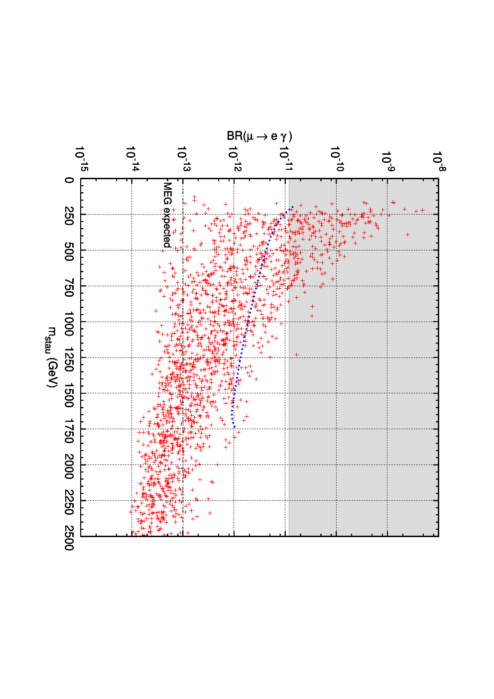
Let us now present the predictions of the model for other LFV processes. In Fig. 7, , and the conversion rate in the Titanium nucleus are plotted against for the same parameter choice as in Fig. 5. is not shown since, as discussed in Section 3.2, it is generally smaller than . Given the experimental upper limits shown in Table 2, is at present the most constraining LFV observable. Since , in agreement with Eq. (32) and with the correlation observed in type II seesaw models for large [9], is out of reach of super B factories, which are expected to achieve a sensivity of on its branching ratio [20]. conversion looks more promising, given that proposed experiments at Fermilab [42] and at J-PARK [43] aim at respective sensitivities of and on . If approved, these experiments would test the model well beyond the MEG reach.
In order to estimate the impact of non-universal (but flavour-blind) boundary conditions on the predictions for LFV observables, we performed a random scan of the soft scalar masses for different SO(10) multiplets between and , assuming a fixed value of the common gaugino mass parameter. The results for are shown in Fig. 7, where the blue dotted line77 7 In the universal case, radiative electroweak symmetry breaking does not take place for large values, which explains why the blue dotted line stops at . corresponds to the universal case . Relaxing the universality of soft scalar masses can enhance or suppress by up to 2 orders of magnitude, but most of the points still remain within the reach of MEG (unless the lightest slepton is very heavy).

As mentioned earlier, LFV observables provide much stronger constraints on the model studied in this paper than hadronic observables. A possible exception is represented by the indirect CP violation parameter in the kaon sector, . It is well known that is very sensitive to new sources of flavour and CP violation in the 1-2 down squark sector. In the present model, radiative corrections generate large off-diagonal entries both in the LL slepton mass matrix (which leads to large LFV rates) and in the RR down squark mass matrix. Moreover, order one phases in the PMNS matrix, hence in the couplings, are needed to account for the baryon asymmetry of the universe. Unfortunately, unknown extra SO(10) phases spoil the link between CP violation in the neutrino sector and the RG-induced CP violation in the sfermion mass matrices (see the discussion in Section 3.2). Nevertheless, barring cancellations between contributions carrying different phases, it is reasonable to expect a large imaginary part of . In Fig. 8, the contours of the supersymmetric contribution to are plotted in the plane for the same choice of parameters as in Fig. 5, assuming . While low values of would give too large a contribution to , a rather light superpartner spectrum can account for up to of its experimental value. According to Ref. [28], this is precisely what is needed in order to reconcile the SM prediction for with experiment.
6 Conclusions
We have studied flavour violation in a supersymmetric SO(10) implementation of the type II seesaw mechanism, which provides a predictive realization of triplet leptogenesis. In this scenario, the high-energy flavour parameters involved in the computation of the bayon asymmetry of the universe and of flavour-violating observables are determined in terms of the Standard Model fermion masses and mixing, up to mild model-dependent uncertainties. The overall size of the FCNC effects is then controlled by a few unknown flavour-blind parameters, while the ratios of FCNC rates for different flavour channels, such as , mainly depend on low-energy parameters.
The features of flavour violation in the SO(10) scenario studied in this paper present some interesting differences with the SU(5) implementation of the type II seesaw mechanism [9], because of additional contributions coming from the heavy matter fields crucial for leptogenesis. These give rise, for example, to radiative corrections to the soft mass matrices and controlled by the top quark Yukawa coupling. Moreover, the presence of a built-in leptogenesis mechanism provides a criterion for fixing the values of the unknown flavour-blind parameters, thus yielding testable predictions for the rates of flavour-violating processes. Imposing the conditions for successful leptogenesis together with the experimental constraints on FCNCs, we found that the predicted branching ratio for lies within the sensitivity of the MEG experiment if the superpartner spectrum is accessible at the LHC, while is out of reach of future super B factories. conversion on Titanium is also a promising process, with a predicted rate within the reach of proposed experiments at Fermilab and J-PARK even in regions of the parameter space where lies below the MEG sensitivity. Hadronic observables only receive small contributions once the experimental bounds on LFV processes are imposed, with the possible exception of .
We have also studied flavour-violating contributions to leptonic and hadronic EDMs, as well as to the parameter. The CKM and PMNS phases, together with new CP-violating phases associated with the SO(10) structure, can in principle induce sizable contributions to these observables, even if the soft terms are real at the high scale. The experimental bounds on LFV processes, however, prevent significant contributions to the EDMs, while a sizable contribution to (which might be necessary to account for its measured value) is still possible.
The predictivity of the scenario studied in this paper relies on the SO(10) relations between the flavour structures of the SM and heavy matter fields. These relations, however, only hold at the tree level and may be affected by model-dependent corrections from the non-renormalizable operators necessary to account for the measured quark and lepton masses. Nevertheless, the impact of these corrections on our results can be estimated to be mild.
The presence of heavy states below the GUT scale, besides inducing low-energy flavour and CP violation through radiative corrections, also has an impact on the superpartner spectrum. Indeed, their contribution to the beta functions leads to a relatively large value of the unified gauge coupling, which enhances the gauge contribution to the running of sfermion masses. One of the consequences of this is that the lightest neutralino turns out to be the LSP in an unusually large portion of the parameter space.
Finally, we have shown that the SO(10) implementation of the type II seesaw mechanism studied in this paper can be promoted to a consistent model including the dynamics of gauge symmetry breaking, doublet-triplet splitting consistent with the present experimental bounds on proton decay, and gauge coupling unification. The doublet-triplet splitting is achieved through a generalization of the missing vev mechanism. The proton decay rate is suppressed by arranging, without fine-tuning, a pair of Higgs doublets to lie at an intermediate scale. Gauge coupling unification is then restored by an appropriate splitting of the SU(5) components of the 54 containing the type II seesaw triplet, which in turn brings within from its experimental value, thus improving on the MSSM prediction. In passing, we provided an updated, comprehensive analysis of proton decay from D=5 and D=6 operators.
Acknowledgments
We thank F. Joaquim and A. Rossi for useful comments. The work of MF was supported in part by the Marie-Curie Intra-European Fellowship MEIF-CT-2007-039968. AR acknowledges partial support from the RTN European Program “UniverseNet” (MRTN-CT-2006-035863).
Appendix A SO(10) gauge symmetry breaking
The purpose of this appendix is to provide an explicit sector breaking the SO(10) gauge symmetry down to the SM gauge group. It is well known that this breaking can be realized by the most general renormalizable superpotential involving the following Higgs representations: one , one and one pair. In this case, both SM singlets in the acquire a nonzero vev. However, we need a multiplet with a vev aligned in the direction to implement the missing vev mechanism for doublet-triplet splitting (see Appendix B). In order to obtain such a vacuum alignment, we must introduce additional fields and consider a non-generic superpotential. A simple realization of this is provided by the following superpotential:
| (A.1) |
where is an SO(10) singlet and the contractions of SO(10) indices are understood. As shown below, the acquires a GUT-scale vev and therefore cannot be identified with the multiplet involved in the type II seesaw mechanism.
Altogether, eight SM singlets can acquire a nonzero vev at the GUT scale. We normalize their vevs as follows: , which breaks SO(10) down to its Pati-Salam subgroup, (), , and . In order to preserve supersymmetry, these vevs must satisfy F-flatness and D-flatness conditions. The solution to these constraints reads88 8 Let us mention for completeness that the D-flatness and F-flatness conditions admit another solution characterized by and all other vevs nonzero. This solution would also be satisfactory for our purposes, but we stick to the first one for definiteness.:
| (A.2) |
together with . If the dimensionless couplings are of order one, then all nonzero vevs are of order , the unique mass parameter in . Therefore SO(10) is broken down to the SM gauge group in one step. The two vevs are aligned along the and directions, respectively; in the rest of the paper we will rename them and .
The SM vacuum defined by Eq. (A.2) provides all uneaten chiral superfields with a GUT-scale mass, except for a pair of charged states with quantum numbers , which remains massless99 9 In the alternative vacuum characterized by , the massless states are .. This problem can be cured by adding the following terms to :
| (A.3) |
This does not modify the vacuum alignment discussed above and does not introduce extra mass parameters either. The F-flatness conditions imply that the does not acquires a vev. The coupling is sufficient to make the unwanted massless states heavy, while the coupling guarantees that all components are also massive.
For completeness, we give the masses of the and gauge bosons, which can mediate proton decay through operators (see Appendix B.3):
| (A.4) |
where is the SO(10) gauge coupling.
We remark that the desired vev alignment is obtained because several couplings allowed by the SO(10) gauge symmetry are absent in Eq. (A.1). In fact, one can add mass terms for and without upsetting the vev alignment. On the contrary, it is crucial to forbid all couplings except and . We do not try to justify the non-generic form of by global symmetries, which would require a more complicated set of fields and interactions.
Note finally that it is possible to align the vev of one of the two ’s without introducing the SO(10) singlet . In fact, if one replaces in Eq. (A.1) by a bare mass , the F-flatness equations still have a solution with and a second one with , all other vevs being nonzero. This is sufficient to realize the doublet-triplet splitting, but this requires the presence of two mass parameters ( and ) in .
Appendix B Doublet-triplet splitting and proton decay
In this appendix, we provide an explicit doublet-triplet splitting mechanism for the SO(10) scenario studied in this paper, and derive the conditions imposed by the non-observation of proton decay on the heavy spectrum.
B.1 Doublet-triplet splitting
In the SO(10) implementation of the type II seesaw mechanism considered in this paper, up quark masses arise from the superpotential couplings , while down quark and charged lepton masses arise from the couplings . The MSSM Higgs doublet should therefore reside mainly in the in order to account for the large top quark mass, while the Higgs doublet should contain a significant component, and we require that it also has a non-vanishing component1010 10 Indeed, the leptogenesis scenario of Ref. [7] assumes that the dominant decay modes of the heavy matter fields preserve , which is guaranteed if contains a non-negligible component.. The doublet-triplet splitting mechanism, besides rendering all colour triplets coupling to light matter fields heavy, should therefore leave and an admixture of and massless.
This can be achieved by a generalization of the missing vev mechanism [29] involving an additional Higgs multiplet and an adjoint Higgs field with a non-vanishing vev in the direction (which motivates the choice made for in Appendix A). The superpotential that accomplishes the desired doublet-triplet splitting reads:
| (B.1) |
where the third term also plays a role in SO(10) symmetry breaking (and therefore appears in Eq. (A.1)), while the coupling is optional. As in the case of Eq. (A.1), this is not the most general superpotential for the fields involved. After SO(10) symmetry breaking, one obtains the following doublet and triplet mass matrices, written in the (left) and (right) bases:
| (B.2) |
From Eq. (B.2) we can see that all colour triplets and two pairs of Higgs doublets acquire GUT-scale masses, while and a combination of and remain massless:
| (B.3) |
where the Higgs mixing angle is given by (with no loss of generality, we assume and to be real):
| (B.4) |
Note that the alignment of the vev along the direction is crucial for the splitting of the doublet and triplet components.
A few comments are in order about the above doublet-triplet mechanism. First, the SO(10)-breaking sector contains a representation with a vev in the Pati-Salam direction, whose couplings to and must be forbidden as they would make all Higgs doublets heavy. On the contrary, the coupling involved in the seesaw mechanism is harmless since does not acquire a vev. Second, the mass term in Eqs. (A.1) and (B.1) is crucial both for GUT symmetry breaking and for the doublet-triplet splitting: if it were absent, F-flatness would imply either , leaving the SO(10) rank unbroken, or , leaving a pair of colour triplets massless.
B.2 Higgs-mediated proton decay
In general, giving GUT-scale masses to the colour Higgs triplets is not enough to suppress the proton decay rate below its experimental upper limit. To achieve this, one must impose additional constraints on the triplet mass matrix. We show below that this can be done in a simple way in the doublet-triplet splitting scenario presented above.
Let us first adapt the standard computation of the Higgs-mediated proton decay rate [44, 45, 46, 47] to our case. Upon integrating out the heavy Higgs triplet superfields, one obtains the following D=5 operators:
| (B.5) |
where the contraction of gauge indices is understood, and the dimensionful coefficients and generated by the superpotential (1) are given by1111 11 Note that the flavour structure of and is the same as in the minimal SU(5) model. This is an obvious consequence of the way the SM matter fields are embedded into SO(10) representations.:
| (B.6) |
where is the entry of the inverse triplet mass matrix. Since colour invariance implies and , the dominant proton decay modes arising from the above operators involve a kaon, and in practice dominates. The corresponding amplitude is obtained by “dressing” the D=5 operators of Eq. (B.5) with gaugino/higgsino loops. If the first two generation squarks are close in mass, as the observed weakness of hadronic flavour-violating processes may suggest, the dominant contributions come from the wino dressing of the operator and from the charged higgsino dressing of the operator. Here we consider only the former contribution; the latter (which is significant for the channel only) would give a stronger constraint on only for large values of . The proton partial decay width then reads:
| (B.7) |
where MeV is the pion decay constant; is the hadronic parameter defined by , where is the proton spinor and the parenthesis indicates the contraction of Lorentz indices; D and F are chiral Lagrangian parameters; and is the Wilson coefficient of the four-fermion operator . The most recent lattice determination of is [48], while an analysis of hyperon decay measurements gives and [49]. The Wilson coefficients read:
| (B.8) |
where is a renormalization factor, is the CKM matrix, the coefficients are expressed in the basis , and the loop function is given by ( is the wino mass):
| (B.9) |
For degenerate sfermion masses () and a hierarchy , reduces to to a good approximation. In Eq. (B.8), the quantity is evaluated at the GUT scale, where the operator is generated. The renormalization factor contains a short-distance piece which accounts for the renormalization of the superpotential operator from to the supersymmetry breaking scale (here identified with ), and a long-distance piece which encodes the renormalization of the four-fermion operator from to GeV. The latter is given by:
| (B.10) |
and the former by (neglecting the Yukawa contributions):
| (B.11) |
where runs over all mass thresholds between and , and are the beta function coefficients between and . Given the hierarchy among the quark Yukawa couplings at the GUT scale, one has , with:
| (B.12) |
where and (, ) are high-energy phases, and the sum is dominated by the term (i.e. by the loops).
We are now in a position to derive a lower bound on from the experimental constraint yrs ( C.L.) [50]. For definiteness, we consider the model (ii) of Section 4.3 with GeV, and a spectrum close to the one of Fig. 6, with squark masses in the TeV range (except for the lightest stop), slepton masses around GeV and GeV. This spectrum gives . Evaluating the Yukawa couplings at the GUT scale, we find , , , and . Depending on the values of the high-energy phases, a partial cancellation between the and the contributions is possible. Here we do not consider this possibility and keep only the dominant contribution, which gives:
| (B.13) |
where we have replaced by an average value , and (to be compared with in the MSSM with ) takes into account the various thresholds shown in Fig. 1. From Eqs. (B.7) and (B.13), we finally obtain:
| (B.14) |
which yields the upper bound , where we have restored the approximate dependence of the proton decay amplitude (one can indeed see from Eq. (B.12) that and scale as ). This bound is a conservative one, and several effects could relax it: there are still large uncertainties on the hadronic parameter ; overestimates the running of the coefficients, since it does not include the Yukawa contribution; a superpartner spectrum characterized by heavier sfermions and/or a stronger sfermion/gaugino mass hierarchy would reduce the proton decay amplitude; corrections to the mass relation could affect the couplings of the Higgs triplets to quarks and leptons; and finally, some sfermion mixing patterns compatible with the observed level of flavour violation can significantly reduce the proton decay amplitude [51].
Let us now translate this bound into constraints on the doublet-triplet splitting parameters. From Eq. (B.2) we have:
| (B.15) |
where we made use of and . Since the SO(10) gauge symmetry is broken in one step (see Appendix A), and the desired suppression of with respect to its natural value can be achieved by a partial cancellation in the combination , or by taking and in the GeV range, where the lower value corresponds to the conservative bound on . Note that would not help, since the upper bound on becomes stricter for smaller values of . In this paper we take1212 12 Note that the mass scale GeV can be generated by an interaction term with , where is the SO(10) singlet introduced in Appendix A. GeV in order to avoid a strong cancellation among unrelated superpotential parameters. One can check that all colour Higgs triplets acquire GUT-scale masses in this case, while one pair of Higgs doublet sits at the intermediate scale . The consequences for gauge coupling unification are discussed in Appendix C, and summarized in Section 4.3.
B.3 Gauge-mediated proton decay
Let us now discuss the contribution of SO(10) gauge interactions to proton decay [47]. Due to the way the SM matter fields are embedded into SO(10) representations, there are no new gauge contributions with respect to the SU(5) case, i.e. only the and gauge bosons mediate proton decay. The dominant decay mode from exchange is , and its rate is given by (neglecting the non-gauge contributions, which are subdominant):
| (B.16) |
where is the hadronic parameter defined by , D and F are the same chiral Lagrangian parameters as above, and and are the Wilson coefficients of the four-fermion operators and , respectively. The most recent lattice determination of is [48]. The Wilson coefficients take the same form as in minimal SU(5):
| (B.17) |
where is the mass of the heavy gauge bosons. The long-distance piece of the renormalization factor is given by Eq. (B.10), while its short-distance piece reads:
| (B.18) |
where, as in Eq. (B.11), the Yukawa contributions have been neglected, and runs over all mass thresholds between and . Together with Eq. (B.17), Eq. (B.16) gives:
| (B.19) |
to be compared with the experimental upper bound yrs ( C.L.) [52]. In Eq. (B.19), and are the reference MSSM values. Consider now the model (i) of Section 4.3 with GeV, GeV, GeV and the same heavy fermion spectrum as in Fig. 1. At the one-loop level and omitting both low-energy and GUT thresholds, one obtains , GeV and . These values are at odds with the experimental limit on the proton lifetime (assuming leads to yrs). On the contrary, for model (ii) with the spectrum of Fig. 1 (with GeV, GeV and GeV), one finds , GeV and , leading to yrs for . We shall therefore adopt model (ii) as our reference model, although model (i) may be viable if 2-loop running and threshold effects conspire to increase the GUT scale. Also, the corrections needed to depart from the minimal SU(5) relation will in general modify Eq. (B.17) by introducing non-trivial fermion mixing angles in the heavy gauge boson couplings, and this could significantly reduce the proton decay rate [53].
B.4 Proton decay from non-renormalizable operators
For completeness, we mention that proton decay could also be induced by non-renormalizable superpotential operators of the form:
| (B.20) |
where is the cutoff, and the SU(5)-singlet component of the acquires a GUT-scale vev. These operators, if present, will generate the operators of Eq. (B.5) after SO(10) symmetry breaking. In order to avoid a confict with the experimental bound on proton lifetime, they must either be forbidden by some symmetry, or the ones involving light generation fields must be suppressed by small coefficients . This is actually what one would expect in a theory of flavour capable of explaining the hierarchy of fermion masses. Note that the required suppression of the coefficients is less severe than in conventional SO(10) models, where the dangerous operators, of the form , have dimension 5.
Appendix C Intermediate scales and gauge coupling unification
In this appendix, we study the constraints imposed by the requirement of successful gauge coupling unification on the extra heavy states present below the GUT scale, using 1-loop renormalization group equations.
As shown in Appendix B.2, the experimental constraint on the rate can easily be satisfied by allowing a pair of Higgs doublets to lie at an intermediate scale. This tends to spoil unification, but we will show that the problem can be cured by splitting the components of the . In fact, it is also desirable to give GUT-scale masses to some components of the SU(5) multiplets and contained in the in order to preserve perturbative unification. Indeed, the presence of additional chiral superfields at intermediate scales increases the value of the unified gauge coupling with respect to the MSSM. One has to check that a Landau pole is not reached soon above (or even below) the GUT scale, because this would make the predictions of the model very sensitive to the effects of higher-dimensional operators. In the SO(10) scenario studied in this paper, keeping the full close to the seesaw scale would give , and the Landau pole would be reached at a scale . Thus, motivated both by perturbativity and by proton decay, we are led to split the and multiplets, keeping below the GUT scale only the components that are necessary for the seesaw mechanism and for leptogenesis, together with possible additional components needed to achieve unification.
As is customary, we define as the scale where and meet. Denoting by the masses of the intermediate-scale states and by () their contributions to the beta-function coefficients, the 1-loop predictions for , and read:
| (C.1) | ||||
| (C.2) | ||||
| (C.3) |
where the superscript “” refers to MSSM quantities, with , GeV, , and
| (C.4) |
Given the fact that the MSSM prediction for significantly deviates from the measured value (using 2-loop RGEs and including low-energy supersymmetric thresholds, one finds , which corresponds to a deviation), a positive contribution of the extra states to Eq. (C.1) would be welcome.
Replacing Eq. (C.2) into Eq. (C.3) one finds:
| (C.5) |
The third term always increases , while the second one can decrease or increase it, depending on whether is smaller or larger than . However, the contribution of the second term is bounded by the requirement GeV coming from proton decay (see Apprendix B.3). Therefore, in order to avoid a too large value of , the additional intermediate-scale fields besides the ones needed to realize leptogenesis and to suppress proton decay [namely , and/or , and ] should better be SU(2)L singlets. There are two such components: and . Since is an electroweak singlet, it does not affect nor (but it corrects the prediction for ). Adding only would push above the Planck scale. We are thus left with two possibilities: (i) intermediate ; (ii) intermediate and . The right-hand side of Eq. (C.1) reads, for each of the two cases:
| (C.6a) | ||||
| (C.6b) |
while and are given by the same expression in both cases:
| (C.7) | ||||
| (C.8) |
where we assumed . From the above equations, we can see that lowering decreases as desired (and improves the prediction for ), but decreases .
Let us first consider case (i). Assuming GeV, GeV and GeV (as well as , , and to fix the masses of the heavy pairs), we obtain, at the 1-loop level:
| (C.9) |
In this case, the prediction for is only slightly larger than in the MSSM, and the value of the unified coupling remains reasonable. Unfortunately, the unification scale lies almost one order of magnitude below the MSSM prediction, which leads to a too fast proton decay rate (see Appendix B.3). Gauge coupling unification is approximately preserved if and are varied while keeping the ratio fixed. In particular, increasing while keeping slightly increases (and decreases and ). For instance, for GeV, one obtains , GeV and . Still the unification scale is dangerously close to the proton decay bound.
Let us now consider case (ii). As anticipated, only is affected by the presence of below . This gives the possibility of increasing with respect to case (i) by increasing , while correcting the prediction for by adjusting . For instance, the choice GeV, GeV and GeV gives, at the 1-loop level:
| (C.10) |
In this case, unification works better than in the MSSM. Indeed, we checked that the prediction for , including low-energy thresholds and the 2-loop MSSM running, matches the measured value within . Moreover, there is no conflict between the value of and proton decay, and the Landau pole lies one order of magnitude above . From Eq. (Cb), we can see that the contributions of and cancel if . Therefore, unification is still preserved if the masses of the various states are varied while keeping and GeV.
| Operator | Massive components | Mass |
|---|---|---|
The splitting of the masses of the components needed to realize case (ii) can be achieved with the set of operators shown in Table 3, where is the Pati-Salam invariant vev of the , is the vev of the , which is aligned along the direction, and has no vev (see Appendix A). At the renormalizable level, only and acquire a (GUT-scale) mass. The dimension-5 operators provide as well as (more precisely, when the GUT-scale masses of the and components are taken into account, and are further suppressed by a mild seesaw-like mechanism). Finally, the dimension-6 operator generates .
Appendix D Renormalization group equations
Below , the superpotential terms (2) and (3) read, in terms of the SM components (2):
| (D.1) |
where Clebsch-Gordan coefficients have been factorized out, and contractions of and indices are understood. The interactions of fields with GUT-scale masses, namely the right-handed neutrinos and the components of and other than the light Higgs doublets, have been omitted1313 13 Similarly, the interactions of the components with GUT-scale masses should not appear in Eq. (D.1), nor in the RGEs.. The boundary conditions at the GUT scale for the superpotential couplings and mass parameters are:
| (D.2) | ||||
where the Higgs mixing angle is defined by Eq. (B.3), and is the vev of the singlet component of the . We did not write boundary conditions for the masses of the components, since, as discussed in Appendix C, they are assumed to be split by operators not included in the superpotential (3).
The soft supersymmetry breaking terms for the SO(10) fields are defined by:
| (D.3) |
where we used the same notation for the chiral multiplets and for their scalar components, are the SO(10) gauginos, and we omitted the -terms. The soft terms of the SM components are given, at the GUT scale, by the following boundary conditions:
| (D.4) | ||||
The boundary conditions for the -terms, not included in the above list, are analogous to the ones for the corresponding Yukawa couplings. One has for instance:
| (D.5) |
In the numerical study of Section 5, we solved the 1-loop RGEs for all superpotential couplings and soft terms below . For brevity, we only list below the RGEs for the MSSM parameters, which are sufficient for a leading-log analysis of flavour-violating effects. Let us first recall the 1-loop RGEs for gauge couplings and gaugino masses:
| (D.6) |
| (D.7) |
where , being the renormalization scale and a reference scale, is the second Casimir invariant of the group , is the Dynkin index of the representation , and the sum in runs over all chiral superfields with mass smaller than .
The 1-loop RGEs for the MSSM Yukawa couplings are:
| (D.8) |
| (D.9) |
| (D.10) |
The 1-loop RGEs for the MSSM soft sfermion masses are:
| (D.11) |
| (D.12) |
| (D.13) |
| (D.14) |
| (D.15) |
where the hypercharge D-term contribution is given by:
| (D.16) |
The mixing terms appearing in the RGEs for and , although absent at , are generated by the RGE evolution and must be included for consistency.
Finally, the 1-loop RGEs for the MSSM -terms are:
| (D.17) |
| (D.18) |
| (D.19) |
References
- [1] S. Weinberg, Phys. Rev. Lett. 43 (1979) 1566.
- [2] P. Minkowski, Phys. Lett. B 67 (1977) 421; M. Gell-Mann, P. Ramond and R. Slansky, in Supergravity, P. van Nieuwenhuizen and D.Z. Freedman (eds.), North Holland Publ. Co., 1979, p. 315; T. Yanagida, in Proc. of the Workshop on the Baryon Number of the Universe and Unified Theories, O. Sawada and A. Sugamoto (eds.), Tsukuba, Japan, 13-14 Feb. 1979, p. 95; S. L. Glashow, in Quarks and Leptons, Cargèse Lectures, 9-29 July 1979, Plenum, New York, 1980, p. 687; R. N. Mohapatra and G. Senjanovic, Phys. Rev. Lett. 44 (1980) 912.
- [3] M. Fukugita and T. Yanagida, Phys. Lett. B 174 (1986) 45.
- [4] F. Borzumati and A. Masiero, Phys. Rev. Lett. 57 (1986) 961.
- [5] M. Magg and C. Wetterich, Phys. Lett. B 94 (1980) 61; G. Lazarides, Q. Shafi and C. Wetterich, Nucl. Phys. B 181 (1981) 287; R. N. Mohapatra and G. Senjanovic, Phys. Rev. D 23 (1981) 165. See also J. Schechter and J. W. F. Valle, Phys. Rev. D 22 (1980) 2227.
- [6] H. Georgi, AIP Conf. Proc. 23 (1975) 575; H. Fritzsch and P. Minkowski, Annals Phys. 93 (1975) 193.
- [7] M. Frigerio, P. Hosteins, S. Lavignac and A. Romanino, Nucl. Phys. B 806 (2009) 84 [arXiv:0804.0801 [hep-ph]].
- [8] P. J. O’Donnell and U. Sarkar, Phys. Rev. D 49 (1994) 2118 [arXiv:hep-ph/9307279]; E. Ma and U. Sarkar, Phys. Rev. Lett. 80 (1998) 5716 [arXiv:hep-ph/9802445]; T. Hambye and G. Senjanovic, Phys. Lett. B 582 (2004) 73 [arXiv:hep-ph/0307237].
- [9] A. Rossi, Phys. Rev. D 66 (2002) 075003 [arXiv:hep-ph/0207006].
- [10] J. Hisano, H. Murayama and T. Yanagida, Phys. Rev. D 49 (1994) 4966; Z. Berezhiani and Z. Tavartkiladze, Phys. Lett. B 409 (1997) 220 [arXiv:hep-ph/9612232]; Y. Nomura and T. Yanagida, Phys. Rev. D 59 (1999) 017303 [arXiv:hep-ph/9807325]; J. L. Rosner, Phys. Rev. D 61 (2000) 097303; Z. Berezhiani and A. Rossi, Nucl. Phys. B 594 (2001) 113 [arXiv:hep-ph/0003084]; T. Asaka, Phys. Lett. B 562 (2003) 291 [arXiv:hep-ph/0304124]; K. S. Babu, I. Gogoladze, P. Nath and R. M. Syed, Phys. Rev. D 74 (2006) 075004 [arXiv:hep-ph/0607244]; S. M. Barr, Phys. Rev. D 76 (2007) 105024 [arXiv:0706.1490 [hep-ph]]; M. Malinsky, Phys. Rev. D 77 (2008) 055016.
- [11] J. A. Casas and A. Ibarra, Nucl. Phys. B 618 (2001) 171 [arXiv:hep-ph/0103065].
- [12] F. R. Joaquim and A. Rossi, Phys. Rev. Lett. 97 (2006) 181801 [arXiv:hep-ph/0604083], Nucl. Phys. B 765 (2007) 71 [arXiv:hep-ph/0607298].
- [13] R. Barbieri and L. J. Hall, Phys. Lett. B 338 (1994) 212 [arXiv:hep-ph/9408406]; R. Barbieri, L. J. Hall and A. Strumia, Nucl. Phys. B 445 (1995) 219 [arXiv:hep-ph/9501334].
- [14] L. J. Hall, V. A. Kostelecky and S. Raby, Nucl. Phys. B 267 (1986) 415.
- [15] T. Schwetz, M. A. Tortola and J. W. F. Valle, New J. Phys. 10 (2008) 113011 [arXiv:0808.2016 [hep-ph]].
- [16] I. Masina and C. A. Savoy, Nucl. Phys. B 661, 365 (2003) [arXiv:hep-ph/0211283].
- [17] P. Paradisi, JHEP 0510, 006 (2005) [arXiv:hep-ph/0505046].
- [18] M. Ciuchini, A. Masiero, P. Paradisi, L. Silvestrini, S. K. Vempati and O. Vives, Nucl. Phys. B 783, 112 (2007) [arXiv:hep-ph/0702144].
- [19] F. Gabbiani, E. Gabrielli, A. Masiero and L. Silvestrini, Nucl. Phys. B 477 (1996) 321 [arXiv:hep-ph/9604387].
- [20] M. Bona et al., arXiv:0709.0451 [hep-ex].
- [21] P. Brax and C. A. Savoy, Nucl. Phys. B 447 (1995) 227 [arXiv:hep-ph/9503306].
- [22] I. Masina, Nucl. Phys. B 671 (2003) 432 [arXiv:hep-ph/0304299]; Y. Farzan and M. E. Peskin, Phys. Rev. D 70 (2004) 095001 [arXiv:hep-ph/0405214].
- [23] J. Hisano, M. Nagai and P. Paradisi, arXiv:0812.4283 [hep-ph].
- [24] M. Pospelov and A. Ritz, Annals Phys. 318 (2005) 119 [arXiv:hep-ph/0504231].
- [25] B. C. Regan, E. D. Commins, C. J. Schmidt and D. DeMille, Phys. Rev. Lett. 88 (2002) 071805.
- [26] G. W. Bennett et al. [Muon (g-2) Collaboration], arXiv:0811.1207 [hep-ex].
- [27] C. A. Baker et al., Phys. Rev. Lett. 97 (2006) 131801 [arXiv:hep-ex/0602020].
- [28] A. J. Buras and D. Guadagnoli, Phys. Rev. D 78 (2008) 033005 [arXiv:0805.3887 [hep-ph]]; A. J. Buras and D. Guadagnoli, arXiv:0901.2056 [hep-ph].
- [29] S. Dimopoulos and F. Wilczek, preprint NSF-ITP-82-07, August 1981 (unpublished) and Supersymmetric Unified Models, in Proceedings of the Erice Summer School (A. Zichichi ed.), 1981, pp. 237-249; M. Srednicki, Nucl. Phys. B 202 (1982) 327; K. S. Babu and S. M. Barr, Phys. Rev. D 48 (1993) 5354 [arXiv:hep-ph/9306242].
- [30] M. L. Brooks et al. [MEGA Collaboration], Phys. Rev. Lett. 83 (1999) 1521 [arXiv:hep-ex/9905013].
- [31] U. Bellgardt et al. [SINDRUM Collaboration], Nucl. Phys. B 299 (1988) 1.
- [32] C. Dohmen et al. [SINDRUM II Collaboration.], Phys. Lett. B 317, 631 (1993); J. Kaulard et al. [SINDRUM II Collaboration], Phys. Lett. B 422, 334 (1998).
- [33] B. Aubert [The BABAR Collaboration], arXiv:0908.2381 [hep-ex].
- [34] C. Amsler et al. [Particle Data Group], Phys. Lett. B 667 (2008) 1.
- [35] E. Barberio et al. [Heavy Flavor Averaging Group (HFAG) Collaboration], arXiv:0704.3575 [hep-ex].
- [36] T. Aaltonen et al. [CDF Collaboration], Phys. Rev. Lett. 100 (2008) 101802 [arXiv:0712.1708 [hep-ex]].
- [37] J. Hisano, T. Moroi, K. Tobe and M. Yamaguchi, Phys. Rev. D 53, 2442 (1996) [arXiv:hep-ph/9510309].
- [38] G. Isidori and A. Retico, JHEP 0209 (2002) 063 [arXiv:hep-ph/0208159]; G. Isidori and P. Paradisi, Phys. Lett. B 639 (2006) 499 [arXiv:hep-ph/0605012].
- [39] G. Degrassi, P. Gambino and P. Slavich, Comput. Phys. Commun. 179, 759 (2008) [arXiv:0712.3265 [hep-ph]].
- [40] M. Ciuchini et al., JHEP 9810 (1998) 008 [arXiv:hep-ph/9808328].
- [41] L. M. Barkov et al., PSI Proposal R-99-05 (1999); S. Ritt [MEG Collaboration], Nucl. Phys. Proc. Suppl. 162, 279 (2006); J. Adam et al. [MEG collaboration], arXiv:0908.2594 [hep-ex].
- [42] R. M. Carey et al. [Mu2e Collaboration], “Proposal to search for with a single event sensitivity below ”.
- [43] The PRIME working group, “Search for the Conversion Process at an Ultimate Sensitivity of the Order of with PRISM”, unpublished; LOI to J-PARC 50-GeV PS, LOI-25, http://psux1.kek.jp/jhf-np/LOIlist/LOIlist.html
- [44] J. R. Ellis, D. V. Nanopoulos and S. Rudaz, Nucl. Phys. B 202 (1982) 43.
- [45] P. Nath, A. H. Chamseddine and R. L. Arnowitt, Phys. Rev. D 32 (1985) 2348.
- [46] J. Hisano, H. Murayama and T. Yanagida, Nucl. Phys. B 402 (1993) 46 [arXiv:hep-ph/9207279].
- [47] For a recent review on proton decay, see P. Nath and P. Fileviez Perez, Phys. Rept. 441 (2007) 191 [arXiv:hep-ph/0601023].
- [48] Y. Aoki et al. [RBC-UKQCD Collaboration], Phys. Rev. D 78 (2008) 054505 [arXiv:0806.1031 [hep-lat]].
- [49] N. Cabibbo, E. C. Swallow and R. Winston, Ann. Rev. Nucl. Part. Sci. 53 (2003) 39 [arXiv:hep-ph/0307298].
- [50] K. Kobayashi et al. [Super-Kamiokande Collaboration], Phys. Rev. D 72 (2005) 052007 [arXiv:hep-ex/0502026].
- [51] B. Bajc, P. Fileviez Perez and G. Senjanovic, Phys. Rev. D 66 (2002) 075005 [arXiv:hep-ph/0204311].
- [52] H. Nishino et al. [Super-Kamiokande Collaboration], Phys. Rev. Lett. 102 (2009) 141801 [arXiv:0903.0676 [hep-ex]].
- [53] I. Dorsner and P. Fileviez Perez, Phys. Lett. B 625 (2005) 88 [arXiv:hep-ph/0410198].