Supersymmetric particle mass measurement with the boost-corrected contransverse mass
Abstract:
A modification to the contransverse mass () technique for measuring the masses of pair-produced semi-invisibly decaying heavy particles is proposed in which is corrected for non-zero boosts of the centre-of-momentum (CoM) frame of the heavy states in the laboratory transverse plane. Lack of knowledge of the mass of the CoM frame prevents exact correction for this boost, however it is shown that a conservative correction can nevertheless be derived which always generates an value which is less than or equal to the true value of in the CoM frame. The new technique is demonstrated with case studies of mass measurement with fully leptonic events and with SUSY events possessing a similar final state.
Keywords:
SUSY, fit, contransverse1 Introduction
Techniques for measuring the masses of pair-produced particles decaying semi-invisibly through short decay chains at hadron colliders have attracted considerable interest. The principle motivation for the development of such techniques is the measurement of the masses of supersymmetric particles (‘sparticles’) at the Large Hadron Collider [1, 2, 3, 4, 5, 6, 7, 8, 9, 10, 11, 12, 13, 14, 15, 16], however they may be applied more widely to measure the mass of the top quark at the Tevatron [17] or LHC [18], or to identify fully leptonic events [19].
Recently [9] a straightforward new variable, the ‘contransverse mass’ (), was proposed which enables the measurement of a simple analytical combination of the masses of the pair-produced heavy states () and their invisible decay products . The contransverse mass is defined by
| (1) | |||||
| (2) |
where are the visible products of each decay chain, is the tranverse momentum vector of and
| (3) |
It can be shown [9] that is in general bounded from above by a quantity dependent upon the masses and . If then the distribution of event values possesses an end-point at:
| (4) |
Consequently a measurement of the gradient and intercept of the linear function describing the dependence of on allows both and to be measured independently.
Despite the simplicity and ease-of-use of the contransverse mass technique, it suffers from two principle draw-backs [9]. The first is that is not invariant under Lorentz boosts of the centre-of-momentum (CoM) frame in the laboratory transverse plane. Consequently if the system recoils in the transverse plane against upstream object(s) such as ISR jets then the value of calculated in the laboratory frame is not in general equal to that calculated in the CoM frame. values can be generated which are greater than and as a result the end-point can be smeared (see e.g. Figure 2 in Ref. [9]). The second draw-back is apparent when attempting to measure and independently in events with non-zero visible masses using Eqn. (4). The requirement can significantly reduce the available event statistics and require the accumulation of very large integrated luminosity, even for channels with relatively large . This problem is illustrated clearly in Figure 3 in Ref. [9]. This paper will seek to address these two problems and demonstrate the utility of the technique through two case-studies. In the process we shall identify a further problem with using Eqn. (4) to measure masses independently, but develop an alternative strategy for two-step sequential two-body decay chains combining end-point measurements with conventional invariant mass end-point constraints. We shall also investigate the use of the transverse boost dependence of to measure masses independently, but find that this technique suffers from similar problems.
The structure of the paper is as follows. Section 2 will study the transformation properties of under contra-linear and co-linear Lorentz boosts of , leading to the development of a procedure for correcting for co-linear boosts. Section 3 will discuss the shape of the resulting distributions. Section 4 will propose a new method for maximising the available event statistics when measuring and independently with Eqn. (4) by removing the requirement. This section will also develop a technique through which and can in principle be measured independently by using the transverse boost dependence of . Section 5 will investigate these techniques with LHC case studies measuring the masses of the top quark, and neutrino with fully-leptonic events, and the masses of SUSY particles decaying to a similar final state. Section 6 will conclude.
2 Transformation properties of
2.1 Equal magnitude contra-linear boosts
It is instructive to consider first the transformation properties of under contra-linear equal magnitude boosts, in which and move in opposite directions with equal momentum. is derived from the quantity given by
| (5) | |||||
| (6) |
and this was shown in Ref. [9] to be invariant under such boosts. By contrast is not in general invariant under such boosts, however the position of the end-point, , is. The reason for this can be understood by observing that one can rewrite Eqn. (5) in the following form in the CoM frame:
| (7) |
Comparing with Eqn. (1) and noting that this shows that , with equality when . Now , like , is bounded from above by and so one finds finally that . It is interesting to note additionally that equals when and are co-linear in the rest frames and hence the necessary and sufficient criteria for are that and in the rest frames while in the CoM frame.
A similar argument applies when the transverse mass undergoes co-linear equal magnitude boosts, and the result is similar, namely that is not invariant under arbitrary transverse boosts but nevertheless possesses a boost-invariant end-point. It is interesting to note that in this case the necessary and sufficient conditions for are in some sense the complement of those in the case: here and in the rest frame(s) of the parent particle(s) while in the event CoM frame. Of course if and are the sole products of the decay of the same parent then the first and second criteria are generally satisfied through conservation of momentum.
2.2 Equal magnitude co-linear boosts
The contransverse mass is invariant by construction under co-linear equal magnitude boosts of and in the beam () direction, by virtue of its dependence purely on transverse quantities. Consequently is similarly invariant. In the presence of co-linear equal magnitude boosts in the CoM transverse plane however, equivalent to a single global transverse boost, the values of both and can depend on the magnitude and direction of the boost. For instance, when Eqn. (4) becomes:
| (8) |
where , is the net transverse momentum of upstream objects (ISR jets etc.) generating the boost,
| (9) |
and .
With sufficient statistics one might hope to use Eqn. (8) to measure and separately by measuring as a function of . This possibility is considered further in Section 4. With limited statistics however it would be useful to be able to transform such that its value always lies below the end-point given by Eqn. (4). In this case one sacrifices the ability to measure and independently using the dependence of in order to maximise statistics near the end-point, while limiting smearing beyond the end-point due to integration over .
The approach we shall take will involve boosting the four-momenta of the visible decay products back into the CoM frame with boost factor , prior to calculating . If we know neither the sign nor the magnitude of then the minimum value of that we can obtain by varying the assumed value of is the one-dimensional analogue of given by defined by
| (10) | |||||
| (11) |
where and we have assumed that the boost lies in the direction. is invariant under arbitrary boosts in the plane for the same reason that is invariant under boosts in the direction. It represents a conservative lower bound on the value of measured in the CoM frame. The criterion for to equal in any given frame, and hence for to be minimised in that frame, is that , where is defined by
| (12) |
As an aside, it is interesting to consider at this point the possibility of using defined by Eqn. (5), rather than , and attempting to perform a correction for longitudinal boosts along the beam direction. In this case we know neither the sign nor the magnitude of the -boost and so by the above argument the appropriate quantity to use is the two-dimensional analogue of , which is just as we have been using already. The criterion for to equal is by analogy with Eqn. (12)
| (13) |
which is equivalent to setting as required by Eqn. (7).
Now in fact we do know the sign of the required boost, because we know the direction in the transverse plane of the upstream momentum. Defining this direction to be the direction we need to boost and in this same direction (i.e. use ) to correct for the original boost of the CoM frame, which must have been in the direction. Such a boost monotonically increases and hence monotonically increases the transformed value of towards as . Let us define now and to be the values of and measured in the lab frame and and to be the equivalent values obtained after boosting and . If then increases monotonically from towards as (see Figures 1 and 2). Consequently in this case the least conservative lower bound on we can obtain is . If on the other hand is negative then as and increase first decreases from towards its minimum value of (at ) before increasing again towards (see Figures 1 and 2). In this case, without further information, the best we can do is set .


Fortunately however we have not yet exhausted the possibilities for boost correction. Observe first that when boosting and the boost factor is given by where is the assumed value of the energy of the CoM frame in the lab frame. Consequently increasing the value of is equivalent to decreasing , and vice versa. Hence if increases (decreases) monotonically with increasing and we set to a value less than (greater than) , the value of we obtain provides a conservative lower bound on . Now if then always increases with increasing (see Figure 1) and hence it decreases with increasing (see Figure 3 – upper curve). In this case we should set to the upper bound on , boost and , and obtain a conservative lower bound on from the value of in this frame. If the situation is more complicated (see Figure 3 – lower curve). In this case, if after boosting with set to both the upper and lower bounds on then the least conservative lower bound on is given by the value of with set to the lower bound on . Conversely if in both these cases then the least conservative lower bound on is given by the value of with set to the upper bound on . If with set to the lower bound on but with set to the upper bound on then could be as low as and so this should be used as the least conservative lower bound on .

In fact we can indeed obtain both upper and lower bounds on . An upper bound is provided by the proton-proton centre of mass energy while the total visible energy of the decay products provides a lower bound. This latter quantity is calculated by summing the energies of the visible decay products with the net transverse momentum of the invisible decay products11 1 If a lower bound on the masses of the individual invisible decay products can be assumed then conservatively one can use in instead of to obtain an improved bound on . given by . equals the total energy of the invisible decay products only when these are massless, co-linear, and moving in the transverse plane, and so in general . Below we shall denote values of obtained with set to or as respectively and .
Let us now summarise the procedure we have developed for correcting for the effects of co-linear equal magnitude boosts of and in the transverse plane22 2 f77, C++ and ROOT code implementing this boost-correction procedure can be downloaded from http://projects.hepforge.org/mctlib.. First calculate and using Eqn. (12), the latter by boosting and with . If or then one should set to the boosted value of obtained with . If neither of these criteria are satisfied then one should next evaluate and boost and with . Now evaluate using Eqn. (12). If then one should set to the value of in this boosted frame. If however then one should set . An example of the effect of this boost correction procedure is shown in Fig. 4 for the SUSY events considered in Ref. [9].

3 The shape of the distribution
The differences between and identified in Section 2.1 affect the shapes of the distributions of these quantities. As is well-known, possesses a Jacobian peak at when and are the sole products of the decay of the same parent. Physically this peak arises because near the end-point all kinematic configurations with different generate the same value of , in other words becomes independent of the kinematics of and .
Turning now to , let us consider first the special case where the system is not boosted in the laboratory transverse plane and no boost correction is applied. When is calculated for the visible decay products of the system the extra degrees of freedom resulting from the independent motion of and generate a significantly different shape of distribution. Near the end-point at only events in which both and move in the transverse plane can contribute to the distribution. The small probability of this configuration (because and are uncorrelated) cancels the large probability generated by the Jacobian transformation, resulting in an end-point which tends asymptotically in the absence of boosts to
| (14) |
where is a constant. Typical distributions in the absence of boosts, displaying this end-point, are shown in Figure 5.
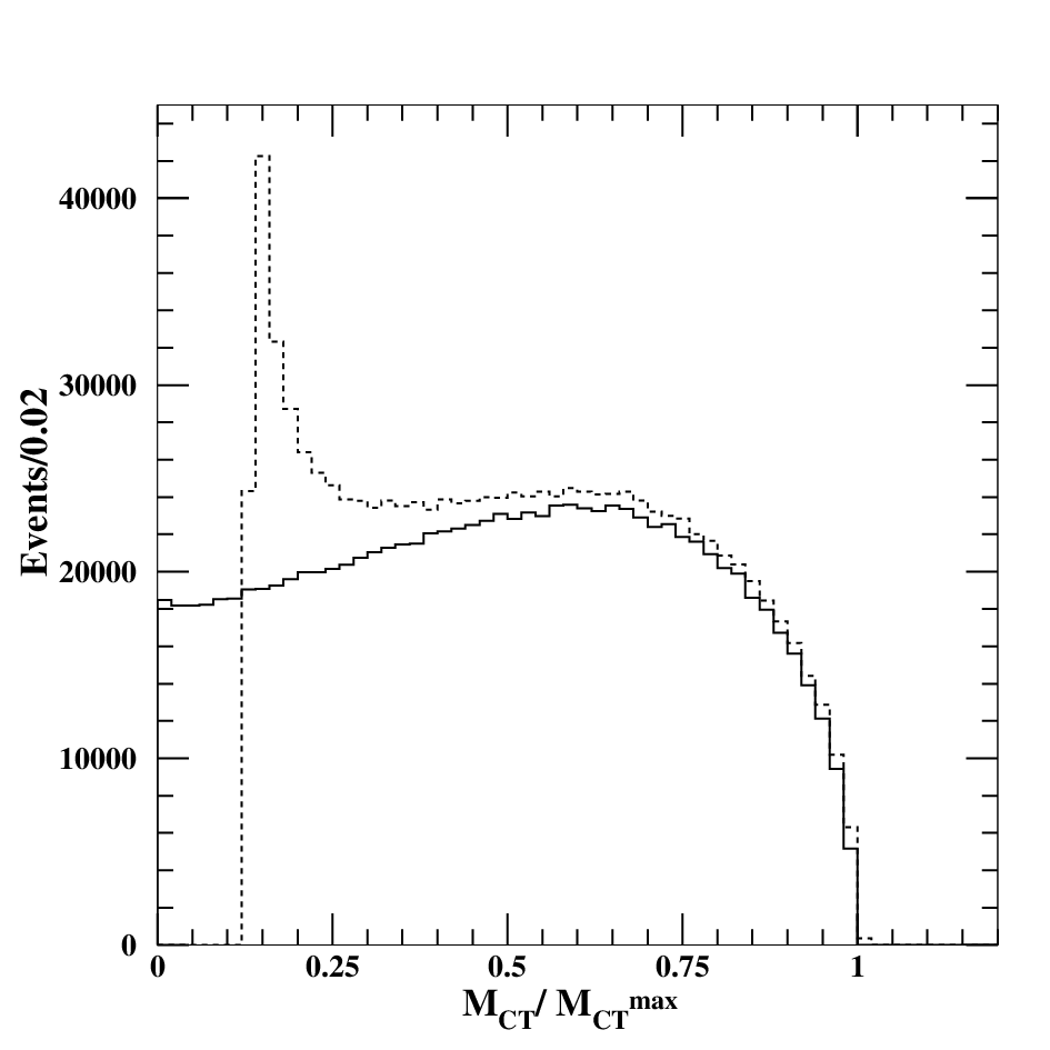
Despite this cancellation of the peak at the distribution can still possess a Jacobian peak. The peak occurs however at the lower limit of the distribution, where (see Eqn. (1)). The distribution tends asymptotically in the absence of boosts to
| (15) |
where is a constant. This is very similar to the functional form of the Jacobian peak, although in this case it is reversed such that the distribution is real above the peak rather than below it. Physically the peak occurs because when the value of becomes independent of the kinematics of and , because the terms in Eqn. (1) dominate. Hence all kinematic configurations generate similar values of . An example of such a peak can be seen in the dashed histogram in Figure 5. Note that when the numerator and denominator in Eqn. (15) cancel leaving a uniform distribution (see e.g. full histogram in Figure 5).
Consider now the general case where the system has been boosted in the laboratory transverse plane, and the boost correction procedure discussed in Section 2.2 has been applied. In this case there can be a further enhancement of the population of events at . If and then the boost-corrected value of is given by from Eqn. (10). If the tranverse momenta of the two visible particles under consideration are bisected by the boost direction however, then can take very small values, even if the transverse momenta of the particles are relatively large. This effect is particularly striking when , in which case it is straight-forward to see from Eqn. (10) that . We shall refer below to the resulting peak at as the ‘’ peak.
Specific examples of the peaks and end-points discussed in this section can be seen in Section 5 below.
4 Measuring and independently
The dependence of on , noted in Ref. [9], and on , noted in Section 2.2, provides potential techniques for measuring and independently. In this section we develop these techniques in more detail.
4.1 Using the dependence of
As remarked in Section 1, when attempting to measure and independently using Eqn. (4) the requirement reduces significantly the event selection efficiency. One can consider ameliorating this problem by removing this mass equality requirement and considering the dependence of the resulting end-point on both and . This is given by
| (16) |
where
| (17) |
In this case all events passing background rejection cuts are used, however the implicit requirement of binning in both and to measure still limits the available event statistics in each end-point measurement (modulo the symmetry under interchange of and of ). As an aside, Eqn. (16) provides a link between the ‘stransverse mass’ [1] and . This is discussed in more detail in Appendix A.
An alternative to using Eqn. (16) for measuring and independently involves observing that is linearly dependent on in Eqn. (4) and hence that
| (18) |
where,
| (19) |
Then we can make use of the following inequality:
| (20) |
to find that
| (21) |
Consequently if the two-dimensional distribution of event values versus event values is plotted, for all events passing background rejection cuts, the distribution will display an end-point dependence on given by:
| (22) |
Hence and may be obtained by measuring the gradient and intercept of the end-point dependence on in a similar manner to the existing technique using Eqn. (4). Now however all events passing the background rejection cuts can be used rather than just a small subset.
It should be noted here that although this technique is sound from a theoretical point-of-view, the uneven distribution of events in the versus plane can cause difficulty when attempting to use it in practice. This is discussed further in Section 5.
4.2 Using the dependence of
In Section 2.2 we developed a procedure for correcting such that it is always bounded from above by the expression for obtained when the upstream momentum . Given sufficient statistics however an alternative procedure would involve binning the non-boost-corrected value of in and measuring and independently from the dependence of on . When this dependence is given by Eqn. (8), however we can also obtain a general expression valid even when , which is
| (23) |
where is obtained from Eqn. (16), , is given by Eqn. (17) and . In principle the additional dependence of on the angle between the vector and the net momentum of and in the transverse plane could also be exploited, although this is not considered further here.
The advantage of using the dependence of rather than the dependence discussed in Section 4.1 is that and can in principle be measured independently even when , for instance when the particles are jets or leptons. This avoids potential combinatorial problems inherent in the latter technique. In this special case the expression for becomes
| (24) |
A toy Monte Carlo example versus distribution for massless particles is shown in Figure 6 together with the theoretical bound from Eqn. 24.

5 Mass measurement for two-step decay chains
5.1 Generic strategy
We shall now investigate the use of the boost-corrected contransverse mass discussed in Section 2.2 (hereafter referred to simply as ) to measure the masses of pair-produced heavy particles decaying via symmetric two-step sequential two-body decay chains. As discussed in Ref. [14] mass measurement with such chains is non-trivial because they are too short to solve fully for the masses using invariant mass end-point techniques [20, 21, 22, 23, 24] or the ‘mass relation’ method [25]. The decay chains considered can be written in the form:
| (25) |
where , and are generic massive particles, and are generic visible particles (here assumed massless) and is invisible. The two chains present in each event can be seen in diagrammatic form in Figure 7, where particles appearing in the second decay chain are denoted with primed labels. We assume in the following discussion that particles labeled with the same letter possess the same mass.
With each event we can construct one pair of invariant mass observables and three contransverse mass observables from the momenta of the four observed particles , , and . These observables are:
- •
: the invariant masses of the visible products of the two decay chains
- •
: constructed from the momenta of and
- •
: constructed from the momenta of and
- •
: constructed from the momenta of the aggregate products of each chain and .
These observables possess kinematic end-points whose positions are functions of the masses , and . The end-point positions are respectively33 3 When dealing with single-step three-body decay chains in which two visible particles and one invisible particle are produced in each decay Eqns. (26)–(29) are replaced by , and , although in the last two cases the distributions are strongly phase-space suppressed near the endpoints.:
| (26) | |||||
| (27) | |||||
| (28) | |||||
| (29) |
where the final relationship is obtained from Eqn. (4) with . In addition the two-dimensional distribution of events in the versus plane discussed in Section 4.1 can be constructed, providing additional mass constraints via Eqn. (22). The two-dimensional distributions of events in the (non-boost-corrected) versus and versus planes discussed in Section 4.2 can also in principle be used.

Using Eqns. (26), (27) and (28) the mass of the parent particle can be calculated from:
| (30) |
The masses of and can then be obtained by simple substitution into Eqns. (27) and (28) respectively. The constraints on the masses provided by Eqn. (22), Eqn. (29) and/or Eqn. (23) may be more difficult to exploit, as shall be discussed in Section 5.2, but they can be used as a closure test for the masses measured using the other constraints.
In typical SUSY decay chains we consider cases where the particles and can be either quarks/jets () or leptons (), leading to the following possible final-state configurations: , and . The second of these configurations is particularly favourable from an experimental point-of-view because in this case there is no ambiguity in assigning particles to steps in the decay chains when constructing and . In the case-studies presented below we shall therefore focus on events with the final state and .
5.2 Benchmarking on top events
The mass measurement technique proposed above can be tested with events in which both top quarks decay to leptons via leptonically decaying ’s through the chain:
| (31) |
Such events contain two symmetric two-step sequential two-body decay chains, with invisible particles being produced at the end of each chain. They therefore provide a suitable testbed for our mass measurement technique, with , , , and . The main notable difference between these events and SUSY events is that the invisible particles are in reality approximately massless, however in our analysis we shall not make this assumption. This approach has been used previously to study alternative SUSY particle mass measurement techniques [18, 14].
In order to evaluate the observables discussed in Section 5.1, we generated with MC@NLO 3.3 [26, 27] an inclusive sample of TeV LHC events with an input top mass of 172.5 GeV. The events were passed through the parameterised detector simulation ACERDET [28] which was modified to reproduce the resolutions for leptons and jets given in [29]. For the tagging of -jets, an efficiency of 60% was assumed, for a light jet rejection of 100. The total generated sample was 2.2 M events, corresponding to an integrated luminosity of approximately 3 fb-1.
Events were selected with the following requirements:
- 1.
2, with 40 GeV
- 2.
30 GeV
- 3.
2, where (isolated) and 20 GeV
- 4.
At least two jets tagged as with GeV
- 5.
Only one of the two possible sets of pairings of the two leptons with the two leading -jets should generate invariant mass values which are both less than 175 GeV. This cut was intended to reduce the experimental combinatorial background and was used only when constructing observables which required the pairing of leptons and jets from the same decay chain.
Approximately 16100 (8300) events passed cuts 1-4 (1-5) respectively. Of these 15200 (7400) were indeed events in which both hard ’s decayed into a muon or electron. The remaining events contained at least one tau lepton decaying leptonically into or .
With the two pairs, each corresponding to the decay of a different top quark, one can construct the observables discussed in Section 5.1. These observables are , , and . Neglecting the mass of the -quark, the end-points in the distributions of these quantities lie at (from Eqns. (26)–(29)):
| (32) | |||||
| (33) | |||||
| (34) | |||||
| (35) |
Accounting for translates into shifts of less than in the end-point positions.
We show in Figure 8 the distributions of the observables at parton-level and at detector-level for events passing the selection cuts in which both ’s decay into electron and muons. All contransverse mass observables have been corrected for transverse boosts according to the procedure discussed in Section 2.2. It can be seen that the end-point structures at parton-level are conserved at detector-level, modulo some smearing. The enhancement observed at the lower limit of the distribution is generated by the Jacobian peak at discussed in Section 3 together with the effect of the boost correction procedure discussed in the same ssection. The distribution in Figure 8 is relatively unaffected by the Jacobian enhancement because for massless leptons. The dilepton systems in these events receive large boosts from the recoil however and so the boost correction procedure generates a prominent peak at .


In order to explore in an approximate manner the potential precision of mass measurements obtained with this technique, we fit the end-points of the distributions with a linear function smeared by detector resolution effects. Following Ref. [29] we use a function given by:
| (36) |
Here is the observable under consideration, represents the end-point position, represents the resolution of the assumed gaussian detector smearing, is the slope of the distribution before smearing, and and are parameters describing an assumed linear background distribution. The latter distribution helps to take into account the effects of both combinatorial background from incorrect assignment of visible particles to decay chains and non-gaussian tails in the experimental resolution.


For the observables and , the fits to the distributions for all detector-level events passing the cuts are shown in Figure 9, with the irreducible background of events where at least one of the leptons is not directly produced in a decay shown in grey (red). The fit function reproduces well the observed shape, and the value of the resolution parameter obtained from the fit is in good agreement with the actual value of the smearing used in the detector simulation.
The situation is somewhat more complex for the observable. In this case one has two populations. If only a very small transverse boost correction is applied to , using . Therefore the experimental end-point resolution is to a good approximation just the resolution of the lepton measurement (of order 1 GeV), plus the end-point smearing arising from the natural width (of order 2-3 GeV). If however, is corrected using the of the hadronic recoil, resulting in a significantly larger resolution of order 9-10 GeV. The two configurations must therefore be fitted separately. The distributions are shown in Figure 10, for () on the left (right). From the figure one can also observe that the gradient of the distribution near the end-point is smaller, and it was necessary in this case to fix the experimental resolution to 3 GeV in order to obtain an acceptable fit.

Measurement of the end-point in the distribution presents further challenges due to the concave shape of the distribution near to the end-point, seen in Figure 8(top-right). For this end-point the assumption of a linear shape breaks down, primarily due to the depopulation of the versus plane near seen in Figure 11. An alternative strategy for constraining the masses with would be to measure the dependence of on , as discussed in Section 4.1. This could be accomplished in practice by constructing histograms of those events which pass a cut on . Unfortunately however this procedure is also complicated by the presence of concave end-points, as can be seen in Figure 12. Further progress with this specific element of the contransverse mass technique will likely require a dedicated study of end-point shapes, which is outside of the scope of this paper. Because of these considerations we will not use the measurements of in the following mass measurement study. Nevertheless such constraints could be useful for validating mass measurements obtained from the other observables. Similar considerations apply when attempting to use the non-boost-corrected and observables to measure the dependence of and on , as shown in Figure 13, and this technique will also not be considered further here.


The results of the end-point fits are listed in Table 1, where the first uncertainty is the statistical uncertainty from the MINUIT [30] fitting program for the chosen fit interval, the second is the systematic uncertainty obtained by varying the fit interval and the third uncertainty is the correlated systematic uncertainty derived from assumed energy scale uncertainties of 1% for -jets and 0.1% for leptons [31]. The quoted uncertainties should be considered approximate and could be improved with the use of better end-point fitting functions, for instance templates derived from Monte Carlo simulation studies.
| End-point | Truth (GeV) | Measured (GeV) |
|---|---|---|
| 152.6 | ||
| 135.0 | ||
| 80.4 | ||
| 80.4 |
Based on the end-point measurement uncertainties listed in Table 1 it is possible to evaluate the achievable precisions for measuring the masses of the top quark, and neutrino. We use the technique described in Ref. [32], where for each end-point measurement we generate a set of pseudo-experiments by sampling from a gaussian distribution centred on the nominal value of the end-point position of width equal to the estimated measurement precision. We assume that the measurements are uncorrelated with the exception of the energy scale uncertainties, which are assumed to be fully correlated. For each pseudo-experiment we calculate the value of according to Eqn. (30) and hence calculate and from Eqns. (33) and (34).

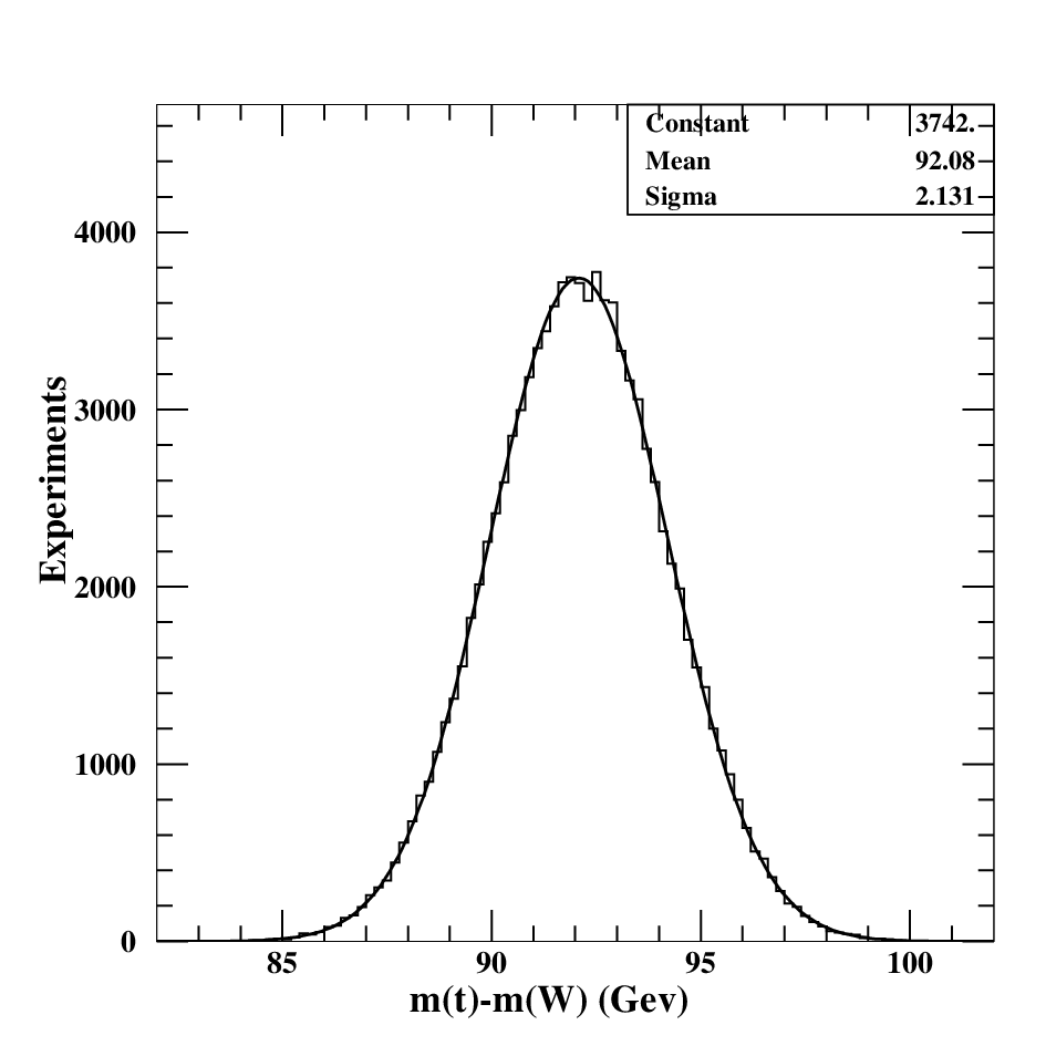
The distributions of the measured values and mass differences are shown in Figure 14 for a set of 100000 pseudo-experiments. The precision of the top quark mass measurement is 8 GeV, while the uncertainty on the measurement of is 2 GeV. A 95%(68%) upper limit on the neutrino mass of 30(16) GeV is obtained. These results may appear to be disappointing when compared with the 1 GeV precision expected to be obtained at the LHC from semileptonic events for the same assumptions on -jet energy scale uncertainty [29]. Here however we have made no assumptions about the masses of the or neutrino and so 8 GeV is the stand-alone precision with can be obtained with the technique. The end-point measurements used in this technique are primarily sensitive to mass differences and so if the mass of the were assumed to be known the precision of the measurement of would improve to 2 GeV, dominated by the systematics associated with the very crude end-point fitting function used for this study.
5.3 A SUSY example
Having demonstrated the proposed mass measurement technique with events let us now apply the same technique to a SUSY model generating events with a similar final state. An example of such a SUSY model is an MSSM model with a left-handed slepton doublet lighter than the chargino. In this case events with the decay chain
| (37) |
appearing in both legs of the event can be produced. The invisible sparticle at the end of the chain is in this case the sneutrino, since both of its decay products are undetected. This decay chain maps onto Eqn. (25) with , , , and .
The decay (37) is however not the only decay yielding the final state of interest, with a quark, a lepton and one or more invisible particles on each leg. We consider the following decay chains:
| (38) | |||||
| (39) | |||||
| (40) |
For all of these decays, formulas (26)–(29) are valid, provided that in (26), (28) and (29) is replaced by , defined as the minimum mass of the “pseudo-particle” composed of all of the invisible particles in the decay. Analytical expressions for in terms of the masses of the particles involved in the decays are given in Appendix B. These can be used in Eqns. (26) and (29).
The case of Eqn. (28) deserves special comment. In this case for decay chains (38), (39) and (40) one invisible particle is upstream of the lepton and one downstream. It is therefore not possible to correct for the upstream momentum, since it is not possible to separate the momentum of the neutrino and of the . However, if one performs the boost correction assuming that all of the observed missing transverse momentum is downstream of the lepton, the distributions for still possess end-points at positions given by Eqn. (28) with the values defined in Appendix B.
Based on measurements of the end-point positions , and , one can calculate the masses of the squark and of the chargino independently from the decay mode of the . This is a remarkable achievement, as it shows that it is possible to perform an absolute measurement of the chargino mass through its leptonic decay notwithstanding the fact that two invisible sparticles are present in the decay of each chargino. The interpretation of the meaning of the measured is dependent on the chargino decay mode, and the analysis based on the measurement of , , and does not allow the discrimination of the different expressions given in Appendix B.
It should be noted that the mass hierarchy and coupling structure implied by the presence of the decay chain given by Eqn. (37) imply also the existence, with a significant branching ratio, of the chain:
| (41) |
which can be easily selected by requiring the presence of two leptons with the same flavour and opposite sign. This ‘golden channel’ for SUSY mass measurement at the LHC can potentially provide additional information regarding the masses of sparticles involved in the chargino decay chain. In the following we shall not show a complete analysis along these lines, which has been already developed in detail in e.g. Refs. [20, 21, 3]. We shall limit ourselves instead to showing for our example model that the invariant mass of two OS-SF leptons does give a characteristic end-point structure from the decay. Starting from this end-point, and combining it with the hard jets in the events it is possible to measure the masses of , and [20, 21, 3]. It is then straightforward to insert the measured values of these masses into Eqns. (26)–(29) and observe that under the assumption of decays (38), (39), and (40) the mass measurements from the two analyses are inconsistent.
In order to explore the feasibility of this measurement technique, we used HERWIG 6.5 [33, 34] to generate events from a toy MSSM model incorporating the mass hierarchy present in decay chain (37). The masses of all of the squarks were set to 500 GeV and those of all the sleptons to 150 GeV. The three gaugino masses , and were set respectively to 120, 250 and 520 GeV while the higgsino mass parameter was set to 400 GeV, to 10, and to 400 GeV. The trilinear couplings were set to zero. The relevant sparticle masses, as calculated by ISASUSY 7.75 [35] are listed in Table 2. The expected end-point positions for the chains (37) and (38) are listed in Table 3, using the results of the discussion above regarding the treatment of in decay chain (38).
| Parameter | Value (GeV) | Parameter | Value (GeV) |
|---|---|---|---|
| 520.0 | 503.4 | ||
| 157.1 | 135.7 | ||
| 231.5 | 232.0 | ||
| 117.2 |
| End-point | Position: Chain (37) | Position: Chain (38) |
|---|---|---|
| 362.1 | 297.7 | |
| 396.9 | 396.9 | |
| 151.9 | 69.7 | |
| 727.2 | 668.5 |
A total of 800 K events were generated, corresponding to an integrated luminosity of 12 fb-1. The generated events were passed through the same parameterised detector simulation as for the top sample described in Section 5.2. Events were selected with the following requirements:
- 1.
2, with 100 GeV and 50 GeV.
- 2.
100 GeV.
- 3.
2, where (isolated) and 20 GeV. The two leptons were required to possess different flavours.
- 4.
Veto all events with jets with 20 GeV labelled as a -jet or -jet.
The veto on and labelled jets was applied to reduce the SUSY background from events containing top quark or lepton decays.
The requirement of leptons with different flavour reduces the signal by a factor two, but it is necessary, as the same-flavour signal is dominated by SUSY background events in which the two leptons are produced in the decay chain (41). This is demonstrated in Figure 15 which shows the lepton-lepton invariant mass distribution for opposite-sign same-flavour lepton pairs. The full line is the inclusive distribution, and exhibits the characteristic end-point structure from decay (41) [20]; the grey (red) area indicates lepton pairs from the decays (37) and (38). Figure 15 demonstrates also that the characteristic lepton-lepton invariant mass end-point from the decay chain is indeed observable for this model.

Following application of the selection cuts described above the only significant remaining background was from production and only this background is considered in the following. Approximately 9700 SUSY events passed cuts 1–4. Of these 7200 were indeed events in which both the muon and the electron were produced directly in the decay of a sparticle from the chains (37) or (38). In the remaining events at least one of the leptons was generated by the decay of a tau lepton produced in one of the two legs of the event. The number of background events was approximately 1400.
The parton-level distributions for the observables , , and are shown in Figure 16 for all events passing the selection cuts in which both legs in the event contain the chain (37) or the chain (38). The contransverse mass observables have been corrected for transverse boosts according to the procedure described in Section 2.2. For the reasons discussed in Section 5.2 we shall not measure or exploit the end-points in the following analysis, nor the non-boost-corrected and versus end-points. Nevertheless such constraints could be useful for validating mass measurements obtained from the other observables.


The first step in the detector-level analysis is the calculation of the invariant mass of each lepton with each of the two leading jets in the event. The distribution of the minimum of these two masses for each lepton is plotted in Figure 17 and displays an end-point at around 360 GeV, as expected from chain (37). The detector-level distributions of and are plotted in Figure 18 and also display end-points at the positions expected for chain (37). Only the distribution of values for events with is shown. This is due to the fact that the distribution at truth level for hits the nominal end-point, whereas that for runs out of statistics approximately 10 GeV below the nominal position (see Figure 19(left)), leading to a biased fitted end-point position at detector level (see Figure 19(right)). This arises because only a very small boost correction (with ) can be applied in the case and hence the resulting corrected value is more conservative than in the case. This effect is most evident when considering because of the potentially large boosts generated by the recoiling system. The same effect, although numerically less evident, is present also in the top quark analysis but is masked by the smearing of the end-point due to the natural width. We choose here to use the larger of the two fitted end-point positions, which must be nearer to the true value.


In order to explore the approximate potential precision of mass measurements obtained with this technique, we fit the end-points of the distributions with the smeared linear function given in Eqn. (36). The caveats associated with this technique discussed in Section 5.2 are also relevant here. In the case of the distribution we only fit the distribution of events with , as discussed above. The fitted distributions are shown in Figures 17 and 18.
| End-point | Truth (GeV) | Measured (GeV) |
|---|---|---|
| 362.1 | ||
| 396.9 | ||
| 151.9 |
The results of the end-point fits are listed in Table 4, where the first uncertainty is the statistical uncertainty from the MINUIT [30] fitting program for the chosen fit interval, the second is the systematic uncertainty obtained by varying the fit interval and the third uncertainty is the correlated systematic uncertainty derived from assumed energy scale uncertainties of 1% for jets and 0.1% for leptons [31]. As for the top study the quoted uncertainties should be considered approximate and could be improved with the use of better end-point fitting functions, for instance templates derived from Monte Carlo simulation studies.
If we use the measured end-point positions to calculate the masses of the sparticles using Eqns. (30), (27) and (28) we obtain an uncertainty of 20 GeV on the absolute squark mass, an uncertainty of 6 GeV on the difference between the squark mass and the masses of the other sparticles, and an uncertainty of 3 GeV on the chargino-sneutrino mass difference. We have thus shown with a toy SUSY model that it is possible to achieve a stand-alone measurement of sparticle masses using the contransverse mass technique applied to events containing two symmetric sequential two-step two-body decay chains.
6 Conclusions
In this paper we have extended the contransverse mass technique for measuring the masses of pair-produced semi-invisibly decaying heavy particles so that it can be applied to events with non-negligible boosts of the CoM frame of the heavy states in the laboratory transverse plane. We have demonstrated the modified technique with case studies measuring the masses of the top quark, and neutrino in fully leptonic events, and the masses of sparticles in SUSY events with a similar final state. The case studies presented here are in many respects more detailed than previous studies of alternative strategies and illustrate well the potential utility of the contransverse mass technique.
Acknowledgements
The authors wish to thank Mihoko Nojiri and Alan Barr for helpful comments. DRT wishes to acknowledge STFC and the Leverhulme Trust for support.
Note added to version 2: Since version 1 of this paper was released onto arXiv a paper [38] has been released which also derives Eqn. (24). The boost-dependence study described in Section 4.2, which appeared in version 2 of this paper, was carried out without knowledge of Ref. [38], however we are happy to acknowledge that Eqn. (24) appeared in Ref. [38] first.
Appendix A The connection between and
Eqn. (16) can be used to study the links between [1] and , as we shall now illustrate. In the process we shall obtain an approximate analytical expression for a boost-corrected version of . The link between the two quantities in the absence of co-linear transverse boosts and for massless visible states was first discussed in Ref. [36].
First, observe that if we assume a value for and know then we can solve Eqn. (16) for . For any given event we do not know however, but rather . Let us therefore substitute for to obtain the following solution
| (A1) |
where and is the assumed value of . This is identical to the analytical expression for the ‘balanced’ solution of in the absence of co-linear transverse boosts, which was identified in Refs. [37, 7]. In general need not be bounded by , because and hence appears in the denominator inside the square-root causing not to be a monotonically increasing function of . Therefore a value of need not generate a value of which is less than the value obtained with . Note that if then is nevertheless bounded by because in this special case is a monotonically increasing function of .
In general is not invariant under co-linear transverse boosts, because it depends on which is also not invariant. One might consider therefore whether it is possible to correct for such boosts in a similar manner to that used to correct in Section 2.2. The boost-correction procedure minimises with respect to the possible boosts, however this does not necessarily minimise because it is not in general a monotonically increasing function of . Boost-correction can be performed however, as we know not only the minimum possible value of in the CoM frame but also the maximum possible value, which is given by the maximum of the values obtained by boosting and with respectively and (see Fig. 3). We therefore know the range of CoM frame values which could have occurred in the event.
To proceed we find the turning-points of Eqn. (A1), which lie at the following four values of :
| (A2) |
where . We then take the minimum of all the values obtained at turning-points where lies within the allowed range identified above. We finally take the minimum of this value and those obtained with set to its extrema. The result is a boost-corrected value of .
Now although is not in general bounded by the full analytical expression for in the absence of co-linear transverse boosts [37, 7] is so bounded. This is because in those cases where takes on an alternative value corresponding to an ‘unbalanced’ solution (see e.g. Eqn. (54) in Ref. [37]). The quantities upon which the decision to switch to such an alternative value rests are not themselves boost-invariant. Development of an appropriate boost-correction procedure for these quantities consistent with the parallel boost-correction of requires more work. In the absence of such a correction procedure we can choose to neglect the boost when making this decision, to obtain an approximate analytical form for a boost-corrected version of .
Note that the quantity calculated here is not the same quantity as the conventional used elsewhere, which is boost-independent but currently does not possess a general analytical form. The boost-correction procedure, even if exact (i.e in the absence of the approximation mentioned in the previous paragraph), leads to a quantity which is not in general equal to the conventional , although equality is obtained in the absence of co-linear transverse boosts.
The procedure described above for calculating this ‘boost-corrected ’ quantity is implemented in the boost-correction package described in Section 2.2, available at http://projects.hepforge.org/mctlib.
Appendix B Invisible pseudo-particle masses for chargino decay chains
If a heavy sparticle decays via a chain which produces multiple invisible final state particles then the values of and can be calculated by constructing an aggregate ‘pseudo-particle’ from the invisible particles. The minimum value of , , can then be used in end-point formulae, as described in Section 5.3.
If a chargino decays through then and is given by:
| (B1) |
where
| (B2) | |||||
| (B3) | |||||
| (B4) |
and we have assumed . If however the chargino decays through , as in decay chain (38), then:
| (B5) |
while if the chargino decays through , as in decay chain (37), then and is fixed to given by:
| (B6) |
Finally, if the chargino decays through the three-body decay then and is given by:
| (B7) |
References
- [1] C. G. Lester and D. J. Summers, Phys. Lett. B 463 (1999) 99 [arXiv:hep-ph/9906349].
- [2] A. Barr, C. Lester and P. Stephens, J. Phys. G 29 (2003) 2343 [arXiv:hep-ph/0304226].
- [3] B.K. Gjelsten, J. Hisano, K. Kawagoe, E. Lytken, D. Miller, M. M. Nojiri, P. Osland and G. Polesello in G. Weiglein et al. [LHC/LC Study Group], Phys. Rept. 426 (2006) 47 [arXiv:hep-ph/0410364].
- [4] W. S. Cho, K. Choi, Y. G. Kim and C. B. Park, Phys. Rev. Lett. 100 (2008) 171801 [arXiv:0709.0288 [hep-ph]].
- [5] B. Gripaios, JHEP 0802 (2008) 053 [arXiv:0709.2740 [hep-ph]].
- [6] A. J. Barr, B. Gripaios and C. G. Lester, JHEP 0802 (2008) 014 [arXiv:0711.4008 [hep-ph]].
- [7] W. S. Cho, K. Choi, Y. G. Kim and C. B. Park, JHEP 0802 (2008) 035 [arXiv:0711.4526 [hep-ph]].
- [8] M. M. Nojiri, Y. Shimizu, S. Okada and K. Kawagoe, JHEP 0806 (2008) 035 [arXiv:0802.2412 [hep-ph]].
- [9] D. R. Tovey, JHEP 0804 (2008) 034 [arXiv:0802.2879 [hep-ph]].
- [10] A. J. Barr, G. G. Ross and M. Serna, Phys. Rev. D 78 (2008) 056006 [arXiv:0806.3224 [hep-ph]].
- [11] M. M. Nojiri, K. Sakurai, Y. Shimizu and M. Takeuchi, JHEP 0810 (2008) 100 [arXiv:0808.1094 [hep-ph]].
- [12] W. S. Cho, K. Choi, Y. G. Kim and C. B. Park, Phys. Rev. D 79 (2009) 031701 [arXiv:0810.4853 [hep-ph]].
- [13] H. C. Cheng and Z. Han, JHEP 0812 (2008) 063 [arXiv:0810.5178 [hep-ph]].
- [14] M. Burns, K. Kong, K. T. Matchev and M. Park, JHEP 0903 (2009) 143 [arXiv:0810.5576 [hep-ph]].
- [15] A. J. Barr, A. Pinder and M. Serna, Phys. Rev. D 79 (2009) 074005 [arXiv:0811.2138 [hep-ph]].
- [16] K. T. Matchev, F. Moortgat, L. Pape and M. Park, arXiv:0909.4300 [hep-ph].
- [17] CDF Collaboration, CDF Note 9679.
- [18] W. S. Cho, K. Choi, Y. G. Kim and C. B. Park, Phys. Rev. D 78 (2008) 034019 [arXiv:0804.2185 [hep-ph]].
- [19] A. J. Barr, JHEP 0602 (2006) 042 [arXiv:hep-ph/0511115].
- [20] H. Bachacou, I. Hinchliffe and F. E. Paige, Phys. Rev. D 62 (2000) 015009 [arXiv:hep-ph/9907518].
- [21] B. C. Allanach, C. G. Lester, M. A. Parker and B. R. Webber, JHEP 0009 (2000) 004 [arXiv:hep-ph/0007009].
- [22] D. Costanzo and D. R. Tovey, JHEP 0904 (2009) 084 [arXiv:0902.2331 [hep-ph]].
- [23] M. Burns, K. T. Matchev and M. Park, JHEP 0905 (2009) 094 [arXiv:0903.4371 [hep-ph]].
- [24] K. T. Matchev, F. Moortgat, L. Pape and M. Park, JHEP 0908 (2009) 104 [arXiv:0906.2417 [hep-ph]].
- [25] K. Kawagoe, M. M. Nojiri and G. Polesello, Phys. Rev. D 71 (2005) 035008 [arXiv:hep-ph/0410160].
- [26] S. Frixione and B. R. Webber, JHEP 0206 (2002) 029 [arXiv:hep-ph/0204244].
- [27] S. Frixione, P. Nason and B. R. Webber, JHEP 0308 (2003) 007 [arXiv:hep-ph/0305252].
- [28] E. Richter-Was, arXiv:hep-ph/0207355.
- [29] The ATLAS Collaboration, “Expected Performance of the ATLAS Experiment, Detector, Trigger and Physics” CERN-OPEN-2008-020 (2008).
- [30] F. James and M. Roos, Comput. Phys. Commun. 10 (1975) 343.
- [31] ATLAS Collaboration, ATLAS detector and physics performance Technical Design Report, CERN/LHCC 99-14/15 (1999).
- [32] M. M. Nojiri, G. Polesello and D. R. Tovey, JHEP 0603 (2006) 063 [arXiv:hep-ph/0512204].
- [33] G. Corcella et al., JHEP 0101 (2001) 010 [arXiv:hep-ph/0011363].
- [34] S. Moretti, K. Odagiri, P. Richardson, M. H. Seymour and B. R. Webber, JHEP 0204 (2002) 028 [arXiv:hep-ph/0204123].
- [35] F. E. Paige, S. D. Protopopescu, H. Baer and X. Tata, arXiv:hep-ph/0312045.
- [36] M. Serna, JHEP 0806 (2008) 004 [arXiv:0804.3344 [hep-ph]].
- [37] C. Lester and A. Barr, JHEP 0712 (2007) 102 [arXiv:0708.1028 [hep-ph]].
- [38] K. T. Matchev and M. Park, arXiv:0910.1584 [hep-ph].