Spin motive forces and current fluctuations due to Brownian motion of domain walls
Abstract
We compute the power spectrum of the noise in the current due to
spin motive forces by a fluctuating domain wall. We find that the
power spectrum of the noise in the current is colored, and depends
on the Gilbert damping, the spin transfer torque parameter
, and the domain-wall pinning potential and magnetic
anisotropy. We also determine the average current induced by the
thermally-assisted motion of a domain wall that is driven by an
external magnetic field. Our results suggest that measuring the
power spectrum of the noise in the current in the presence of a
domain wall may provide a new method for characterizing the
current-to-domain-wall coupling in the system.
Keywords: A. Magnetically ordered materials; A. Metals; A.
Semiconductors; D. Noise
Pacs numbers: 72.15 Gd, 72.25 Pn, 72.70 +m
1 Introduction
Voltage noise has long been considered a problem. Engineers have been concerned with bringing down noise in electric circuits for more than a century. The seminal work by Johnson[1] and Nyquist[2] on noise caused by thermal agitation of electric charge carriers (nowadays called Johnson-Nyquist noise) was largely inspired by the problem caused by noise in telephone wires. The experimental work by Johnson tested the earlier observations by engineers that noise increases with increasing resistance in the circuit and increasing temperature. He was able to show that there would always be a minimal amount of noise, beyond which reduction of the noise is not possible, thus providing a very practical tool for people working in the field. At the same time, the theoretical support for these predictions was given by Nyquist. It is probably not a coincidence that, at the time of his research, Nyquist worked for the American Telephone and Telegraph Company.
As long as noise is frequency-independent, i.e., white like Johnson-Nyquist noise, it is indeed often little more than a nuisance (a notable exception to this is shot noise[3] at large bias voltage). However, frequency-dependent, i.e., colored noise can contain interesting information on the system at hand. For example, in a recent paper Xiao et al.[4] show that, via the mechanism of spin pumping[5], a thermally agitated spin valve emits noisy currents with a colored power spectrum. They show that the peaks in the spectrum coincide with the precession frequency of the free ferromagnet of the spin valve. This opens up the possibility of an alternative measurement of the ferromagnetic resonance frequencies and damping, where one does not need to excite the system, but only needs to measure the voltage noise power spectrum. Here, we see that properties of the noise contain information on the system. Clearly, this proposal only works if the Johnson-Nyquist noise is not too large compared to the colored noise.
Not only precessing magnets in layered structures induce currents: Recent theoretical work has increased interest in the inverse effect of current-driven domain-wall motion, whereby a moving domain wall induces an electric current[6, 7, 8, 9]. Experimentally, this effect has been seen recently with field-driven domain walls in permalloy wires[10]. These so-called spin motive forces ultimately arise from the same mechanism as spin pumping induced by the precessing magnet in a spin valve, i.e., both involve dynamic magnetization that induces spin currents that are subsequently converted into a charge current.
In this paper, we study the currents induced by domain walls at nonzero temperature. In particular, we determine the (colored) power spectrum of the emitted currents due to a fluctuating domain wall, both in the case of an unpinned domain wall (Sec. 2.2), and in the case of a domain wall that is extrinsically pinned (Sec. 2.3). We also compute the average current induced by a field-driven domain wall at nonzero temperature. We end in Sec. 4 with a short discussion and, in particular, compare the magnitude of the colored noise obtained by us with the magnitude of the Johnson-Nyquist noise.
2 Spin motive forces due to fluctuating domain walls
In this section, we compute the power spectrum of current fluctuations due to spin motive forces that arise when a domain wall is thermally fluctuating. We consider separately the case of intrinsic and extrinsic pinning.
2.1 Model and approach
The equations of motion for the position and the chirality of a rigid domain wall at nonzero temperature are given by[11, 12, 13]
| (1) | ||||
| (2) |
where is Gilbert damping, is the hard-axis anisotropy, and is the domain-wall width, with the spin stiffness and the easy-axis anisotropy. We introduce a pinning force, denoted by , to account for irregularities in the material. We have assumed that the pinning potential only depends on the position of the domain wall. Pinning sites turn out to be well-described by a potential that is quadratic in , such that we can take [11]. The Gaussian stochastic forces describe thermal fluctuations and are determined by
| (3) |
They obey the fluctuation-dissipation theorem[12]
| (4) |
Note that in this expression, the temperature is effectively reduced by the number of magnetic moments in the domain wall , with the cross-sectional area of the sample, and the lattice spacing. Up to linear order in the coordinate , valid when , we can write the equations of motion in Eqs. (1) and (2) as
| (5) |
where
| (6) |
and
| (7) |
We readily find that the eigenfrequencies of the system, determined by the eigenvalues of the matrix , are
| (8) |
with both the eigenfrequencies and their damping rates real numbers. Their behavior as a function of is shown in Fig. 1.

Note that this expression has an imaginary part for pinning potentials that obey , and, because for typical materials the damping assumes values , the eigenfrequency assumes nonzero values already for very small pinning potentials. Without pinning potential () the eigenvalues are purely real-valued and the motion of the domain wall is overdamped since and .
If we include temperature, we find from the solution of Eq. (5) [without loss of generality we choose ] that the time derivatives of the collective coordinates are given by
| (9) |
for one realization of the noise. By averaging this solution over realizations of the noise, we compute the power spectrum of the current induced by the domain wall under the influence of thermal fluctuations as follows.
It was shown by one of us[8] that up to linear order in time derivatives, the current induced by a moving domain wall is given by
| (10) |
with the length of the sample, and the sum of the phenomenological dissipative spin transfer torque parameter[14] and non-adiabatic contributions. The power spectrum is defined as
| (11) |
Note that in this definition the power spectrum has units , not to be mistaken with the power spectrum of a voltage-voltage correlation, which has units . In both cases, however, the power spectrum can be seen as a measure of the energy output per frequency interval. We introduce now the matrix
| (12) |
so that we can write the correlations of the current as
| (13) |
We evaluate the traces that appear in this expression to find that the power spectrum is given by
| (14) |
2.2 Domain wall without extrinsic pinning
We first consider a domain wall with . In this case, only the chirality determines the energy, a situation referred to as intrinsic pinning[11]. From the result in Eq. (14) we find that the power spectrum is given by
| (15) |
Indeed, we find that next to a constant contribution there is also a frequency-dependent contribution for , i.e., the power spectrum is colored. The fact that is a special case is understood from the fact that in that case we have macroscopic Galilean invariance. This translates to white noise in the current correlations. The power spectrum is a Lorentzian, centered around because the domain wall is overdamped in this case, with a width determined by the damping rate in Eq. (8) as . Relative to the white-noise contribution
| (16) |
the height of the peak is given by . The behavior of the power spectrum is illustrated in Fig. 2 for several values of .

2.3 Extrinsically pinned domain wall
For extrinsically pinned domain walls the behavior of the power spectrum given by Eq. (14) is depicted in Fig. 3.
 |
| (a) |
 |
| (b) |
 |
| (c) |
We see that for the peaks in the power spectrum are approximately centered around the eigenfrequencies , consistent with Eq. (8). We can discern between two regimes, one where in figs. 3 (a-d), and one where in figs. 3 (e-f). In the former regime, the height of the peaks in the power spectrum depend strongly on the pinning. For small we see a clear dependence on the value of , whereas for large this dependence is less significant. In the regime of large , the height of the peaks hardly depends on the pinning and is approximately given by . Note that the width of the peaks is independent of . For pinning potentials the width is given by , so for the dependence of the width on the pinning is negligible.
3 Spin motive forces due to thermally-assisted field-driven domain walls
In this section we compute the average current that is induced by a moving domain wall. The domain wall is moved by applying an external magnetic field parallel to the easy axis of the sample. In this section we take into account temperature but ignore extrinsic pinning (see Ref. [15] for a calculation of spin motive forces in a weakly extrinsically pinned system for ). The equations of motion for a field-driven domain wall are then given by[11, 12, 13]
| (17) | ||||
| (18) |
where is the magnetic field in the z direction, and the stochastic forces are determined by Eq. (3) with the strength given by Eq. (4). In earlier work[13], we computed from these coupled equations the average drift velocity of a domain wall (here, we set the applied spin current zero)
| (19) |
with (we omit factors )
| (20) |
Combining Eqs. (10) and (19) gives us the average current straightforwardly
| (21) |
We evaluate this expression for several temperatures in Fig. 4.
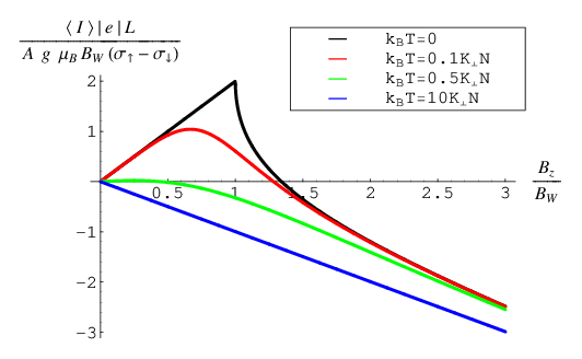
The black curve in Fig. 4 is computed at zero temperature. It increases linearly with the field up to the Walker-breakdown field , where it reaches a maximum current of . Then, it drops and even changes sign. This curve is consistent with the curves obtained by one of us[8]. There, an open circuit is treated where there is no current but a voltage. The voltage is related to the current as , such that indeed , where the normalization is defined as and the polarization is given by . Increasing temperatures smoothen the peak around the Walker-breakdown field, and for high temperatures, the peak vanishes altogether. Therefore, for fields smaller than the Walker-breakdown field and for small temperatures, the thermal fluctuations tend to decrease the average induced current. However, for higher temperatures, the current reverses and increases again. For fields sufficiently larger than the Walker-breakdown field, we always find a slight increase of the current as a function of temperature.
4 Discussion and conclusions
In Sec. 2 we computed power spectra for domain walls, both with and without extrinsic pinning. In ferromagnetic metals, the spin transfer torque parameter has values , for which we see that for large pinning the power spectra only weakly depend on the spin transfer torque parameter . Therefore, determination of is only possible for very small pinning potentials. In an ideally clean sample without extrinsic pinning the height and sign of the peak in the power spectrum can give a clear indication whether is smaller, (approximately) equal or larger than .
In order to perform these experiments, the contributions due to the domain wall should not be completely overwhelmed by Johnson-Nyquist noise. The ratio of the peaks in our power spectrum and the Johnson-Nyquist noise determine the resolution of the experiment, and we want it to be at least of the order of a percent. We use that the resistance of the domain wall is small, and the Johnson-Nyquist noise is governed by the resistance of the wire. For a wire of length and cross-section , the power spectrum due to Johnson-Nyquist noise is given by . From section (2.2) we can estimate the ratio of the height of the peak and the Johnson-Nyquist noise as . To make a rough estimate of this ratio, we use such that for , a polarization and a conductivity . We then find , which shows that the wire length must satisfy in order to have a resolution of 1%. We therefore conclude that this effect at zero pinning is impossible to see in experiment, where wires are typically at least of the order of , i.e., five orders of magnitude larger. We can try to increase the signal by turning on a pinning potential. Insertion of the eigenfrequencies from Eq. (8) in Eq. (14) shows us that we can maximally gain a factor for , as illustrated in Fig. 5.

We can also still gain some resolution by considering a domain wall in a nanoconstriction, where the width can be as small as nm[16]. All this adds up to a resolution of . Therefore, with all parameter values set to ideal values it appears to be possible to observe our predictions in ferromagnetic metals, although the experimental challenges are big.
In a magnetic semiconductor like GaMnAs the number of magnetic moments in the domain wall is two orders of magnitude smaller than in a ferromagnetic conductor. This increases the ratio with a factor . However, the conductivity is also considerably smaller than that in a ferromagnetic metal. The conductivity of GaMnAs depends on many parameters, but a reasonable estimate is that it is at least about three orders of magnitude smaller than that of a metal, although usually even smaller. Therefore, the advantage of a small number of magnetic moments is cancelled. Another property, however, of GaMnAs is that the parameter can assume considerably higher values[17], up to . This does not influence the maximal value of the power spectrum, but it does dramatically increase the value for small pinning.
Note that there are contributions to the noise that we did not discuss in this article. For example, the time-dependent magnetic field caused by a moving domain wall will induce electric currents that contribute to the colored power spectrum. Distinguishing such contributions from the spin motive forces was essential for the experimental results by Yang et al. [10], and would also be important here.
In Sec. 3, we calculated the current induced by a field-driven domain wall under the influence of temperature. We estimate that in ferromagnetic metals at room temperature that , which is indistinguishable from the zero-temperature curve in Fig. 4. However, for magnetic semiconductors, like GaMnAs, we find at , which corresponds to the red curve in Fig. 4. We therefore expect finite-temperature effects to be important in magnetic semiconductors like GaMnAs.
5 acknowledgement
This work was supported by the Netherlands Organization for Scientific Research (NWO) and by the European Research Council (ERC) under the Seventh Framework Program. We would like to thank Yaroslav Tserkovnyak for useful discussions.
References
- [1] J.B. Johnson, Nature 119, 50 (1927); Phys. Rev. 29, 367 (1927); Phys. Rev. 32, 97 (1928).
- [2] H. Nyquist, Phys. Rev. 29, 614 (1927); Phys. Rev. 32, 110 (1928).
- [3] M.J.M. de Jong and C.W.J. Beenakker, in Mesoscopic Electron Transport, edited by L.L. Sohn, L.P. Kouwenhoven and G. Schoen, NATO ASI Series (Kluwer Academic, Dordrecht, 1997), Vol. 345, pp. 225-258.
- [4] J. Xiao, G.E.W. Bauer, S. Maekawa and A. Brataas, Phys. Rev. B 79, 174415 (2009).
- [5] Y. Tserkovnyak, A. Brataas and G.E.W. Bauer, Phys. Rev. Lett. 88, 117601 (2002).
- [6] S.E. Barnes and S. Maekawa, Phys. Rev. Lett. 98, 246601 (2007).
- [7] W.M. Saslow, Phys. Rev. B 76, 184434 (2007).
- [8] R.A. Duine, Phys. Rev. B 77, 014409 (2008); R.A. Duine, Phys. Rev. B 79, 014407 (2009).
- [9] Y. Tserkovnyak and M. Mecklenburg, Phys. Rev. B 77, 134407 (2008).
- [10] S.A. Yang, G.S.D. Beach, C. Knutson, D. Xiao, Q. Niu, M. Tsoi, and J.L. Erskine, Phys. Rev. Lett. 102, 067201 (2009).
- [11] G. Tatara and H. Kohno, Phys. Rev. Lett. 92, 086601 (2004); 96, 189702 (2006).
- [12] R.A. Duine, A.S. Núñez and A.H. MacDonald, Phys. Rev. Lett. 98, 056605 (2007).
- [13] M.E. Lucassen, H.J. van Driel, C. Morais Smith and R.A. Duine, Phys. Rev. B 79, 224411 (2009).
- [14] S. Zhang and Z. Li, Phys. Rev. Lett. 93, 127204 (2004).
- [15] V. Lecomte, S.E. Barnes, J.-P. Eckmann and T. Giamarchi, Phys. Rev. B 80, 054413 (2009).
- [16] P. Bruno, Phys. Rev. Lett. 83, 2425 (1999).
- [17] K.M.D. Hals, A.K. Nguyen and A. Brataas, Phys. Rev. Lett. 102, 256601 (2009).