Non-local dynamics is the hallmark of string theory - the key ingredient for regularizing quantum gravity and providing for a consistent and unified UV completion of particle physics. In recent years, there have been several interesting attempts at zeroing onto this key attribute of the theory in simplified and computationally more accessible regimes. This involves a process of scaling out gravitational complications while retaining the non-local aspects of the parent theory. These attempts have come in several flavors: Non-Commutative Super Yang-Mills (NCSYM) [1]-[5], Non-Commutative Open String (NSOS) theory [6]-[8], Open Membrane (OM) theory [10], Dipole Field (DF) theory [11]-[14], and, most recently, Puff Field theory (PFT) was proposed by Ganor [15, 16, 17]. In all these instances, a decoupling limit is employed to scale out gravity and a flux or geometrical twist is used to tune the scale of the residual non-locality. PFT however stands out in that it can realize non-locality in an $SO(3)$ invariant manner, lending itself to cosmological applications.

To this date, relatively little is understood about PFT. In a recent work [18], a particular realization of a PFT was explored at strong coupling - through the holographic dual description - leading to a myriad of perplexing observations. The system seems to admit a very unusual holographic setup, one that necessitates going beyond the standard dictionary employed, for example, in the AdS/CFT context [19, 20, 21]. [18] focused on cosmological implications of the results. In this work, we focus on the PFT itself, and unravel a surprisingly rich and beautiful holographic dictionary.

On Puff Field Theory

PFT is the worldvolume theory of D-branes in a Melvin universe [15]⁴⁴ 4 For other realizations of branes in Melvin backgrounds, see [22]-[25]. The setup can be realized in numerous different flavors: ones involving D-branes of different dimensionalities and varying amounts of supersymmetry (SUSY). The case we focus on in this paper is $3+1$ dimensional PFT with $\mathcal{N}=2$ SUSY and $U(1)\times U(2)$ R-symmetry, a theory of D3 branes in a Melvin background. The scale of non-locality arises from a single geometrical twist parameter. The theory flows in the IR to $\mathcal{N}=4$ local SYM.

An unusual aspect of this theory is that its spectrum includes non-local states - 3-ball bubbles of size set by the scale of non-locality in the theory. Yet the origin of such states is rather mysterious since there are no open D3 branes in the parent theory. And a Lagrangian description of this PFT is still missing.

In [16], the holographically dual geometry to this PFT was developed, making the strong coupling regime accessible through supergravity computations. The Penrose-Cartan diagram for the bulk spacetime is shown in Figure 1.

We show on this diagram the PFT time coordinate $T$, and the holographic direction $\xi$. A standard UV-IR relation[26] matches high energy with small $\xi$, and low energy with large $\xi$

$$\mu\sim\frac{1}{\xi}$$

(1)

where $\mu$ is energy scale in the PFT. Local operators of the PFT are inserted in the UV, near $\xi=0$, as usual. And all seems holographically normal this far. The novelty arises when one considers operators with certain R-charges that are expected to have non-local features. They are the mysterious D3 bubbles alluded to earlier. In this work, we present a detailed exploration of such states, and find a remarkable holographic mechanism at work.

Summary of the results

R-charge in the PFT is angular momentum in the holographic bulk. In this case, the bulk spacetime carries angular momentum as well, related to the geometrical twist that underlies the non-local character of the PFT. Measuring the R-charge of an operator insertion becomes a delicate matter due to the effects of frame dragging. We show that, whenever the operator is to carry R-charge of a type expected to lead to non-local effects, the insertions would be placed not at the boundary $\xi=0$, but at $\xi=\xi_{0}>0$ inside the bulk - at a shifted holographic screen! To ascertain the reliability of this conclusion, we employ the covariant holographic criterion of Bousso [27]: we look at the rate of convergence of null geodesics projected in the holographic direction $\xi$. We find that this rate vanishes at $\xi=\xi_{0}$. Bousso’s light-sheets are arranged such that the region $\xi>\xi_{0}$ is expected to be holographically encoded at $\xi=\xi_{0}$; while the region $\xi<\xi_{0}$ is also to be encoded on the same surface $\xi=\xi_{0}$.

We then use geodesics to estimate the correlation functions between such non-local operator insertions. We find that the correlators involve a minimum distance scale $\Delta x_{m}$

$$\langle\mathcal{O}(x_{1})\mathcal{O}(x_{2})\rangle\sim\left\{\begin{array}[]{ll}\left(\Delta x\right)^{-4\,h_{+}}&\Delta x\gg\Delta x_{m}\\ e^{-2\,h_{+}\,\left(\frac{\Delta x}{\Delta x_{m}}\right)}&\Delta x\,\widetilde{<}\,\Delta x_{m}\end{array}\right.\$$

(2)

for a bulk probe corresponding to an operator of weight $h_{+}$ in the IR of the theory. We show that $\Delta x_{m}$ corresponds to $\xi\sim\xi_{0}$ through the UV-IR relation, and is also the scale of non-locality in theory - proportional to the geometrical twist of the PFT. We are then led to the holographic dictionary depicted in Figure 2.

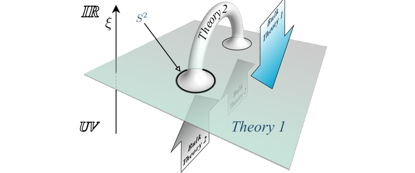
In this Figure, $\xi$ is the vertical direction, and we cartoon the D3 brane worldvolume as a 2D surface. The computation of a two-point correlator of non-local states in the PFT involves a deformation of the worldvolume such that a D3 brane tentacle is projected into the bulk. The operator insertions may be viewed as two 3-balls excised from the worldvolume and joined by the tentacle. The holographic region $\xi>\xi_{0}$ describes the effective theory of interactions of the non-local footprints and may be viewed as projected onto the D3 worldvolume minus the two 3-bubbles. We call this in the Figure ‘Theory 1’.

The region $\xi<\xi_{0}$ on the other hand must describe the degrees of freedom of the tentacle! As seen from the Figure, it employs an IR cutoff related to the size of the 3-bubbles. We compute correlators along the tentacle through geodesics folding into the $\xi<\xi_{0}$ region. We demonstrate that higher energy in Theory 2 corresponds to larger separations between the operator insertions - a direct realization of UV-IR mixing: higher energy corresponds to a longer protrusion. The D3 tentacle may be viewed as the result of an open string pulling on its two endpoints that are attached to the D3 brane worldvolume. In general, we may consider ‘Theory 2’ as the effective theory of such protrusions from the D3 brane worldvolume - states that will necessarily leave a non-local footprint in Theory 1.

In reality, Theory 1 and Theory 2 are coupled, as can be seen from the causal structure of the Penrose-Cartan diagram. The holographic screen at $\xi=\xi_{0}$ that separates the two theories in the bulk is where the convergence rate of null geodesics vanishes: it is a minimal volume neck in the geometry. From other unrelated work [28]-[32], we know that such boundaries imply quantum entanglement between the two sides: when we refer to Theory 1, we are implicitly including effects of entanglement with the other side of the holographic screen, Theory 2. In the dual language, the effective theory of interaction of D3 bubbles encodes in it - through quantum entanglement - information about the dynamics of the internal degrees of freedom of the D3 tentacle, i.e. modes from the 3-spheres excised from the worldvolume. The full PFT theory must be the combination of the two theories. We speculate on the nature of this full theory as one involving a Fock space with direct product structure - dynamically generated mixed states of the two theories. We propose a specific mechanism for this phenomenon: a mixing inspired by a redshift effect in the dual bulk. The PFT’s full Hamiltonian gets diagonalized only by certain combinations of states from each sector - akin to a similar mechanism employed in certain non-local theories based on quantum groups [33, 34].

We build up this narrative gradually, by starting with no preconceptions and employing several independent computations. Section 2 collects brief self-contained background material on the PFT. Section 3 sets up the basic tool we use to probe the bulk: geodesics with various angular momenta. Section 4 shows the relation between R-charge and the shifting of the holographic screen. Section 5 tests the waters with computations of 2-point correlators for operators expected to be local in character, and confirms these expectations. Section 6 explores 2-point correlators with non-local operators and collects the raw results. Section 7 demonstrates briefly a more complicated case involving correlators of different R-charges that requires numerical treatment. Section 8 presents the main analysis of the paper: it collects all the results in one place and systematically develops the conclusion summarized in this Introduction. Section 9 concludes the discussion and presents future directions for exploration. Finally, Appendix A collects a few short conventions about R-charges used in the main text.

A useful observable for exploring the effects of non-locality in a theory is the equal-time 2-point correlator: the vacuum expectation value of two insertions of an operator separated by some distance in space but otherwise at the same instant in time. In a conformal theory, this measurable is entirely determined by the conformal weight $h_{+}$ of the operator

$$\left<\mathcal{O}(x_{a})\mathcal{O}(x_{b})\right>\sim\frac{1}{\Delta x^{4h_{+}}}$$

(40)

due to the absence of any length scales in the theory (writing $\Delta x\equiv|x_{a}-x_{b}|$). If the theory involves a massive particle, or another natural scale such as one arising from a length scale of non-locality, we may encounter exponential factors of the form $e^{\pm\Delta x/\Delta x_{0}}$, where $\Delta x_{0}$ is determined by the mass scale of a particle, or the energy scale at which non-local effects become important (see for example [37, 38]).

To compute the equal-time correlator through the holographic dictionary, one can employ the supergravity approximation in the bulk - valid at low enough energies; and at another coarser level of approximation, one can use geodesics. These would connect the points of operator insertions in the boundary theory. For equal time correlators, these are spacelike geodesics that touch the boundary of the bulk spacetime at two places. The length of such a geodesic $l$ - a function of $\Delta x$ - gives us the leading tree level contribution to the correlator

$$\left<\mathcal{O}(x_{a})\mathcal{O}(x_{b})\right>\sim e^{-m\,l}\ .$$

(41)

Here, $m$ is the mass of a state in the bulk theory associated with the boundary operator in question. In an AdS/CFT setup, $m$ is related to the weight of the operator by (31).

The bulk points where the operators are inserted at also determine the UV cutoff employed in the computation of the correlator in the dual theory: typically, the UV-IR correspondence associates an energy in the boundary theory with extent along a ‘holographic’ direction in the bulk transverse to the boundary. In our case, the UV-IR relation (33) identifies the holographic direction as the $\xi$ coordinate. In Figure 5, we show a cartoon of the setup: $\mu_{c}=\mu_{nl}/\xi_{c}$ is a UV-cutoff and hence determines the location $\xi_{c}$ of the holographic screen, and the IR of the theory lies at larger values of $\xi$. Two operators are inserted at this holographic screen and form the endpoints of a spacelike geodesic bending into the IR region.

In our case, the situation is more interesting and complicated. The insertions are sensitive to the $\psi$ angular coordinate at which they lie: due to the spinning background geometry, insertions will carry angular momenta (and hence the corresponding operator will carry R-charge) of varied amounts depending on where they are inserted on the compact manifold transverse to $T$, $\xi$, and $X_{1},X_{2},X_{3}$. We depict this in the figure by adding a third dimension in and out of the page for $\psi$. Furthermore, the bulk spacetime has a natural holographic screen that shifts with $\psi$ from $\xi=0$ at $\psi=\pi/2$ to $\xi=2^{-1/6}$ for $\psi=0$. Bousso’s criterion for holography implies the existence of two regions about the $\xi=\xi_{H}$ surface available for holographic projection. We will elaborate on these points in the next section. For now, let us proceed with the traditional tools of analysis of geodesics in curved spacetimes.

The Killing vectors

It is a straightforward exercise to map out the Killing vectors of the metric (15). Labeling these in correspondence with the notation used for the R-symmetry generators in (5), we write

$$l_{0}=\partial_{\chi}\ ;$$

(42)

$$l_{1}=\cot{\theta}\sin{\varphi}\,\partial_{\varphi}-\frac{1}{2}\tan(\theta/2)\sin{\varphi}\,\partial_{\phi}-\cos{\varphi}\,\partial_{\theta}\ ;$$

(43)

$$l_{2}=-\cot{\theta}\cos{\varphi}\,\partial_{\varphi}+\frac{1}{2}\tan(\theta/2)\cos{\varphi}\,\partial_{\phi}-\sin\varphi\,\partial_{\theta}\ ;$$

(44)

$$l_{3}=-\frac{1}{2}\partial_{\phi}-\partial_{\varphi}\ ;$$

(45)

$$l_{4}=\partial_{\phi}\ .$$

(46)

The momentum Killing vector with respect to the rescaled $X_{i}$ coordinate is

$$p_{i}=\partial_{X_{i}}$$

(47)

where $i=1,2,3$. Given the Poincaré symmetry of the $x_{1}$-$x_{2}$-$x_{3}$ plane, we henceforth focus on one of the three directions, say $X\equiv X_{1}$, without loss of generality; and we write $p=\partial_{X}$. For energy with respect to the rescaled $T$ coordinate, we write

$$e=\partial_{T}\ .$$

(48)

Conservation laws

To map out the spacelike geodesics of interest, we use the conservation equations

$$\mathcal{L}_{i}={l}_{i}^{a}v_{a}\ \ \ ,\ \ \ i=0\cdots 4$$

(49)

where $v_{a}$ is the tangent to the geodesic satisfying $v_{a}v^{a}=1$, and we adopt the ansatz $v^{T}=0$ with all other components non-vanishing. The $\mathcal{L}_{i}$’s are constants of motion with length dimension one. Similarly, we have

$$\mathcal{E}=e^{a}v_{a}\ \ \ \ ,\ \ \ \mathcal{P}=p^{a}v_{a}$$

(50)

with $\mathcal{E}$ and $\mathcal{P}$ having length dimension one as well. We will use the shorthand ${}^{\prime}\rightarrow d/d\tau$, where $\tau$ is the affine parameter along the geodesic. And we choose units so that $R=1$. After all these preparations, we obtain the following first order differential equations

$$\chi^{\prime}=\frac{{\mathcal{L}_{0}}\xi^{3}\csc^{2}{\psi}}{\sqrt{\xi^{6}+\cos^{2}{\psi}}}\ ;$$

(51)

$$\theta^{\prime}=-\frac{4\,\xi^{3}\sec^{2}{\psi}\,({\mathcal{L}_{1}}\cos{\varphi}+{\mathcal{L}_{2}}\sin{\varphi})}{\sqrt{\xi^{6}+\cos^{2}\psi}}\ ;$$

(52)

$$\phi^{\prime}=\frac{\sin\left(\theta/2\right)\csc\theta\left(\xi^{6}(\mathcal{L}_{4}-2\mathcal{L}_{3})\sec\left(\theta/2\right)\sec^{2}\psi+2\mathcal{L}_{4}\cos\left(\theta/2\right)\right)}{\xi^{3}\sqrt{\xi^{6}+\cos^{2}\psi}}\ ;$$

(53)

$$\varphi^{\prime}=-\frac{4\,\xi^{3}\sec^{2}{\psi}\,(\cot{\theta}\,({\mathcal{L}_{2}}\cos{\varphi}-{\mathcal{L}_{1}}\sin{\varphi})+{\mathcal{L}_{3}})}{\sqrt{\xi^{6}+\cos^{2}\psi}}\ ;$$

(54)

$${X^{\prime}}=\frac{\mathcal{P}\sqrt{\xi^{6}+\cos^{2}{\psi}}}{\xi}\ .$$

(55)

Finally, the normalization condition $v^{a}v_{a}=1$ leads to

	$\displaystyle\xi^{6}\sec^{2}\theta\left(\xi^{6}\sec^{2}\left(\frac{\theta}{2}\right)\sec^{2}\psi+1\right)\mathcal{L}_{5}^{2}+\xi^{12}\sec^{4}\left(\frac{\theta}{2}\right)\sec^{2}\psi\mathcal{L}_{3}^{2}$
	$\displaystyle+2\xi^{12}\tan\left(\frac{\theta}{2}\right)\sec^{2}\left(\frac{\theta}{2}\right)\sec\theta\sec^{2}\psi\mathcal{L}_{5}\mathcal{L}_{3}$
	$\displaystyle+4\tan^{2}\left(\frac{\theta}{2}\right)\left(-\cos^{2}\psi(\mathcal{L}_{1}\sin\varphi+2\mathcal{L}_{3}\cot\theta)+\mathcal{L}_{2}\cos\varphi\cos^{2}\psi-2\mathcal{L}_{3}\,\xi^{6}\csc\theta\right)\mathcal{L}_{5}$
	$\displaystyle+\mathcal{L}_{3}^{2}\sec^{4}\left(\frac{\theta}{2}\right)\cos\theta\left(2\,\xi^{6}+\cos\theta\cos^{2}\psi\right)+\frac{\sqrt{\xi^{6}+\cos^{2}\psi}}{\xi^{3}}\left(\psi^{\prime 2}+\frac{\xi^{\prime 2}}{\xi^{2}}\right)=1$		(56)

where we defined

$$\mathcal{L}_{5}\equiv\mathcal{L}_{2}\cos\varphi-\mathcal{L}_{1}\sin\varphi\ .$$

(57)

Hence, the system is exactly solvable within an ansatz involving the $T$, $X$, $\xi$, $\phi$, $\varphi$, and $\chi$ coordinates. But the addition of dynamics in $\psi$ complicates matters significantly.

We also need to assure that our ansatz is a consistent one: the first order equations must fit together and the second order geodesic equations must lead to valid trajectories. This step is computationally intensive, but at the end leads to two consistency conditions: one arising from $l_{4}^{a}$, and the other from $e^{a}$

$${\mathcal{L}_{4}}=-2({\mathcal{L}_{1}}\sin{\theta}\sin{\varphi}-{\mathcal{L}_{2}}\sin{\theta}\cos{\varphi}+{\mathcal{L}_{3}}\cos{\theta})\ ,$$

(58)

$$\mathcal{E}=\frac{2({\mathcal{L}_{1}}\sin{\theta}\sin{\varphi}-{\mathcal{L}_{2}}\sin{\theta}\cos{\varphi}+{\mathcal{L}_{3}}\cos{\theta})}{\xi^{4}}$$

(59)

where we used (51)-(56) in arriving at these expressions. If equation (58) is to be satisfied, then (59) leads to a constant $\xi$ - unless both $\mathcal{L}_{4}$ and $\mathcal{E}$ are zero. Since a constant $\xi$ does not fit our needs for a bulk geodesic, we then need to require

$${\mathcal{L}_{4}}=0\ \ \ ,\ \ \ {\mathcal{E}}=0\ .$$

(60)

Otherwise, there are no spacelike geodesics for the given initial conditions. And thus this set of equations, (51) to (60), constitutes the system we need to explore to understand equal-time correlators in the PFT.

NOTES:

While the constants $\mathcal{L}_{i}$, $\mathcal{E}$, and $\mathcal{P}$ appearing in the equations above are convenient to use in detailed computations, the physical quantities of interest correspond to attributes of a particle of mass $m$ whose field theory underlies the geodesic optical approximation. To recover the physical quantities, one needs to apply a rescaling of the constants of motion to insert back the factors of $m$, as well as to undo the coordinate rescalings performed earlier in (13) and the unit choice $R=1$. To clarify things, it helps to briefly summarize how to reestablish physical units from any expression:

• •

  Note the length dimensions of the relevant variables: $\xi$, $T$, $X$, and $\tau$ have zero length dimension; the constants of motion written in italic script $\mathcal{L}_{i}$, $\mathcal{E}$, and $\mathcal{P}$ have length dimension one.

• •

  Insert in any given equation the appropriate powers of $R$ to make the relation consistent with the unit assignments described in the previous point.

• •

  Rescale the angular momenta as in $\mathcal{L}_{i}\rightarrow L_{i}/m$ where the non-calligraphic constants $L_{i}$ are physical angular momenta and are hence dimensionless. Apply also the rescaling $\mathcal{P}\rightarrow G^{1/3}\Delta\,P/m$ and $\mathcal{E}\rightarrow G^{1/3}\Delta\,E/m$ with $P$ and $E$ now having the proper length dimension of minus one.

In the upcoming discussion, at the conclusion of any analysis we perform these reparameterizations to quote more transparent results.

Finally, let us note a simple yet subtle point. Spacelike geodesics do not carry physical momentum. The parameter $\mathcal{P}$ should be viewed as a parametrization of the extent of the geodesic in the $X$ direction at its endpoints. Hence, we will also replace $\mathcal{P}$ with $\Delta X$ at the end of every relevant computation.

To read off the quantum numbers of an operator represented in a geodesic computation, we need to carefully consider the location of the holographic screen. The background spacetime carries angular momentum: a probe fixed at a point in the coordinate system of the metric (15) is dragged by the spacetime and carries angular momentum. And our analysis of the convergence rate of null geodesic suggests that the holographic screen may be located at $\xi_{H}\neq 0$ when the endpoints are inserted at a value of $\psi\neq\pi/2$ (see equation (19)).

Consider a PFT operator insertion at some $\xi=\xi_{c}$ and arbitrary $\psi$. Denoting the four-velocity of such a stationary operator by $u^{a}$, we need $u_{a}u^{a}=-1$, $u^{\xi}=u^{X}=u^{\psi}=0$, and $u^{T}\neq 0$. The other angular components of $u^{a}$ must however be matched with those of the spacelike geodesic $v^{a}$

$$\left.v^{A}\right|_{\xi_{c}}=\left.u^{A}\right|_{\xi_{c}}$$

(61)

where $A$ is any of four angular directions $\phi$, $\varphi$, $\theta$, and $\chi$. This is so that the stationary operator insertion is accorded the same boundary conditions in the angles as the corresponding geodesic. We can then read off the R-charge by

$$\mathcal{Q}_{i}={l}_{i}^{a}u_{a}\ .$$

(62)

Hence, even when one has an insertion with no angular dynamics, we still would get $\mathcal{Q}_{i}\neq 0$ because of the $g_{T\phi}$ term in the metric. This is the familiar frame dragging phenomenon that arises for example in Kerr black hole spacetimes when one asks about the angular momentum carried by a stationary observer. We will also see below that, for an operation insertion to correspond to a bulk geodesic computation satisfying the previous ansatz consistency conditions, equation (62) will lead to an expression that cannot be made to vanish by fine tuning only the angular velocities of the insertion; instead, this is achieved if one also tunes the angular location.

From (7), we expect that the R-charge that probes non-local effects is given by $\mathcal{Q}_{4}$. Applying the prescription just discussed to $\mathcal{Q}_{4}$, one gets

	$\displaystyle\mathcal{Q}_{4}=-\frac{\cos^{2}\psi}{8\xi^{5}\sqrt{\xi^{6}+\cos^{2}(\psi)}}\left[64\mathcal{L}_{0}^{2}\xi^{10}\csc^{2}\psi+256\xi^{10}\sec^{2}\psi\mathcal{L}^{2}\right.$
	$\displaystyle\left.+64\xi^{7}\sqrt{\xi^{6}+\cos^{2}\psi}+64\xi^{4}\left(\xi^{6}+\cos^{2}\psi\right)\psi^{\prime}(\tau)^{2}\right]^{1/2}$		(63)

where we define

$$\mathcal{L}^{2}\equiv{\mathcal{L}}^{2}_{1}+\mathcal{L}_{2}^{2}+\mathcal{L}_{3}^{2}$$

(64)

and we show the most general expression, including the effect of non-constant $\psi$. At $\xi=\xi_{H}$, this becomes

$$\mathcal{Q}_{4}=-\sqrt{\frac{2}{3}}\sqrt{{\mathcal{L}_{0}}^{2}\cot^{2}{\psi}+4\mathcal{L}^{2}+\sqrt{3}\cos^{2}{\psi}}$$

(65)

where we now used $\psi^{\prime}=0$. The only way to make this expression vanish is for $\mathcal{L}_{1}=\mathcal{L}_{2}=\mathcal{L}_{3}=0$ and $\psi\rightarrow\pi/2$ (even when ${\psi}^{\prime}\neq 0$). Hence, if these conditions are satisfied, we should not expect non-local effects in correlation function computations. However, we also see that, when $\psi\rightarrow\pi/2$, $\mathcal{Q}_{4}$ can still be non-zero if $\mathcal{L}$ is non-zero. Looking more closely at the dynamics in the $\psi$ coordinates, we find that near $\psi\simeq 0$

$$\psi^{\prime\prime}=\frac{\mathcal{L}_{0}^{2}\,\xi^{6}\cot\psi\csc^{2}\psi}{\xi^{6}+\cos^{2}\psi}$$

(66)

where we set $\psi^{\prime}=0$; we see that $\psi=0=\mbox{constant}$ is a consistent ansatz if $\mathcal{L}_{0}=0$. Whereas near $\psi\rightarrow\pi/2$, we get

$$\psi^{\prime\prime}=-4\sec^{3}\psi\,\mathcal{L}^{2}\ .$$

(67)

The $\psi\rightarrow\pi/2=\mbox{constant}$ is then a consistent ansatz only if $\mathcal{L}=0$.

Hence, whenever $\mathcal{Q}_{4}\neq 0$ - and within the $\psi=\mbox{constant}$ ansatz - the consistent operator insertion is necessarily at $\psi=0\Rightarrow\xi_{H}=2^{-1/6}$, splitting the space in two. And $\mathcal{Q}_{4}\rightarrow 0$ as $\psi\rightarrow\pi/2$, moving the holographic screen $\xi_{H}\rightarrow 0$. Beside the $\psi=0$ and $\psi\rightarrow\pi/2$ cases, any other initial condition for $\psi$ leads to non-constant $\psi$ along the geodesic: a case that is significantly more complicated to analyze and that we explore numerically in Section 7. We then arrive at a remarkable conclusion: whenever non-local effects are expected from PFT correlators that involve operators of the same charge, the associated operator insertions in the bulk spacetime necessarily involve a holographic screen splitting the space in two regions; along with Bousso’s criterion for holography, we are then to deal with a new realm of holography where two bulk spaces are projected onto one holographic screen.

In this section, we look at cases involving operators with zero or small $\mathcal{Q}_{4}$ R-charge, i.e. correlators which are not expected to exhibit non-local effects. The discussion in the previous section suggests that we need to insert the operators at $\psi$ near $\pi/2$. From our earlier analysis of the regime of validity, we also know that we can make $\mathcal{Q}_{4}$ parametrically small with larger values of the coupling $G$. Putting things together, we consider spacelike geodesics in a constant $\psi$ plane with $\psi$ arbitrarily close to $\pi/2$ with arbitrarily small $\mathcal{Q}_{4}$ R-charge; the endpoints of the geodesic are to be located at some small value $\xi=\xi_{c}$, corresponding to a large but finite UV cutoff in the dual PFT computation. To make the analysis more interesting, we will also turn on a non-zero value for $\mathcal{L}_{0}$. This still corresponds to vanishing $\mathcal{Q}_{4}$, but non-zero $\mathcal{Q}_{0}$.

We start by looking at the equation of motion for $\psi$ (setting $\psi^{\prime}=\psi^{\prime\prime}=0$)

$${\sin\psi\cos\psi\left(\frac{2\,\xi^{6}\mathcal{L}_{0}^{2}\csc^{4}\psi+2\,\xi^{2}\mathcal{P}^{2}}{\xi^{6}+\cos^{2}\psi}-\frac{\xi^{3}}{\left(\xi^{6}+\cos^{2}\psi\right)^{3/2}}\right)}=0$$

(68)

confirming the $\psi\rightarrow\pi/2$ ansatz as a consistent one. We note that the initial condition in $\psi$ corresponds to fixing the R-charge of the boundary operator; a statement that is not subject to thermal or quantum fluctuations due to charge conservation. We also expect that this R-charge is most likely quantized in the full theory. In this scenario, the only non-zero or significant R-charge is

$$\mathcal{Q}_{0}=\mathcal{L}_{0}\ .$$

(69)

The energy of the geodesic endpoints is given by

$$\mathcal{E}=\frac{\sqrt{1+{\mathcal{L}_{0}}^{2}}}{\xi_{c}}\Rightarrow E=\mu_{c}\sqrt{m^{2}R^{2}+L_{0}^{2}}$$

(70)

where we have restored physical units as outlined at the end of Section 3 and used the UV-IR relation (33). $E$ would presumably be related to the energy of the state associated with the given operator when applied to the vacuum - as measured in the PFT with respect to the original time coordinate $t$ . The conservation statements yield the first order equations

$$\chi^{\prime}={\mathcal{L}_{0}}\ \ \ ,\ \ \ {X^{\prime}}=\mathcal{P}\xi^{2}\ \ \ ,\ \ \ \xi^{\prime}=\xi\sqrt{1-{\mathcal{L}_{0}}^{2}-\mathcal{P}^{2}\xi^{2}}\ .$$

(71)

The $\chi$ dynamics is trivial. The shape in the $\xi-X$ plane is slightly more interesting

$$\frac{d\xi}{dX}=\frac{\sqrt{1-{\mathcal{L}_{0}}^{2}-\mathcal{P}^{2}\xi^{2}}}{\mathcal{P}\xi}\Rightarrow\xi_{cr}=\frac{\sqrt{1-\mathcal{L}_{0}^{2}}}{\mathcal{P}}$$

(72)

where $\xi_{cr}$ is the turning point of the geodesic - the maximum extent in the $\xi$ direction the geodesic explores the bulk. Integrating between $\xi_{c}\rightarrow 0$ and $\xi_{cr}$, we get

$$\Delta X=2\,\frac{\sqrt{1-\mathcal{L}_{0}^{2}}}{\mathcal{P}}$$

(73)

where $\Delta X$ is the separation between the operator insertions in the PFT. The geodesics are simply circles

$$\frac{1-{\mathcal{L}_{0}}^{2}}{\mathcal{P}^{2}}=X^{2}+\xi^{2}\ .$$

(74)

And we note an upper bound on the angular momentum, and hence the R-charge

$$L_{0}\leq mR\ .$$

(75)

Otherwise, there are no spacelike geodesics connecting the operator insertions. Figure 6(a) shows the shape of such geodesics as a function $\mathcal{P}$; these circles are common in AdS backgrounds. This is because our metric looks like AdS space as we approach the $\psi\rightarrow\pi/2$ plane. The effect of $\mathcal{L}_{0}$ is shown in Figure 6(b).

The length element of a geodesic is given by

$$dl=d\xi\sqrt{\frac{\mathcal{P}^{2}}{1-\mathcal{L}_{0}^{2}-\mathcal{P}^{2}\xi^{2}}+\frac{\mathcal{L}_{0}^{2}}{\xi^{2}(1-\mathcal{L}_{0}^{2}-\mathcal{P}^{2}\xi^{2})}+\frac{1}{\xi^{2}}}$$

(76)

yielding a total length of

$$l_{\xi_{c}}=-\left.{2\ln\left(\frac{2\left(\sqrt{{\mathcal{L}_{0}}^{2}+\mathcal{P}^{2}\xi^{2}-1}-i\sqrt{1-{\mathcal{L}_{0}}^{2}}\right)}{\xi}\right)}\right|_{\xi_{c}}^{\frac{\sqrt{1-\mathcal{L}_{0}^{2}}}{\mathcal{P}}}\rightarrow\frac{2}{\sqrt{1-\mathcal{L}_{0}^{2}}}\ln\frac{\Delta X}{\xi_{c}}$$

(77)

where we took the limit for the UV cutoff $\xi_{c}\rightarrow 0$, and we replaced $\mathcal{P}$ with $\Delta X$. This gives a correlation function of the form

$$e^{-m\,l_{\xi_{c}}}=\left(\frac{\xi_{c}}{\Delta X}\right)^{\frac{2\,m}{\sqrt{1-\mathcal{L}_{0}^{2}}}}\rightarrow\left(\frac{\mu_{c}^{-1}}{\Delta x}\right)^{\frac{2\,m\,R}{\sqrt{1-\mathcal{L}_{0}^{2}}}}$$

(78)

after rescaling to physical variables. This is the 2-point correlator for a scale invariant local theory for an operator of dimension $2\,h_{+}=m\,R/\sqrt{1-\mathcal{L}_{0}^{2}}$, as expected from (31). And all instances of $\mathcal{L}_{0}$ disappear. Note the limit $\mathcal{L}_{0}\rightarrow 1$ requires $m\rightarrow 0$: this case probably corresponds to a BPS configuration.

To explore non-local effects, our analysis of Section 4 suggests that we need to insert the operators away from $\psi=\pi/2$. We consider spacelike geodesics in the $\psi=0$ plane, with endpoints at a tunable location $\xi=\xi_{c}$, corresponding to a UV cutoff in the dual PFT. In this case however, we entertain the possibility to move $\xi_{c}$ into the bulk away from $\xi_{c}\rightarrow 0$ limit since the holographic screen for $\psi=0$ is located at (see equation  (19))

$$\xi_{H}(\psi=0)=2^{-1/6}\equiv\xi_{0}\ .$$

(79)

We then have two qualitative scenarios: $\xi_{c}>\xi_{0}$ and $\xi_{c}<\xi_{0}$. In the former case, Bousso’s criterion for holography identifies the region $\xi>\xi_{c}$ for holographic projection onto $\xi_{c}$; in the latter case, the region $\xi<\xi_{c}$ gets projected onto $\xi_{c}$. We will see below that the shape of spacelike geodesics lends itself to a natural interpretation of this novel holographic phenomenon.

Equation (65) suggests that we need to set $\mathcal{L}_{0}$ to zero when we take $\psi=0$. However, we can consider non-zero values for $\mathcal{L}_{i}$ with $i=1,2,3$. Note that $\mathcal{L}_{4}=0$ for a consistent ansatz as seen earlier from (58). Looking at the second order geodesic equations, we find the following:

• •

  $\mathcal{L}_{1,2}\neq 0$ activates the $\theta$ coordinate.

• •

  $\mathcal{L}_{3}\neq 0$ activates the $\phi$ and $\varphi$ coordinates.

The $\psi$ equation of motion with $\psi^{\prime}=\psi^{\prime\prime}=0$ leads to

$${\sin\psi\cos\psi\left(\frac{-8\,\xi^{6}\mathcal{L}_{i}^{2}\sec^{4}\psi+2\,\xi^{2}\mathcal{P}^{2}}{\xi^{6}+\cos^{2}\psi}-\frac{\xi^{3}}{\left(\xi^{6}+\cos^{2}\psi\right)^{3/2}}\right)}=0$$

(80)

for any $i=1,2,3$. Hence, $\psi=0$ is a valid ansatz.

References

- [1] N. Seiberg and E. Witten, “String theory and noncommutative geometry,” JHEP 09 (1999) 032, hep-th/9908142.
- [2] A. Hashimoto and N. Itzhaki, “Non-commutative Yang-Mills and the AdS/CFT correspondence,” Phys. Lett. B465 (1999) 142–147, hep-th/9907166.
- [3] A. Hashimoto and N. Itzhaki, “On the hierarchy between non-commutative and ordinary supersymmetric Yang-Mills,” JHEP 12 (1999) 007, hep-th/9911057.
- [4] R.-G. Cai and N. Ohta, “On the thermodynamics of large N non-commutative super Yang-Mills theory,” Phys. Rev. D61 (2000) 124012, hep-th/9910092.
- [5] J. M. Maldacena and J. G. Russo, “Large N limit of non-commutative gauge theories,” JHEP 09 (1999) 025, hep-th/9908134.
- [6] N. Seiberg, L. Susskind, and N. Toumbas, “Strings in background electric field, space/time noncommutativity and a new noncritical string theory,” JHEP 06 (2000) 021, hep-th/0005040.
- [7] I. R. Klebanov and J. M. Maldacena, “1+1 dimensional NCOS and its U(N) gauge theory dual,” Int. J. Mod. Phys. A16 (2001) 922–935, hep-th/0006085.
- [8] V. Sahakian, “The large M limit of non-commutative open strings at strong coupling,” Nucl. Phys. B621 (2002) 62–100, hep-th/0107180.
- [9] T. Harmark, “Supergravity and space-time non-commutative open string theory,” JHEP 07 (2000) 043, hep-th/0006023.
- [10] R. Gopakumar, S. Minwalla, N. Seiberg, and A. Strominger, “OM Theory in Diverse Dimensions,” JHEP 08 (2000) 008, hep-th/0006062.
- [11] A. Bergman and O. J. Ganor, “Dipoles, twists and noncommutative gauge theory,” JHEP 10 (2000) 018, hep-th/0008030.
- [12] A. Bergman, K. Dasgupta, O. J. Ganor, J. L. Karczmarek, and G. Rajesh, “Nonlocal field theories and their gravity duals,” Phys. Rev. D65 (2002) 066005, hep-th/0103090.
- [13] K. Dasgupta and M. M. Sheikh-Jabbari, “Noncommutative dipole field theories,” JHEP 02 (2002) 002, hep-th/0112064.
- [14] M. Alishahiha and H. Yavartanoo, “Supergravity description of the large N noncommutative dipole field theories,” JHEP 04 (2002) 031, hep-th/0202131.
- [15] O. J. Ganor, “A New Lorentz Violating Nonlocal Field Theory From String- Theory,” Phys. Rev. D75 (2007) 025002, hep-th/0609107.
- [16] O. J. Ganor, A. Hashimoto, S. Jue, B. S. Kim, and A. Ndirango, “Aspects of puff field theory,” JHEP 08 (2007) 035, hep-th/0702030.
- [17] S. S. Haque and A. Hashimoto, “Microscopic Formulation of Puff Field Theory,” JHEP 05 (2008) 040, 0801.4354.
- [18] G. Minton and V. Sahakian, “A new mechanism for non-locality from string theory: UV-IR quantum entanglement and its imprints on the CMB,” Phys. Rev. D77 (2008) 026008, 0707.3786.
- [19] J. M. Maldacena, “The large N limit of superconformal field theories and supergravity,” Adv. Theor. Math. Phys. 2 (1998) 231–252, hep-th/9711200.
- [20] E. Witten, “Anti-de Sitter space and holography,” Adv. Theor. Math. Phys. 2 (1998) 253–291, hep-th/9802150.
- [21] S. S. Gubser, I. R. Klebanov, and A. M. Polyakov, “Gauge theory correlators from non-critical string theory,” Phys. Lett. B428 (1998) 105–114, hep-th/9802109.
- [22] R. G. Cai and N. Ohta, “Holography and D3-branes in Melvin universes,” Phys. Rev. D73 (2006) 106009, hep-th/0601044.
- [23] Hashimoto, Akikazu and Thomas, Keith, “Non-commutative gauge theory on D-branes in Melvin universes,” JHEP 01 (2006) 083, hep-th/0511197.
- [24] Dhokarh, Danny and Hashimoto, Akikazu and Haque, Sheikh Shajidul, “Non-commutativity and Open Strings Dynamics in Melvin Universes,” JHEP 08 (2007) 027, 0704.1124.
- [25] Dhokarh, Danny and Haque, Sheikh Shajidul and Hashimoto, Akikazu, “Melvin Twists of global AdS5xS5 and their Non-Commutative Field Theory Dual,” JHEP 08 (2008) 084, 0801.3812.
- [26] A. W. Peet and J. Polchinski, “UV/IR relations in AdS dynamics,” Phys. Rev. D59 (1999) 065011, hep-th/9809022.
- [27] R. Bousso, “A covariant entropy conjecture,” JHEP 07 (1999) 004, hep-th/9905177.
- [28] S. Ryu and T. Takayanagi, “Holographic derivation of entanglement entropy from AdS/CFT,” Phys. Rev. Lett. 96 (2006) 181602, hep-th/0603001.
- [29] S. Ryu and T. Takayanagi, “Aspects of holographic entanglement entropy,” JHEP 08 (2006) 045, hep-th/0605073.
- [30] V. E. Hubeny, M. Rangamani, and T. Takayanagi, “A covariant holographic entanglement entropy proposal,” arXiv:0705.0016 [hep-th].
- [31] T. Nishioka, S. Ryu, and T. Takayanagi, “Holographic Entanglement Entropy: An Overview,” 0905.0932.
- [32] M. Van Raamsdonk, “Comments on quantum gravity and entanglement,” 0907.2939.
- [33] M. Arzano, “Quantum fields, non-locality and quantum group symmetries,” Phys. Rev. D77 (2008) 025013, 0710.1083.
- [34] M. Arzano, A. Hamma, and S. Severini, “Hidden entanglement at the Planck scale: loss of unitarity and the information paradox,” 0806.2145.
- [35] V. Balasubramanian, P. Kraus, and A. E. Lawrence, “Bulk vs. boundary dynamics in anti-de sitter spacetime,” Phys. Rev. D59 (1999) 046003, hep-th/9805171.
- [36] V. Balasubramanian, P. Kraus, A. E. Lawrence, and S. P. Trivedi, “Holographic probes of anti-de sitter space-times,” Phys. Rev. D59 (1999) 104021, hep-th/9808017.
- [37] M. Rozali and M. Van Raamsdonk, “Gauge invariant correlators in non-commutative gauge theory,” Nucl. Phys. B608 (2001) 103–124, hep-th/0012065.
- [38] D. J. Gross, A. Hashimoto, and N. Itzhaki, “Observables of non-commutative gauge theories,” Adv. Theor. Math. Phys. 4 (2000) 893–928, hep-th/0008075.
- [39] Myers, Robert C., “Dielectric-branes,” JHEP 12 (1999) 022, hep-th/9910053.
- [40] S. Hawking, J. M. Maldacena, and A. Strominger, “Desitter entropy, quantum entanglement and ads/cft,” JHEP 05 (2001) 001, hep-th/0002145.
- [41] J. M. Maldacena, “Eternal black holes in anti-de-sitter,” JHEP 04 (2003) 021, hep-th/0106112.
- [42] R. Brustein, M. B. Einhorn, and A. Yarom, “Entanglement interpretation of black hole entropy in string theory,” JHEP 01 (2006) 098, hep-th/0508217.