Nucleon Spin Polarisabilities from Polarised Deuteron Compton Scattering
Abstract:
We present recent results on elastic deuteron Compton scattering calculations for polarised beans and targets up to next-to-leading order within Chiral Effective Field Theory in the Small Scale Expansion variant to implement a dynamical degree of freedom. A simple power-counting argument discloses that np-intermediate rescattering states must be explicitly included at leading order already. This automatically results in the correct Thomson limit and guarantees current conservation. In view of ongoing effort at MAXlab, proposals at HIS and plans at MAMI, we address in detail single- and double-polarised observables with linearly or circularly polarised photons on both unpolarised and vector-polarised deuterons. Our results indicate that several of the polarisation observables can be instrumental to extract not only spin-independent nucleon polarisabilities, but also the so-far practically un-determined spin-dependent polarisabilities which parameterise the stiffness of the nucleon spin in external electro-magnetic fields. Amongst the questions addressed are: convergence of the expansion for including the , the rôle of the np-rescattering contributions, and sensitivity to the deuteron wave function. An interactive Mathematica 7.0 notebook of these findings is available from hgrie@gwu.edu.
July 6-10, 2009
Bern, Switzerland
1 Introduction
As the nucleon is not a point-like target, the photon field displaces its charged constituents, inducing a non-vanishing multipole-moment. Low-energy Compton scattering of real photons probes therefore the temporal response of the low-energy degrees of freedom inside the nucleon, encoded in the nucleon polarisabilities [1]. These are parameterised by the most general interaction between a nucleon with spin and an electromagnetic field of non-zero energy :
| (1) | |||||
Here, the electric or magnetic () photon undergoes a transition of definite multipolarity ; . Its coefficients are the energy-dependent or dynamical polarisabilities of the nucleon [2]. Most prominently, there are six dipole-polarisabilities: Two spin-independent ones parameterise electric and magnetic dipole-transitions, and , whose static values and are often simply called ‘‘the polarisabilities’’. For the proton, all extractions agree within their uncertainties 11 1 One measures the scalar dipole-polarisabilities in , so that these units are dropped in the following., , , with a theoretical uncertainty of [2], see J. McGovern’s contribution to these proceedings for details. A global analysis of the points for deuteron Compton scattering gave
| (2) |
for the iso-scalar nucleon polarisabilities [3, 4] with the Baldin sum rule as constraint. Therefore, the proton and neutron polarisabilities are identical within present theoretical and experimental uncertainties, as predicted by EFT. New data from MAXlab to improve the statistical uncertainties is being analysed [5], and an experiment at HIS is approved. Concurrently, a concerted effort is under way to reduce the theory-error using higher orders in the chiral counting [6]. Our goal is a comprehensive approach to Compton scattering in the proton [7, 2], deuteron [9, 7, 4, 3, 8, 10] and 3He [11] in EFT from zero energy to beyond the pion-production threshold.
Of particular interest are the so far practically un-determined spin-polarisabilities , , , which parameterise the response of the nucleon-spin to the photon field, analogous to the Faraday effect of classical Electrodynamics. In these proceedings, we give a quick overview of our present investigations to help extract spin-polarisabilities from polarised deuteron Compton scattering. As customary for proceedings, we apologise for our biased view and refer to Refs. [3, 4, 10] and an upcoming publication [12] for more detailed presentations and references.
2 Ingredients and Observables
2.1 Dynamical Polarisabilities in EFT
Polarisabilities measure the global stiffness of the nucleon’s internal degrees of freedom against displacement in an electric or magnetic field of definite multipolarity and non-vanishing frequency and are identified at fixed energy only by their different angular dependence. Nucleon Compton scattering provides thus a wealth of information about the internal structure of the nucleon. In contradistinction to most other electro-magnetic processes, it has however only recently been analysed in terms of a multipole-expansion at fixed energies [2, 13]. Instead, one focused on the static polarisabilities, i.e. the values at zero photon energy. While quite different frameworks could provide a consistent picture for the zero-energy values, the underlying mechanisms are only properly revealed by their energy-dependence. The complete set of dynamical polarisabilities does – like all multipole-decompositions – not contain more or less information about the nucleonic degrees of freedom than the Compton amplitudes. But the information is more readily accessible and easier to interpret, as each mechanism leaves a characteristic signature in a particular channel.
It is for example well-known that the as the lowest nuclear resonance leads by the strong -transition to a para-magnetic contribution in the static magnetic dipole-polarisability and a characteristic resonance-shape as in the Lorentz-Drude model of classical Electrodynamics. We therefore employ the Chiral Effective Field Theory EFT in which the is included as dynamical degree of freedom, in the “Small Scale Expansion” variant [14]. The polarisability contributions at leading order (LO) are listed in Fig. 1. A -pole contribution vanishes because the deuteron is an iso-scalar.

At this order, the spin-polarisabilities are parameter-free predictions. But as the observed static value is smaller by a factor of than the contribution, a strong dia-magnetic component must exist. This fine-tuning at zero energy is unlikely to hold as is varied: If dia- and para-magnetism are of different origin, they involve different scales and hence different energy-dependences. We sub-sume this short-distance Physics which is at this order not generated by the pion or into two energy-independent low-energy coefficients . These “off-sets” are determined by data, and the energy-dependence of the scalar polarisabilities is still a prediction of EFT. Most notably even well below the pion-production threshold is the strong energy-dependence induced into and by the -resonance. Its traditional approximation as “static-plus-small-slope”, , is inadequate as low as MeV [2]. Not surprisingly, this contribution is most pronounced at large momentum-transfers, i.e. at backward angles. It resolves the “SAL puzzle” of deuteron Compton scattering at MeV [15, 4, 8, 3], where widely varying iso-scalar nucleon polarisabilities had been extracted, in disagreement with data taken at lower energies.
2.2 Embedding the Nucleon in the Deuteron
Neutrons properties are usually extracted from data taken on few-nucleon systems by dis-entangling nuclear-binding effects. EFT allows to subtract two-body contributions of meson-exchange currents and of wave-function dependence from data with minimal theoretical prejudice and with an estimate of the theoretical uncertainties. A consistent description must also give the correct Thomson limit, an exact low-energy theorem which in turn follows from gauge invariance [16]. Its verification is straight-forward in the 1-nucleon sector, where the amplitude is perturbative. But the two-nucleon amplitude must be non-perturbative to accommodate the shallow bound-state: All terms in the LO Lippmann-Schwinger equation of -scattering, Fig. 2, including the potential, must be of the same order when all nucleons are close
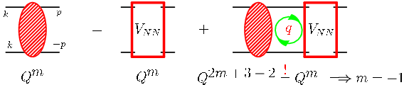
to their non-relativistic mass-shell. Otherwise, one of them could be treated as perturbation of the others and a low-lying bound-state would be absent. Picking the nucleon-pole in the energy-integration leads therefore to the consistency condition that the -scattering amplitude must be of order , irrespective of the potential used. Here, is a typical low-momentum scale of the process under consideration, e.g. the inverse -wave scattering length. The relative strength of forces and potentials in EFT is therefore not just determined by counting the number of momenta. This has long been recognised in “pion-less” EFT, but is only an emerging communal wisdom in the chiral version [19, 18, 17], see also Birse’s contribution to these proceedings.
In deuteron Compton scattering, this mandates to include whenever both nucleons propagate close to their mass-shell between photon absorption and emission, i.e. when the photon energy does not suffice to knock a nucleon far off its mass-shell [19].

Figure 3 lists the contributions to Compton scattering off the deuteron to next-to-leading order NLO in EFT. At higher photon energies , the nucleon is kicked far enough off its mass-shell, , for the amplitude to become perturbative. This is intuitively clear, as the struck nucleon has only a very short time () to scatter with its partner before the second photon has to be radiated to restore the coherent final state. The diagrams which contain in Fig. 3 are therefore less important for larger , together with some of the other diagrams. Indeed, the nucleon propagator becomes static and scales as , with each re-scattering process in suppressed by an additional power of . However, -rescattering practically eliminates even at these high energies the dependence on the potential used to produce the deuteron wave-function and -rescattering matrix. We implemented rescattering by the Green’s function method described in [20, 21, 4, 3]. The calculation is parameter-free after fitting the scalar polarisabilities with the result quoted in eq. (2) [4, 3].
2.3 Deuteron Observables
Besides the unpolarised cross-section of Refs. [4, 8, 3], new techniques allow measuring observables with polarised beams and/or targets. For a linearly polarised beam and unpolarised deuteron, is the differential cross-section for photon polarisation in the scattering plane, and for perpendicular polarisation. The double polarised observables involve a vector-polarised deuteron and a circularly or linearly polarised photon. Often, experiments discuss asymmetries , i.e. cross-section differences divided by their sums, to cancel systematic effects. Figure 4 gives a pictorial representation of the observables considered, in lieu of lengthy formulae.
linpol. , unpol. d:
 ,
, 
circpol. ,
vecpol. d
:

,

linpol. ,
vecpol. d
:

,

Cross-section differences and asymmetries for observables, depending on dipole polarisabilities and kinematic variables (photon energy and scattering angles and ) in the cm and lab frame, and additional constraints like the Baldin sum rule and the forward and backward spin-polarisabilities, provide a cornucopia of information which cannot adequately be conveyed in a short article. We therefore focus only on some prominent examples here and note that in order to aide in planning new experiments, the results for all observables are available as an interactive Mathematica 7.0 notebook from Grießhammer (hgrie@gwu.edu). It produces both tables and plots of energy- and angle-dependences from to MeV of all the asymmetries and cross-section differences, as well as of the total cross-section, in both the cm and lab systems, including their sensitivities to varying the spin-independent and spin-dependent polarisabilities independently.
3 Significance of the and Rescattering on Polarisation Observables
We first analyse the and intermediate rescattering contributions on polarisation observables. Figure 5 compares double-polarisation observables within different schemes. The upper (lower) row shows the parallel (perpendicular) polarisation asymmetry () with circularly polarised photons. The left (right) panels are for MeV ( MeV). As for unpolarised observables [4, 8], the does not contribute appreciably at MeV, but the observable is still ruled by including intermediate rescattering for the correct Thomson limit. In contradistinction, the and intermediate -rescattering are equally significant at MeV.


Like in Refs. [4, 8] for unpolarised observables, we find that both the and intermediate rescattering are necessary ingredients to identify polarisation observables for reliably extracting polarisabilities from zero to MeV. We also checked that dependence on the potential used to produce the deuteron wave-function and -rescattering matrix is irrelevant.
4 Results
We now identify selected polarisation observables which are helpful in extracting in particular spin-polarisabilities. For an unpolarised target, is at MeV (lab) appreciable sensitive only to and , see Fig. 6. At 125 MeV (lab) however, the sensitivity to is large and comparable to that of . Amongst double-polarisation observables at 125 MeV, there is also appreciable sensitivity to the polarisabilities in the linear photon polarisation asymmetry , see Fig. 7. The dependences on , and are again comparable. Finally, the circular photon polarisation asymmetry at 125 MeV, shows large and comparable sensitivity on , and now , but only minor sensitivity on the other spin-polarisabilities.


Thus, it is imperative that the values of the electric and magnetic polarisabilities be better extracted so as not to taint any extraction of the spin polarisabilities. While no observable is sensitive only to one dipole polarisability, closely inspecting (1) reveals configurations in which one (or more) polarisabilities do not contribute for nucleon Compton scattering. In the example of Fig. 9, a photon is scattered on an unpolarised nucleon in the cm frame such that the linear photon polarisation is perpendicular to the scattering plane, cf. [22]. A detector under can therefore not detect photons radiated from the induced magnetic dipole in the nucleon. As demonstrated in the figure, this hold even when the relative motion of the nucleon in the deuteron is taken into account [12]. Similar configurations can be identified for other dipole polarisabilities.
5 Concluding Questions
Our results indicate that some observables of single- and double-polarised deuteron Compton scattering can be used to directly extract some of the so-far nearly un-determined spin-polarisabilities. However, as these are higher-order relative to the electric and magnetic polarisabilities, the former can only be extracted reliably when the scalar polarisabilities are known with better accuracy. With this goal, an experiment at MAXlab is being analysed as we speak, and an experiment at HIS is approved. Concurrently, we are improving the theoretical accuracy by including higher orders in EFT [6]. To find all nucleon spin-polarisabilities, one therefore needs to work through:
- (1)
A set of relatively low-energy experiments, MeV, where the spin-polarisabilities are negligible but the scalar polarisabilities can be determined to high accuracy. This will also reveal differences between the proton and neutron polarisabilities and their constituents.
- (2)
With a better handle on and , a combination of concurrent unpolarised and polarised measurements can be used to extract the spin polarisabilities. Most efficient seems a set of double-polarised experiments at MeV but below the pion-production threshold.
In principle, a multipole-analysis of experiments at different angles suffices in step (2) to over-determine the spin-polarisabilities – if the data has unprecedentedly high accuracy. and can to a good degree be extracted uniquely from and , respectively. However, a larger number of independent data will be necessary to account for the high complexity of these experiments, and for the fact that no clear-cut observables exist for the “mixed” spin-polarisabilities and . In each, the accuracy achievable and the observables and kinematics most suited strongly depend on geometry and acceptance of the experimental setup. We have therefore made our detailed results available as interactive Mathematica 7.0 notebook (email to hgrie@gwu.edu).
In the long run, a multipole-analysis of Compton scattering at fixed energies from double-polarised, high-accuracy experiments provides a new avenue to extract the energy-dependence of the six dipole-polarisabilities per nucleon [2]. A concerted effort of planned and approved experiments at is indeed under way: polarised photons on polarised protons, deuterons and 3He at TUNL/HIS; tagged protons at S-DALINAC; polarised photons on polarised protons at MAMI. The unpolarised experiment on the deuteron at MAXlab over a wide range of energies and angles is being analysed [5]. With at present only 28 (un-polarised) points for the deuteron in a small energy range of MeV and error-bars on the order of , high-quality data allow one to zoom in on the proton-neutron differences and provide first information on the spin-polarisabilities. We re-iterate that a publication elaborating on these findings is forthcoming [12].
Enlightening insight into the electro-magnetic structure of the nucleon has already been gained from combining Compton scattering off nucleons and few-nucleon systems with EFT and the (energy-dependent) dynamical polarisabilities; and a host of activities should add to it in the coming years, so that we understand the response of the nucleon spin constituents to external electro-magnetic fields, as parameterised by its spin-polarisabilities.
Acknowledgements
We acknowledge financial support by the National Science Foundation (CAREER grant PHY-0645498) and US Department of Energy (DE-FG02-95ER-40907).
References
- [1] B. R. Holstein, D. Drechsel, B. Pasquini, M. Vanderhaeghen, Phys. Rev. C61, 034316 (2000); M. Schumacher, Prog. Part. Nucl. Phys. 55, 567 (2005).
- [2] R. P. Hildebrandt, H. W. Grießhammer, T. R. Hemmert, B. Pasquini, Eur.Phys.J. A20 293(2004).
- [3] R. P. Hildebrandt, H. W. Grießhammer, T. R. Hemmert, nucl-th/0512063 (2005).
- [4] R. P. Hildebrandt, Ph. D. Thesis, arXiv.org:nucl-th/0512064.
- [5] L. Myers, priv. comm.
- [6] H. Grießhammer, J. McGovern, D. R. Phillips, D. Shukla, work in progress.
- [7] S. R. Beane, M. Malheiro, J. A. McGovern, D. R. Phillips, U. van Kolck, Phys. Lett B567, 200 (2003). Erratum-ibid: Phys. Lett. B607 320 (2005); S. R. Beane, M. Malheiro, J. A. McGovern, D. R. Phillips, U. van Kolck, Nucl. Phys. A747, 311–361 (2005).
- [8] R. P. Hildebrandt, H. W. Grießhammer, T. R. Hemmert, D. R. Phillips, Nucl. Phys., A748, 573 (2005).
- [9] S. R. Beane, M. Malheiro, D. R. Phillips, U. van Kolck, Nucl. Phys. A656, 367–399 (1999).
- [10] D. Choudhury, D. R. Phillips, Phys. Rev. C71, 044002 (2005).
- [11] D. Choudhury, A. Nogga and D. R. Phillips, Phys. Rev. Lett. 98 232303 (2007); D. Shukla, A. Nogga and D. R. Phillips, Nucl. Phys. A819 98 (2009); D. Choudhury, Ph.D. Thesis, (2006).
- [12] H. Grießhammer and D. Shukla, forthcoming.
- [13] H.W. Grießhammer and T.R. Hemmert, Phys. Rev. C 65, 045207 (2002).
- [14] T. R. Hemmert, B. R. Holstein and J. Kambor, Phys. Rev.D55, 5598 (1997); T. R. Hemmert, B. R. Holstein, J. Kambor and G. Knöchlein, Phys. Rev. D57(9), 5746 (1998).
- [15] D.L. Hornidge et al., Phys. Rev. Lett. 84, 2334 (2000).
- [16] J.L. Friar, Ann. of Phys. 95, 170 (1975); H. Arenhövel, Z. Phys. A297, 129 (1980); M. Weyrauch and H. Arenhövel, Nucl. Phys. A408, 425 (1983).
- [17] H. W. Grießhammer, Nucl. Phys. A760 110 (2007).
- [18] A. Nogga et al., Phys. Rev. C72, 054006 (2005); M.C. Birse, Phys. Rev. C74, 014003 (2006) and 76, 034002 (2007).
- [19] H.W. Grießhammer, forthcoming.
- [20] J.J. Karakowski and G.A. Miller, Phys. Rev. C60, 014001 (1999); J.J. Karakowski, Ph.D. thesis U. of Washington 1999 [nucl-th/9901011].
- [21] M.I. Levchuk and A.I. L’vov, Nucl. Phys. A674, 449 (2000).
- [22] L. C. Maximon, Phys. Rev. C 39 (1989) 347.