The atmospheric charged kaon/pion ratio using seasonal variation methods

When cosmic rays interact in the stratosphere, mesons are produced in the primary hadronic shower. These mesons either interact again and produce lower energy hadronic cascades, or decay into high energy muons which can penetrate to detectors deep underground. The temperature of the stratosphere remains nearly constant, only changing slowly over longer timescales such as seasons (with the exception of the occasional Sudden Stratospheric Warming events observed during wintertime at high latitudes [1]). An increase in temperature of the stratosphere causes a decrease in density, reducing the chance of meson interaction, resulting in a larger fraction decaying to produce muons. This results in a higher muon rate observed deep underground [2, 3, 4, 5, 6]. The effect increases as higher energy muons are sampled, because higher energy mesons with increased lifetimes (due to time dilation) are involved. This effect permits the measurement of the atmospheric charged kaon/pion production ratio. The rate of low energy muons at the surface of the earth is also affected by the temperature because the varying production altitude changes the chances of the muon decaying before reaching earth, but this effect is not relevant for detectors deeper than 50 mwe[3] (meters water equivalent).

The intensity of muons underground is directly related to the production of mesons in the stratosphere by hadronic interactions between cosmic rays and the nuclei of air molecules. It is assumed that meson production falls off exponentially as $e^{-X/\Lambda_{N}}$ where $\Lambda_{N}$ is the absorption mean free path of the cosmic rays and X is the slant depth of atmospheric material traversed. It is also assumed that the mesons retain the same direction as their progenitors, that the cosmic ray sky is isotropic in solid angle at the top of the atmosphere, and ionization is neglected. These assumptions are particularly valid for the large energies of the mesons that produce muons seen in deep underground detectors such as Baksan [7], Super-K [8], IceCube [9] and MINOS far detector (MINOS FD) and near detector (MINOS ND) [10]. In this approximation, $\Lambda_{N}$ is constant. Two meson absorption processes will be considered: further hadronic interactions, $dX/\Lambda_{M}$, where dX is the amount of atmosphere traversed, and $M\rightarrow\mu\nu_{\mu}$ decay. The fractional loss of mesons by decay is given by

where $\rho=$ air density, $\tau_{0}=$ mean M lifetime (at rest) [2], and $p_{r}$ is the meson rest frame momentum. M is either a $\pi$ or K meson (charm and heavier meson production doesn’t become important until $\sim 10^{5}\,\mathrm{TeV}$). For an isothermal, exponentially vanishing atmosphere, the atmospheric scale height H(T) = RT/Mg. The density $\rho$ is then related to X by $\rho=X\cos\theta/H(T)$. The critical energy $\epsilon_{M}$, the energy that separates the atmospheric interaction and decay regimes, is given by

Since most interactions take place in the first few interaction lengths [11], and to first order $H(T)~\approx~H_{0}~=~6.5\,\mathrm{km}$, $\epsilon_{\pi}=0.115\,\mathrm{TeV}$, $\epsilon_{K}=0.850\,\mathrm{TeV}$, the differential meson intensity $\mathcal{M}(E,X,\cos\theta)$ can be written as a function of X [2, 11]:

for relativistic M, where $N_{0}(E)$ is the differential M production spectrum which has the form $E_{M}^{-(\gamma+1)}$, $\Lambda_{N}$ is the nucleon interaction length, and $Z_{NM}$ is the spectrum-weighted inclusive cross section moment. This differential equation is straightforward to solve using an integrating factor and rewriting  [2, 11]:

where $1/\Lambda_{M}^{\prime}\equiv 1/\Lambda_{N}-1/\Lambda_{M}$.

Now that an expression for the production and propagation of mesons through the atmosphere has been found, a function describing the production of muons must be found. Muons are produced from mesons via the two body decay process $M\rightarrow\mu\nu$. The rest frame momentum for this decay is $p_{r}=(1-m_{\mu}^{2}/m_{M}^{2})m_{M}/2$ (since the neutrino has negligible mass). The differential flux per unit cross section is proportional to the differential flux per energy, which can be written

where B is the branching ratio and $P_{L}$ is the momentum of the decaying particle in the lab frame. The muon production spectrum for meson M parents is given by Gaisser [11]:

Inserting Eq. 5 into the muon production spectrum (Eq. 6) gives

where $r_{M}=m_{\mu}^{2}/m_{M}^{2}$. Muons are sampled by detectors at one particular depth, so the production spectrum must be integrated over the whole atmosphere to find the energy spectrum of interest. The relevant energy spectrum is written:

where $\gamma=1.7$ is the muons spectral index [12], the branching ratio $B(K\rightarrow\nu_{\mu}\mu)$ = 0.635, and $B(\pi\rightarrow\nu_{\mu}\mu)\simeq$ = 1. The parameters $A_{\pi,K}$ are constants involving the amount of inclusive meson production in the forward fragmentation region, the masses of the mesons and muons, and the muon spectral index [11]:

The integral of the production spectrum can be written in the form [2]

This is the total number of muons with energy greater than the minimum required to reach an underground detector. The threshold surface energy required for a muon to survive to slant depth $d(\theta,\phi)$ (mwe) increases exponentially as a function of d and parameters a(E) and b(E) [11]. Since a and b depend on energy, an iterative procedure can be used to find the threshold energy [12]:

where the energy-dependent parameters $a=0.00195+1.09\times 10^{-4}\ln(E)$ GeV cm²/g and $b=1.381\times 10^{-6}+3.96\times 10^{-6}\ln(E)$ GeV cm²/g [12], at column depth $d(\theta,\phi)$. The threshold energy at the minimum depth of the detectors considered in Sec. 1 are shown in Table 1. Eq. 10 is approximated [2] as

where 0.635$\cdot A_{K}/A_{\pi}\cdot$r(K/$\pi$) = 0.054 [11], [5] and r(K/$\pi$) is the atmospheric K/$\pi$ ratio.

The temperature changes that occur in the atmosphere are not uniform, instead occurring at multiple levels, and neither muon nor meson production occurs at one particular level (see Figs. 1, 2). The perturbations that variations in temperature cause in muon intensity are small, and as a result properly chosen atmospheric weights can be used to approximate the effective temperature of the atmosphere as a whole, $T_{\mathrm{eff}}$. Define $\eta(X)\equiv(T(X)-T_{\mathrm{eff}})/T_{\mathrm{eff}}$, and $\epsilon_{M}=\epsilon^{0}_{M}(1+\eta)$, where $\epsilon^{0}_{M}$ is the constant value of $\epsilon_{M}$ when $T=T_{\mathrm{eff}}$. This is the temperature that would cause the observed muon intensity if the atmosphere were isothermal. To quantify the temperature effect on intensity, the temperature dependence of Eq. 2 needs to be considered. The meson production term in Eq. 3 (which applies to any charged meson: K, $\pi$, etc) can then be expanded:

The analytic solution to this differential equation is difficult to find since $\eta(X^{\prime})$ is an arbitrary function of X’. A solution to first order in $\eta(X^{\prime})$ can be found by expanding the exponential in a power series, and then following the procedure outlined above, beginning with Eq. 5. This solution can be written as $\mathcal{M}(E,X,\cos\theta)=\mathcal{M}^{0}+\mathcal{M}^{1}$, where $\mathcal{M}^{0}(E,X)$ is the solution where $\epsilon_{M}=\epsilon^{0}_{M}$, which occurs at temperature $T=T_{\mathrm{eff}}$ and $\mathcal{M}^{1}(E,X)$ is given by:

If $E\cos\theta\gg\epsilon^{0}_{M}$, then the integrand is very small and $\eta(X^{\prime})=\eta(X)$. This is the case when interactions dominate, as time dilation effects allow these very high energy mesons to travel great distances before decaying. If $E\cos\theta\ll\epsilon^{0}_{M}$, then the mesons will not travel very far before decaying and the integrand is large only when X’ is near X, and again, $\eta(X^{\prime})$ can be taken out of the integral [2].

Writing the solution of $\mathcal{M}$ where $T=T_{\mathrm{eff}}$ as $\mathcal{M}^{0}$ and letting $\epsilon_{M}=\epsilon^{0}_{M}(1+\eta)$, an expression for the change in muon production induced by temperature variations can be found. Define $\Delta\mathcal{M}\equiv\mathcal{M}-\mathcal{M}^{0}$, then to first order in $\eta$

Using Eq. 7 and Eq. 8, an expression for the change in differential muon intensity can be found:

where

Now, a solution to this integral can be found for $E_{\mu}\gg\epsilon^{0}_{M}(I^{H})$ and for $E_{\mu}\ll\epsilon^{0}_{M}(I^{L})$:

These expressions can be combined in a form that is valid for all energies (Eq. 8):

where

The exact solution for $I^{L}_{M}(E_{\mu})$ has been replaced with an approximation that preserves the physical behavior of the system at low energies. These low energy mesons are relatively insensitive to changes in temperature because they decay before they have a chance to interact. So, this equation describes the expected behavior that mesons at very low energies will decay fairly high in the atmosphere. These mesons will not contribute any muons to an underground detector, because the muons they produce will be below the threshold energy.

There is a slight dip in this distribution as X approaches $\Lambda^{\prime}_{M}$, which results from the approximation made to join the high and low energy solutions for the approximation to Eq. 18. The low energy solution will go to zero when $X=\Lambda^{\prime}_{M}$ and below zero when $E_{\mathrm{th}}\ll\epsilon^{0}_{M}$. The reason for this is that these low energy muons have such little energy that they decay in flight, producing a deficit in muons anticorrelated to positive temperature changes (the “negative temperature coefficient” related in older literature [2, 14, 15]). This effect is not seen by detectors deeper than 50 mwe. The fact that there is a dip and subsequent rise in Fig. 1 for $X>480\,\mathrm{g/cm^{2}}$ does not affect an analysis for a detector deeper than 50 mwe since the weight is integrated over the entire atmosphere in discrete steps of dX and properly normalized, so this atmospheric depth is unimportant for the production of relevant muons.

Remembering that $\eta(X)\equiv(T(X)-T_{\mathrm{eff}})/T_{\mathrm{eff}}$, the relationship between atmospheric temperature fluctuations and intensity variations can be written:

where the temperature coefficient $\alpha(X)$ can be written:

with $W^{M}(X)$ given by:

The approximation to the integral follows from arguments made by Barrett [2]. The derivative of this expression agrees with the integrand in the energy region of interest to within 2%. The weights as a function of X using the threshold energies of the detectors under consideration can be seen in Fig. 1. The fact that the lines are nearly on top of each other shows that the weight of the particular atmospheric depth does not depend very much on the threshold energy. Recalling that M applies equally to K and $\pi$ mesons and that the total muon intensity is the sum of the contribution by K and $\pi$ (Eq. 12), the temperature induced change in muon intensity can be written:

Letting $T_{\mathrm{eff}}$ be defined such that when $T(X)=T_{\mathrm{eff}}$, $\Delta I_{\mu}=0$ gives

Since the temperature is usually measured at discrete levels, the integral is calculated numerically over the atmospheric levels $\Delta X_{n}$:

$W^{\pi,K}_{n}$ is $W^{\pi,K}$ evaluated at $X_{n}$, $1/\Lambda_{\pi,K}^{\prime}\equiv 1/\Lambda_{N}-1/\Lambda_{\pi,K}$, $\Lambda_{N}=120\,\mathrm{g/cm^{2}}$, $\Lambda_{\pi}=160\,\mathrm{g/cm^{2}}$ and $\Lambda_{K}=180\,\mathrm{g/cm^{2}}$ [11].

With this definition of Effective Temperature, an Effective Temperature coefficient, $\alpha_{T}$, can be defined:

where $I^{0}_{\mu}$ is the intensity for a given temperature T. Now that the atmospheric temperature has been parametrized and $\alpha_{T}$ defined, the relationship between atmospheric temperature fluctuations and intensity variations can be written:

Note that the expression to calculate $T_{\mathrm{eff}}$ in the pion scaling limit, ignoring the kaon contribution is the same as the MACRO [3] calculation for effective temperature. This distribution reflects the dominant atmospheric phenomena that produce muons visible to a detector underground. High energy mesons produced at the top of the atmosphere have the greatest influence on the seasonal variation because they are created where the density is lower, so they have the highest probability to decay into muons. High energy mesons that are produced lower in the atmosphere have a greater probability of interacting a second time, and thus greater probability of producing muons that are not seen by an underground detector.

The theoretical prediction of $\alpha_{T}$ for properly weighted atmospheric temperature distribution can be written (Eq. 27):

Barrett [2] shows that for a muon spectrum such as Eq. 8, the theoretical $\alpha_{T}$ can be written:

The prediction for $\alpha_{T}$ can be calculated using the intensity found in Eq. 12 and a little algebra:

where

Note that this can be reduced to MACRO’s previously published expression $\left<\alpha_{T}\right>_{\pi}$ [3], which was only valid for pion induced muons, by setting $A^{1}_{K}=0$ (no kaon contribution). This approximation can be extended to a kaon-only temperature coefficient, $(\alpha_{T})_{K}$ by setting the pion term (first term in parentheses) in Eq. 12. The result is an independent model of the temperature coefficient for each of the meson species:

To compare the experimental $\alpha_{T}$ to the theoretical expectation, a simple numerical integration using a Monte Carlo method was performed. A muon energy and $\cos\theta$ were chosen out of the differential muon intensity (Eq. 12). A random azimuthal angle, $\phi$, was chosen and combined with $\cos\theta$. Column depth was calculated as $d=h/\cos\theta$, where h is the detector depth in mwe for standard rock with flat overburden. The threshold surface energy required for a muon to survive this column depth is found from the expression for threshold energy (Eq. 11). If the chosen $E_{\mu}$ was greater than $E_{\mathrm{th}}$, it was used in the calculation of the theoretical $\left<\alpha_{T}\right>$. This was repeated for 10,000 successful muons with $E_{\mu}>E_{\mathrm{th}}$, at depths from 0 to 4,000 mwe.

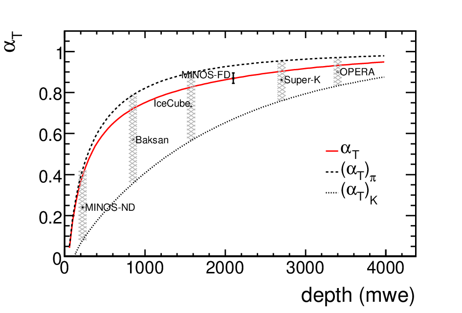
The result of this calculation, along with the experimental result from the MINOS experiment [5] can be seen in Fig. 3 as the solid line. This curve includes the “negative temperature effect” (muon decay correction) term, $\delta^{\prime}=(1/E\cos\theta)(m_{\mu}c^{2}H/c\tau_{\mu})(\gamma/\gamma+1)\ln(1030/\Lambda_{N}\cos\theta)$ [2], which goes to zero for $E_{\mu}>50\,\mathrm{GeV}$.

The kaon component of air showers that can be observed at 1400 mwe is about 10%, but the energy is too low for kaon-induced muon production to be affected by changes in temperature. The result is the large gap between the pion only curve and the K$\pi$ curve. As the depth increases, the energy of sampled muons also increases, which results in a greater contribution to $\alpha_{T}$ by kaon induced muons. The asymptotic behavior of the theoretical $\alpha_{T}$ approaching one as primary energy increases is expected from Eq.28. At very high primary energies, the intensity is proportional to the critical meson energy, which depends on temperature. Thus, for an isothermal atmosphere, intensity will be directly proportional to the temperature (the constant of proportionality, $\alpha_{T}$, will be one).

The theoretical uncertainty of the atmospheric K/$\pi$ ratio is of order 40 % [16]. There was not a measurement of this ratio with cosmic rays until 2009, when it was made using MINOS FD data [5]. Previous measurements have been made at accelerators for p+p collisions [17], Au+Au collisions [18], Pb+Pb collisions [19, 20].

The expression for the experimental $\alpha_{T}$ is written in Eq. 27. The kaon influence causes an overall decrease in total $\alpha_{T}$, shown in Sec. 4. Because the left hand side of Eq. 27 depends only on counting rate, it can be broken into meson components:

which can be rewritten:

Recall that in the pion scaling limit, only pions are assumed to contribute to the seasonal effect. From that, a model for pion-only and kaon-only temperature coefficients were developed in Eq. 32. Such a seasonal effect can be written:

The ratio of the muon counting rates $R^{K}_{\mu}/R^{\pi}_{\mu}$ is equivalent to the ratio of muons from kaons to muons from pions $N^{K}_{\mu}/N^{\pi}_{\mu}$, which will be written $r_{\mu}(K/\pi)$. Rearranging and inserting Eq. 35 for both kaons and pions into Eq. 33 gives:

The value for $r_{\mu}(K/\pi)$ can be predicted by integrating Eq. 12:

where

The parameter $A^{1}_{K}$ is defined as

where $r(K/\pi)=\frac{Z_{NK}}{Z_{N\pi}}$ [11] is the ratio of kaons to pions produced in the primary cosmic ray interactions. Inserting Eq. 41 into Eq. 38 and rearranging gives an expression for $r(K/\pi)$ in terms of $r_{\mu}(K/\pi)$:

The MINOS-FD [5] measurement is shown in Fig. 4, along with STARS [18], NA49 [19, 20] and ISR [17] accelerator measurements. The cross-hatched regions show the energy regimes to which the underground detectors discussed in this paper are sensitive for $K/\pi$ ratio measurements using the method described.

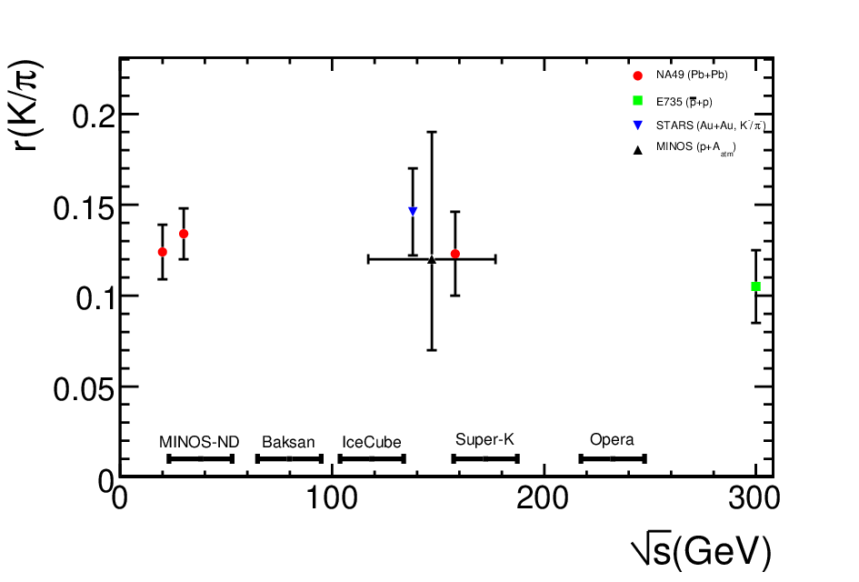
An OPERA measurement would extend to the region an order of magnitude beyond the energy of current fixed target experiments. With a detector area roughly 1,000 times the area of the MINOS FD, IceCube should have a cosmic ray muon rate of upon completion of construction (Boreal Spring, 2011) of 1,700 Hz [21]. Assuming a temperature data set of comparable quality to the BADC ECMWF data [22] used by the MINOS-FD analysis [5], the statistical uncertainty in $\alpha_{T}$ could be reduced to $\pm 0.001$. Since the absorber material surrounding IceCube is ice instead of rock containing iron veins, the column depth should be more well known. This could reduce the uncertainty in the depth map, the dominant source of uncertainty in $(\alpha_{T})_{\pi,K}$, by half. These factors taken together could reduce the uncertainty in the measurement of $r(K/\pi)$ by 16-30%.

A new method was developed to include the effect of kaons in measurement of seasonal variations in underground muon intensity. A temperature coefficient that accounts for the kaon contribution was described, and a kaon-inclusive model was defined. These methods were applied to MINOS-FD data [5], and the new model fit the data better than the pion only model [3]. A formula was described so that other underground experiments, OPERA, Super-K, IceCube, Baksan and the MINOS ND could quickly apply this method to their data. Pion and kaon decay are affected differently by temperature variations, and this difference suggested a method to measure the atmospheric K/$\pi$ ratio. This method was developed and a formula was offered for other underground experiments to follow.

We thank our many colleagues who provided vital input as these methods were developed, especially Tom Kelley for providing comments on the presentation of the mathematics. This work was supported by the U.S. Department of Energy, the U.K. Science and Technologies Facilities Council, the U.S. National Science Foundation, the Center for Cosmology and AstroParticle Physics at Ohio State University and the University of Minnesota. We also acknowledge the BADC and the ECMWF for providing the environmental data for this project.

References

- [1] S. Osprey, et al., Sudden stratospheric warmings seen in MINOS deep underground muon data, Geophys. Res. Lett. 36 (2009) L05809.
- [2] P. Barrett, et al., Interpretation of cosmic-ray measurements far underground, Rev. Mod. Phys. 24 (1952) 133–175.
- [3] M. Ambrosio, et al., Seasonal variations in the underground muon intensity as seen by MACRO, Astropart. Phys. 7 (1997) 109–124.
- [4] A. Bouchta, Seasonal variation of the muon flux seen by AMANDA, Proc. 26th Int. Cosmic Ray Conf., Salt Lake City 2 (1999) 108.
- [5] P. Adamson, et al., Observation of muon intensity variations by season with the MINOS far detector, Submitted to Phys. Rev. D, hep-ex/09094012.
- [6] S. Tilav, et al., Atmospheric variations as observed by IceCube, Proc. 31st Int. Cosmic Ray Conf., Lodz.
- [7] E. N. Alexeyev, et al., Proc. 16th Int. Cosmic Ray Conf., Kyoto 10 (1979) 276.
- [8] Y. Fukuda, et al., The Super-Kamiokande detector, Nucl. Instrum. Meth. A501 (2003) 418–462.
- [9] J. Ahrens, et al., IceCube: The next generation neutrino telescope at the South Pole, Nucl. Phys. Proc. Suppl. 118 (2003) 388–395.
- [10] D. G. Michael, et al., The magnetized steel and scintillator calorimeters of the MINOS experiment, Nucl. Instrum. Methods 596 (2008) 190–228.
- [11] T. K. Gaisser, Cosmic rays and particle physics, Cambridge, UK: Univ. Pr. (1990) 279 p.
- [12] P. Adamson, et al., Measurement of the atmospheric muon charge ratio at TeV energies with MINOS, Phys. Rev. D76 (2007) 052003.
- [13] J. K. De Jong, Measurement of the atmospheric muon charge ratio using the MINOS near detector, Proc. 30th Int. Cosmic Ray Conf., Merida.
- [14] G. Cini Castagnoli, M. Dodero, II Nuovo Cim. B 51 (1967) 525.
- [15] J. Humble, et al., Proc. 16th Int. Cosmic Ray Conf., Kyoto 4 (1979) 258.
- [16] G. D. Barr, T. K. Gaisser, S. Robbins, T. Stanev, Uncertainties in atmospheric neutrino fluxes, Phys. Rev. D74 (2006) 094009.
- [17] A. M. Rossi, et al., Experimental Study of the Energy Dependence in Proton Proton Inclusive Reactions, Nucl. Phys. B84 (1975) 269.
- [18] C. Adler, et al., Kaon production and kaon to pion ratio in Au + Au collisions at = 130-GeV, Phys. Lett. B595 (2004) 143–150.
- [19] S. V. Afanasiev, et al., Energy dependence of pion and kaon production in central Pb + Pb collisions, Phys. Rev. C66 (2002) 054902.
- [20] C. Alt, et al., Inclusive production of charged pions in p p collisions at 158-GeV/c beam momentum, Eur. Phys. J. C45 (2006) 343–381.
- [21] J. Ahrens, et al., Status of the IceCube Neutrino Observatory, New Astron. Rev. 48 (2004) 519–525.
- [22] European Centre for Medium-Range Weather Forecasts ECMWF Operational Analysis data, [Internet] British Atmospheric Data Centre 2006-2007, Available from http://badc.nerc.ac.uk/data/ecmwf-op/.