Looping of the numbers game and the alcoved hypercube
Abstract.
We study in detail the so-called looping case of Mozes’s game of numbers, which concerns the (finite) orbits in the reflection representation of affine Weyl groups situated on the boundary of the Tits cone. We give a simple proof that all configurations in the orbit are obtainable from each other by playing the numbers game, and give a strategy for going from one configuration to another. The strategy gives rise to a partition of the finite Weyl group into finitely many graded posets, one for each extending vertex of the associated extended Dynkin diagram. These are selfdual and mutually isomorphic, and dual to the triangulation of the unit hypercube by reflecting hyperplanes, studied by many authors. Unlike the weak and Bruhat orders, the top degree is cubic in the number of vertices of the graph. We explicitly compute the Hilbert polynomial of the poset.
1. Introduction
1.1. The numbers game
Mozes’s game of numbers [Moz90], which originated from (and generalizes) a 1986 IMO problem, has been widely studied (cf. [Pro84, Pro99, DE08, Eri92, Eri93, Eri94a, Eri94b, Eri95, Eri96, Wil03a, Wil03b]), and yields useful algorithms for computing with the root systems and reflection representations of Coxeter groups (see [BB05, §4.3] for a brief summary).
We briefly recall the numbers game. Consider a Coxeter group associated to generators , and relations , for ( for all , and for ). We associate to this an unoriented graph with no loops and no multiple edges, with vertex set , such that two vertices are adjacent if . Consider also a choice of Cartan matrix such that for all , whenever and are not adjacent, and in the case are adjacent, and either (when is finite), or (when ).
The configurations of the game consist of vectors , considered as labelings of the graph by numbers called amplitudes. The moves of the game are as follows: for any vector and any vertex such that , one may perform the following move, called firing the vertex : is replaced by the new configuration , defined by
| (1.1) |
The entries of the vector are called amplitudes. The game terminates if all the amplitudes are nonnegative. Let us emphasize that only negative-amplitude vertices may be fired.
Note that the operation is nothing but the action of the simple reflection if is in the basis of the fundamental coweights (or weights).
The following summarizes some basic known results (where denotes the usual dot product in , and in the case of affine Coxeter groups, denotes a generator of the kernel of the Cartan form, in the basis of simple roots; the precise definition is recalled in §2):
Theorem 1.2.
- (i)
- (ii)
In the finite Coxeter group case, the numbers game must terminate.
- (iii)
[Eri94a] In the affine case, the numbers game terminates if and only if .
- (iv)
[Eri94a] Whenever the numbers game does not terminate, it reaches infinitely many distinct configurations, except for the affine Coxeter group case where , in which case only finitely many configurations are reached (i.e., the game “loops”).
In particular, we will be concerned here with the looping case.
We explain briefly how our results relate to standard constructions in the theory of Coxeter groups. The configuration space is the reflection representation of the Coxeter group . The subset of where the numbers game terminates is called the Tits cone. The Tits cone is naturally divided into simplicial cones, with the maximal cones labeled by the elements of (see [BB05, Sections 4.3 and 4.9]). Beginning with a point in the interior of one of these maximal cones, the cones we travel through form a descending chain in the weak order (whose definition we recall in §4.2); the restriction of firing only negative amplitudes means that we only move downward. So results (i) and (ii), in part, say that weak order is graded and has a unique minimal element.
Our results study the affine case, not within the Tits cone, but at its boundary. In the affine case, the boundary of the Tits cone is a hyperplane, divided into finitely many simplicial cones. The maximal cones are indexed by the elements of a finite Coxeter group, . However, our problems do not reduce to the numbers game on , but instead reveal several new and interesting combinatorial structures.
1.2. Motivation and results
The original motivation of this paper was the following question: in the affine case with , can one always return to the initial configuration? This was asserted to be true in [Eri94a],11 1 Also, there it was asserted that there is a way to play the numbers game that passes through all configurations in the Weyl orbit of the vector exactly once (i.e., that a Hamiltonian cycle exists in the directed graph whose vertices are this Weyl orbit and directed edges are moves of the numbers game). We do not have either a proof or counterexample to this assertion. but a proof was not provided. Our first goal is to provide a simple proof in the affirmative. In fact, we prove more: we give in §3 a strategy for going from any configuration to any element of its Weyl orbit in a number of moves cubic in the number of vertices, and our strategy is optimal in certain cases.
In the process, we find (in §4) that, following our strategy, the graph of obtainable configurations leads to a canonical decomposition of the finite Weyl group associated to our graph into graded selfdual posets, one for each extending vertex, whose maximal degree is cubic in the number of vertices (unlike the weak order poset, which has quadratic degree in the number of vertices). The vertices are a canonical choice of coset representatives modulo the subgroup which acts by automorphisms on the extended Dynkin graph. Moreover, we show that the graph of this poset coincides with the dual of the triangulation of the unit hypercube in the reflection representation of the affine Weyl group. This triangulation has been studied in many places, notably recently in [LP07] in type .
Finally, in §5, we compute the Hilbert polynomial of this poset, thus significantly strengthening our initial result, and give explicit formulas. Going from the lowest to top degree element of the poset involves a canonical involution of the extended Dynkin graph which we also compute. In §5.2, we give a combinatorial interpretation and proof of this formula in the type cases.
Evaluating the Hilbert polynomial at in two ways yields a curious identity (which was unknown to us): Let be a finite Weyl group associated to a Dynkin graph with vertex set , and let be the corresponding affine Weyl group and extended Dynkin graph, with . Let be the Coxeter exponents of . Then,
| (1.3) |
where the elements are those that take the dominant chamber of (i.e., the locus where all coordinates are nonnegative) to its translate by , for is the -th fundamental coweight (which is the -th basis vector of our configuration space ), and is the length of , i.e., the minimum number of simple reflections whose product is .
1.3. Acknowledgements
We thank T. Lam for essential discussions about the Hilbert polynomials of our posets. The first author is an EPDI fellow, the second author is an AIM fellow, and the third author is a Clay research fellow. The first two authors were supported by Clay Liftoff fellowships. The second author was also partially supported by the University of Chicago’s VIGRE grant. We thank the University of Chicago, MIT, and the Isaac Newton Institute for Mathematical Sciences for hospitality.
2. Preliminaries on affine Coxeter groups
In this note, we will be concerned with the numbers game when is an extended Dynkin graph, and is the standard integral matrix associated to it (we can generalize this to the case where is nonintegral but satisfies whenever is odd: see Remark 3.9). In the simply-laced case (types , or ), this just means that all the entries of are or . In all other types, where is a simply-laced graph, is a (nontrivial) subgroup of , and the matrix is obtained from the matrix as above by the usual folding procedure, i.e., for and adjacent, is equal to the number of elements of which fix divided by the number which fix both and .
The interesting phenomena already occur in the simply-laced case, and the reader can assume this to be the case if preferred.
We will make use of the root systems associated to Dynkin and extended Dynkin graphs. Let be the set of roots and positive roots, respectively. We will view in the basis of simple roots. Then, the dot product between roots and configuration vectors (viewed as coweights) is the canonical pairing.
To be precise, by roots we mean what are sometimes called real roots, i.e., the images of the simple roots under the Coxeter group action dual to the action: , where is the -th simple root and is the Cartan form, .
For an extended Dynkin graph , a vertex is called extending if the complement of the graph is a Dynkin graph with respect to which the given vertex is the extending vertex. Finally, we will make use of the element , uniquely given so that at all extending vertices of the graph, and for all .
We emphasize that is the set of roots for the affine Coxeter group. On the occasion that we need to refer to the root system of the associated finite Coxeter group, we write ; then will denote the set of positive roots from .
3. Strong looping of the numbers game
In this section, we prove and generalize the following:
Theorem 3.1.
Whenever the numbers game loops, one can always return to the initial configuration.
Recall that the numbers game loops if and only if the Coxeter group is affine and the initial configuration satisfies . The theorem can be re-expressed as: if , then for every element of the Coxeter group of the graph, one can go from to by playing the numbers game.
As in the introduction, let be integral and given by an identification where is simply-laced. Playing the numbers game on is equivalent to playing on the -invariant configurations on . Making this choice of does not affect the validity of the theorem.
We will prove a stronger result, which gives a strategy for obtaining from whenever and are in the same (affine) Weyl orbit, and a bound on the number of moves required (which will be cubic in the number of vertices of ).
To explain this, first note that, whenever , is uniquely determined by its restriction to any subgraph obtained by removing exactly one vertex. We now fix a subgraph such that is the extending graph of (i.e., corresponds to a finite Coxeter group, and corresponds to the associated affine Coxeter group). Let be the finite Coxeter group associated to . For any configuration on , let denote the restriction to . Similarly, for any configuration on , let be the unique configuration on such that and . Then, for any configuration on such that , and any element , the configuration makes sense. Moreover, any sequence of moves of the numbers game can be represented as applying an element of , since firing the extending vertex is the same (when ) as applying the reflection about the maximal root of .
Thus, we can reformulate the theorem as follows: for any two Weyl chambers of , and every vector , there exists a way to play the numbers game on to take to a vector whose restriction to is in .
Next, note that one can always play the numbers game on until all the amplitudes on are nonnegative: this yields the unique configuration obtainable from the original one which is in the dominant Weyl chamber. Similarly, by playing the numbers game in reverse, one sees that every configuration is obtainable from one in the antidominant Weyl chamber. Thus, to prove the theorem, it is enough to show that one can take every vector of the dominant Weyl chamber to a vector of the antidominant Weyl chamber. Moreover, for this it suffices to take any single vector in the interior of the dominant Weyl chamber: we will take the vector , where is the vector on whose amplitude is at all vertices.22 2 corresponds to one-half the sum of all positive coroots of (or the sum of all fundamental coweights), and is important in Lie theory.
Let be the vertex set of and be the vertex set of the fixed subgraph . Let be the extending vertex of . Set . For any other extending vertex (i.e., such that the extended Dynkin graph of is ), let also denote the configuration with such that for all (i.e., is the image of under an automorphism of ). We may now strengthen Theorem 3.1:
Theorem 3.2.
For any , beginning with and playing the numbers game by arbitrarily firing vertices of amplitude , one obtains for some extending vertex . Regardless which moves are chosen, the total number of moves is the same, as is the vertex . Moreover, this is the fastest way, under the numbers game, to get from to a configuration of the form . Finally, taking , the resulting map is an involution on the extending vertices of .
Moreover, the score vector is the same regardless of the moves chosen: this means the configuration vector on which records, at each vertex of , the sum of negative all the amplitudes fired in the course of playing the game.
To prove the theorem, we will use two lemmas:
Lemma 3.3.
Let have the following properties:
- (i)
is in the boundary of the Tits cone, i.e., .
- (ii)
For each , .
- (iii)
For every root , .
Then for some extending vertex .
Note in particular that, for any , the vector satisfies (i) and (iii).
Proof.
Recall that denotes the root system of . The simple roots of are the simple roots for , together with , where is the longest root in . Using (i) and (ii), we deduce that for in .
Taking inner product with yields a linear function on , which, by condition (iii), is not zero on any root. Let be the subset of whose inner product with is negative; so for some . For any , for some nonnegative integers , and then . If is an element of which is not of the form then we deduce that , and thus .
Combining the observations of the last two paragraphs, we see that . Suppose, for the sake of contradiction, that for some . Then lies in the closed half-space whose boundary is spanned by the simple roots other than . But there is a positive linear dependence between the elements of , which is a contradiction.
We deduce that . So is for all but one element . Viewing as an element of , this says that all but one coordinate is . Let that one coordinate be . Consider the simple roots of associated to ; modulo , these roots form a simple root system for (namely, ). So, is an extending vertex and . ∎
Lemma 3.4.
Beginning with any configuration , suppose that is possible to fire vertices (counted with multiplicity) of amplitude until there are none left. Consider any other sequence of firing vertices of amplitude . Then and this sequence can be extended to a sequence of firings of vertices of amplitude which terminates at the same configuration.
Corollary 3.5.
Beginning with any configuration , suppose there are two ways of firing vertices of amplitude until there are none left. Then these two paths are of the same length, and terminate at the same configuration.
Proof of Lemma 3.4.
This is very similar to the proof of strong convergence in the numbers game, so we will be brief. Our proof is by induction on . Notice that, if and then the coordinate will still be after the -vertex is fired. Thus, if then only one coordinate of is and the claim is obvious.
For larger , let be our sequence of length , beginning by firing , and let be the sequence of length , beginning by firing . Then and are both . Consider alternately firing and until both coordinates are . (If this never occurs, then no path from can terminate.) Let be the configuration when both coordinates become . We claim that this configuration does not depend on whether we fire or first and the two paths and have the same length . In fact, if is even, and if is odd. It is clear that applying firings, alternating between firing vertex and , produces the desired result, regardless of which reflection is applied first: we only have to prove that, along the way, only vertices of amplitude are fired. This follows because, by usual strong convergence of the numbers game, only negative-amplitude vertices are fired; these amplitudes must be of the form where is a positive root for the restriction of the diagram to vertices and . Therefore, is a vector with nonpositive integral entries, implying that the dot product is indeed .
By induction, we can extend to a path of length . Tacking the second part of this path onto the path , we obtain a path of length . Using induction again, we can complete to a path . Tacking on the beginning of this path, we are done. ∎
Note that there is nothing in the above lemma that requires the number : the same is true for any negative number, and neither the number nor need be integral.
Proof of Theorem 3.2.
We begin by showing that there is a path from any to some by firing only vertices of amplitude . Start at and fire vertices of amplitude in any manner. Since the orbit of is finite, either we will reach a configuration with no vertices of amplitude , or we will repeat a configuration. In the former case, by Lemma 3.3, we are done. In the latter case, we have a path of the form . Reversing this path and negating all the configurations, we obtain a path which only fires vertices of amplitude . So we have two paths of different lengths from to , contradicting Lemma 3.4. Note that we now have enough to prove Theorem 3.1.
We continue with the proof of Theorem 3.2. Let be of the form . Because the numbers game for terminates, it is possible to get from to by firing only vertices of negative amplitude. By the result we just established, it is possible to get from to some by firing only vertices of negative amplitude. Let the length of a shortest path from to some be ; we must show that this path involves only firing vertices of amplitude . Our proof is by induction on ; the base case is obvious. If is of the form , we are clearly done. If not then, by Lemma 3.3, for some .
Let the first step of our path go from , firing . The rest of the path, from to , must be a shortest path from to any and hence, by induction, must only involve firing vertices of amplitude . Let . We want to show that .
Starting at , alternately fire and until the and coordinates are both positive. The resulting configuration, , is the same whether we fire or first, and the length of the resulting path from to is in either case. On the route from to , all the vertices fired are of amplitude . Using Lemma 3.4, we can fire more vertices of amplitude to get from to . Now, consider the path which starts by firing . Then the vertex which is fired when going from to has amplitude . The path from to must be shortest possible (or there is a shorter path from to ). So, by induction, every vertex which is fired in this path has amplitude . In particular, and the original path fires only vertices of amplitude .
It remains only to show that, for , the resulting map on extending vertices of is an involution. For this, note that if a firing sequence of vertices of amplitude takes to , then the sequence in reverse takes to , also by vertices of amplitude . ∎
Remark 3.6.
One may easily compute the involution appearing above:
Proposition 3.7.
The involution is trivial for exactly the graphs
| (3.8) |
For graphs , is the involution sending every vertex in to its antipodal vertex. For type , interchanges exterior vertices which are adjacent to a common internal vertex, and is the identity on interior vertices. For types , is the unique nontrivial automorphism of the graph.
We will explain the proof following Lemma 4.3 in the next section.
Remark 3.9.
The results of this section generalize to the case when the Cartan matrix is not necessarily integral, but satisfies whenever is odd. This is because, in this case, every positive root is obtained from a simple root by simple reflections that only increase coordinates in the basis of simple roots. Hence, for every positive root and every configuration such that , we must have , with equality holding only if is a simple root such that . Then, all of the statements of results above remain unchanged, except that, in Lemma 3.3, we should let be in the Weyl orbit of a vector such that for all , leaving the conditions (i)–(iii) unchanged. The proofs are only changed to replace the integrality by the above fact.
Note that the results do not hold in general without the assumption that for odd : for instance, a counterexample to Lemma 3.4 is obtained if we consider the Dynkin graph with Cartan matrix and the vector , then one firing sequence yields , firing only vertices of amplitude , whereas the other firing sequence yields , and then we would have to fire a vertex of amplitude to obtain the same configuration as in the previous firing sequence. As a result, the configuration on the diagram with Cartan matrix contradicts Theorem 3.2. Moreover, the vector contradicts Lemma 3.3, as generalized in the previous paragraph.
4. The resulting poset and geometric interpretations
In this section, in Proposition 4.1, we relate playing the numbers game on the boundary of the Tits cone, where we fire only vertices of amplitude beginning from , with playing the numbers game slightly inside the Tits cone where we fire any vertex with negative amplitudes beginning with configurations of the form , for appropriate values of . Recall that is the -th fundamental coweight, which is also the -th basis vector of configuration space .
We then study the posets of configurations obtainable from by firing vertices of amplitude , and see how these give rise to a canonical decomposition of the finite Weyl group into isomorphic graded selfdual posets, , one for each extending vertex, whose maximal degree is cubic in the number of vertices (unlike the weak order poset, which has quadratic degree in the number of vertices). Then, using Proposition 4.1, we show how the poset may be identified with an interval under the left weak order in the affine Weyl group.
Finally, we also show that the graph of this poset coincides with the dual of the triangulation of the unit hypercube in the reflection representation of the affine Weyl group. This triangulation has been studied in many places, notably recently in [LP07] in type .
4.1. Relation to strong convergence, and number of moves required
Here, we compare firing only amplitudes beginning from with firing any negative amplitudes beginning from the configuration , for certain positive values of . Using this, strong convergence of the numbers game for will explain why can reach and why the strategy of (arbitrarily) firing vertices of amplitude is the fastest way to do so. This will also allow us to easily compute the number of moves required.
Let be the longest root of .
Proposition 4.1.
If , then a sequence of vertices is a valid firing sequence for the numbers game beginning with if and only if it is a firing sequence of amplitudes beginning with . Moreover, the final configurations reached under a maximal such sequence are and , respectively, for some fixed involution .
The proposition relies on the following basic, and probably well known, lemma (whose proof we supply for the reader’s convenience). For each vertex , let be the “translation” element of the form
| (4.2) |
Let be the coweight lattice (with basis the fundamental coweights ) and let be the coroot sublattice. In the basis of fundamental coweights, , where for all .
Lemma 4.3.
For any vertex , there is a unique element whose action on is of the form , where is a permutation of coordinates corresponding to an automorphism of the graph . Moreover, the map induces a group monomorphism .33 3 The group is well known and called the fundamental group of the root system.
Proof.
Fix and let us consider the hyperplane , fixed under . It suffices to show that the lemma holds restricted to . Note that the triangulation of by its intersection with the Weyl chambers has the translational symmetry . Thus, there must exist a unique element such that takes the dominant Weyl chamber (i.e., the one whose amplitudes are all nonnegative) to its translate under . We must therefore have that is an isometry of the dominant Weyl chamber. Thus, is induced by an automorphism of .
To see that this induces a homomorphism , we need to show that the all commute with each other. When is not of type or , this is immediate since is abelian. In the case of type , an easy computation shows that, when is adjacent to , then is a rotation of the diagram (moving each vertex to an adjacent one), and it is easy to see that all the can be obtained from products of conjugates of this one, and therefore that the images of the generate the abelian normal subgroup , in this case. In the case of type , the image of is a -element subgroup of and is hence abelian (we can also compute explicitly that the image is abelian, like in type ).
Finally, we need to show that the kernel of is . Let denote the reflection corresponding to the maximal root , so . Let us define
| (4.4) |
Then, is a translation if and only if , and in this case,
can be written as a product of conjugates of the translation . In other words, the translations of are exactly . ∎
We remark that the above lemma also allows one to prove Proposition 3.7, using the statement of Proposition 4.1. Indeed, for as in Proposition 4.1, we see that is in the same affine Weyl orbit as (since, by playing the numbers game on the Dynkin subgraph , one may go from to ). Thus, is in the affine Weyl orbit as the final configuration , which is in the Weyl chamber containing , and hence is obtainable from by applying translates . Thus, the formula for follows by computing the automorphisms , which is not difficult (and probably well known).
Proof of Proposition 4.1.
When we play the numbers game beginning with , let us keep track of not only the resulting configuration , but also the vector , where is replaced by an indeterminate , and such that valid firing sequences beginning with are, by definition, sequences that become valid when is evaluated at .
First, we claim that, playing the numbers game in this way from , any amplitude of the form that appears must have . The reason for this is that, if , then , and since this is negative, it can only appear by playing the numbers game if for some positive root , but the latter is impossible. Therefore, when playing the numbers game beginning with , we never fire an amplitude of the form , for . As a consequence, any firing sequence for which becomes valid when is evaluated at , must also be a firing sequence for where only amplitudes are fired.
Next, we claim that, if , then the numbers game beginning with terminates at the configuration , and that playing the same moves from yields . By Lemma 4.3, the element is in the -orbit of , for some automorphism . If we evaluate at we get a dominant weight (in fact all coefficients are positive, so we get a regular dominant weight), and thus the numbers game can only terminate at , and since , the numbers game must terminate.
As a consequence of the previous two paragraphs, for any , and any maximal valid firing sequence beginning at , the same firing sequence takes to . (Note that this gives another proof of Theorem 3.1.)
It remains to show that any firing sequence from of amplitudes is also a valid firing sequence for with as above. Let be the number of moves of any firing sequence as above. By Theorem 3.2, any maximal firing sequence of vertices of amplitude takes to , in exactly the same number of moves, .
Therefore, any firing sequence of length beginning with of vertices of amplitude must take to a configuration which can win the numbers game (arrive at ) in moves. As a result, the sequence must be a valid firing sequence for , since each move must have decreased by one the set of positive roots which pair negatively with the current configuration. ∎
In the case that , we may immediately deduce a formula for the number of moves required to go from to . Indeed, this equals the number of positive roots such that when . For any positive root such that , then , where is any positive root supported on a segment containing , of length . Let us identify , with , and with two integers adjacent if they differ by one modulo . Then, to pick a pair of and the integer is equivalent to picking the triple of distinct integers in . Thus, the total number of such is .
As a result, to go from any configuration with to , it takes no more than moves. Indeed, assume without loss of generality that . Then, letting be the extending vertex such that can be obtained from by firing vertices of amplitude , it can take at most moves to go from to , and and then at most moves to go from there to .
We will prove a more general result (and for any extended Dynkin graph) in §5 below.
4.2. The poset obtained from the strategy
For each extending vertex , let be the poset of configurations obtainable from by firing vertices of amplitude . By Theorem 3.2,
| (4.5) |
Moreover, each is a graded poset: this means that each element has a well-defined degree, given by the number of firings of vertices with amplitude needed to go from to . They are also self-dual, which means that the poset is isomorphic to the one where the ordering is reversed.
It is clear that the are all isomorphic posets. Since acts freely on , we may view (4.5) as a decomposition of itself into isomorphic graded posets, . Moreover, the isomorphism is nothing but , where is the element such that .
We remark that (4.5) is quite canonical. In particular, it does not depend on the choice of the dominant vector : any element whose restriction to is in the interior of the dominant Weyl chamber (i.e., all amplitudes are positive) gives rise to the same decomposition (4.5), except that are now defined as the graded posets of configurations obtainable along a minimal-length firing sequence from to . When we pass to the decomposition of itself into isomorphic graded posets, the result is independent of .
As we saw at the end of the previous section, is quite different from the weak or Bruhat orders on : rather than having at most quadratic degree in the number of vertices of the Dynkin diagram, we have cubic degree. The elements of the poset are a canonical choice of representatives of the right cosets of the group generated by the (which is a subset of ).
As a consequence of Proposition 4.1, the poset may be identified with an interval under the (left) weak order in the affine Weyl group—we explain this below. First, note that, for any element obtained from by a sequence of firings of amplitudes , Proposition 4.1 shows that the element depends only on and not on the choice of firing sequence. That is, we obtain an embedding . Let be the resulting composition. This is a section of the quotient defined by for any (that is, for , and is the reflection about the maximal root of ). Precisely, is the inclusion. We will now show that the image poset is nothing but an interval in under the weak order.
We recall the definition of weak order. For , the length of , denoted , is the minimal number of simple reflections needed to multiply to . The left weak order in is the ordering such that if and only if , and the right weak order in is the ordering such that if and only if .
Generally, define the numbers game ordering to be: is less than if can be obtained from by playing the numbers game.
Lemma 4.6.
Let be any graph associated to a Coxeter group . Given any configuration for which the numbers game terminates at for , then the map restricts to an isomorphism of the interval with the numbers game poset from to .
Proof.
By strong convergence, if a valid firing takes to , where , is dominant, then . As a consequence, it inductively follows that it takes exactly moves to take to by playing the numbers game. The result follows immediately. ∎
Returning to our situation, let be the top degree element, i.e., . We immediately deduce
Corollary 4.7.
The isomorphism takes the poset to the interval .
4.3. Triangulation of the unit hypercube in the reflection representation
Denote by the “unit hypercube” in the hyperplane . Note that is a fundamental domain under the group generated by the translations used in Lemma 4.3, and its image under is the hypercube .
Let us associate to the poset the directed graph whose vertices are elements of and whose directed edges are such that is obtained from by firing a single vertex of amplitude (i.e., ).
Let be the dominant Weyl chamber, i.e., . To any polytope that is the union of Weyl chambers, we associate a dual directed graph, which is the usual dual graph forgetting orientation, with orientation given by when .
Proposition 4.8.
The graph is isomorphic to the dual of the triangulation of the unit hypercube by Weyl chambers.
Proof.
The dual of the triangulation of is the interval under the right weak order, where is the longest element such that . We claim that . Given the claim, the result follows immediately from the fact that is isomorphic to under the inversion map (which sends the left weak order to the right weak order).
To prove the claim, first note that the Weyl chamber containing is in and is the one incident to the corner of that is opposite to , i.e., to the corner given by for . (To see that and are in the same Weyl chamber, one can take very close to without changing which chamber is in, which would make very close to .) Next, observe that, by Proposition 4.1, the element is in the dominant Weyl chamber . Thus, is the longest element which takes to , i.e., we must have . ∎
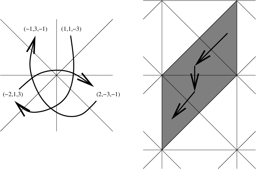
In figure 1, we demonstrate the above concepts in type . On the left, we depict the graph . The point means the point of with those coordinates. Our convention is that the first coordinate corresponds to the root of , the second coordinate to the root of , and the third coordinate to , the negation of the longest root. On the right, we show the unit hypercube of , and how occurs as the dual to this hypercube.
5. The Hilbert polynomial of
In what follows, we will consider any subset of as being endowed with the graded poset structure given by the right weak order, . Also, for any finite Coxeter group associated to a graph with vertex set , let be its Coxeter exponents.
Recall that the Hilbert polynomial of a graded poset is defined as
| (5.1) |
where denotes the degree of . We may explicitly compute the Hilbert polynomial of the graded poset :
Theorem 5.2.
The Hilbert polynomial of is given by
| (5.3) |
Here, the elements are the translations as defined in the Lemma 4.3.
Note that, evaluating the polynomial at and using that decomposes into isomorphic copies of , one copy for each extending vertex, we obtain (1.3).
We remark that there is always a way to rearrange the factors in the denominator, i.e., to assign to each vertex an exponent , so that is a polynomial. In some sense, this can be done uniquely: see §5.1.
Proof.
Let be the semigroup generated by the elements defined in Lemma 4.3, i.e., the elements of the form , where , the ’s were defined in 4.2, and . We claim that
| (5.4) |
where is the subgroup generated by the reflections for , and moreover that every element has a unique decomposition as where , , and , satisfying
| (5.5) |
As a consequence, by taking Hilbert series (using the well known formulas [BB05, Theorems 7.1.5, 7.1.10] for and ),
| (5.6) |
which proves the theorem, subject to proving (5.4), (5.5), which we do now. Applying both sides to the fundamental Weyl chamber in , the statement is saying that a fundamental domain for in is given by the image of the dominant Weyl chamber under , i.e., the cone . This follows from the fact that, under the projection by forgetting the -coordinate, this cone is the preimage of the dominant -chamber in . ∎
5.1. Explicit formulas for
Below we give each Dynkin graph , with vertices labeled by two positive integers: , and a Coxeter exponent such that , so that each occurs once. We will need the following notation: the odd part, , of is the maximal odd factor of .
Set . Then, by Theorem 5.2,
| (5.7) |
which is a factorization of by polynomials whose nonzero coefficients are all .
The top degrees of the posets are the degrees of the Hilbert polynomials, given from the figure by:
.
For the series of types and , these degrees are cubic in the number of vertices; in the exceptional cases, one may find similar identities, such as , and ). An upper bound on the number of valid moves in the numbers game required to go from any vector on the extended Dynkin graph satisfying to any element of its Weyl orbit is given by the sum of this degree and the weak order degree of (the latter being quadratic in the number of vertices), and is therefore cubic in the number of vertices.
Let us consider the question of how unique the assignment of the exponents to the vertices is such that . For exceptional types, this assignment of the exponents to the vertices is unique, except in the case, where it is unique up to swapping with when are images of each other under an element of . For each infinite series, one can make a uniqueness statement if one views the collection of graphs for all together. For example, for types , and , if we label the vertices for such a series subject to the condition that the maximal segment of consecutively-numbered vertices goes to infinity, then this is the unique assignment of so that the are given by a polynomial in and or the odd part of such a polynomial. For type , this is true except for the first vertex which is assigned a different polynomial, .
We remark that, for types and , even though their finite Weyl groups are identical, Hilbert polynomials , and in particular . However, ; indeed, both must equal . Moreover, .
5.2. Combinatorial interpretation of the Hilbert polynomial for type
In this section, we consider the case of . In the proof of Theorem 5.2, we computed the Hilbert series of the inverse image in of the dominant Weyl chamber for ; specifically, we showed that this series is . In [EE98, Section 9.4], Eriksson and Eriksson gave a combinatorial proof of this result. We sketch their proof, and explain how to modify it to give a combinatorial proof of Theorem 5.2. Let here and be the affine and finite Weyl groups of types and , respectively.
Let be the set of permutations of the integers such that and . Define a map by ; it is well known that this map is injective and its image is . So, we can identify with . Under this identification, the dominant chamber consists of those permutations with . The unit hypercube consists of those permutations where, in addition, , , …, and .
Given in the dominant chamber, define an -tuple as follows: Let be an integer between and . Let be the set of integers such that and , , …, . Number the elements of as . So, is in ; define by .
Remark 5.8.
The integer is the number of times that occurs in the sequence constructed in [EE98].
It is easy to see that this is a bijection between the dominant chamber and . It is also clear that the unit hypercube corresponds to the set .
Proposition 5.9.
Let be in the dominant chamber. Under this bijection, the length of is .
Proof.
We claim that if and only if . Proof: There are precisely elements of which are greater than . Now, is greater than ; if and only if , , …, are all greater than ; if and only if , , …, are the largest elements of ; if and only if .
We prove the proposition by induction on . The result is obvious when all of the are zero, so we may assume this is not true. Let and . So . Consider the element , in the dominant chamber, where . It is not hard to verify that the new vector is . Let denote ; conjugation by is a length preserving automorphism of . Then, , where is an cycle and the right hand side is length-additive, so . ∎
So we have a bijection between the unit hypercube and where the element corresponding to has length . This gives a bijective proof that the Hilbert series of the unit hypercube is .
We note that Eriksson and Eriksson also give combinatorial proofs of the Hilbert series for other classical types; these proofs might be able to be similarly adapted.
References
- [BB05] A. Björner and F. Brenti, Combinatorics of Coxeter groups, Springer, New York, 2005.
- [DE08] R. G. Donnelly and K. Eriksson, The numbers game and Dynkin diagram classification results, arXiv:0810.5371, 2008.
- [EE98] H. Eriksson and K. Eriksson, Affine Weyl groups as infinite permutations, Electronic J. Combin. (1998).
- [Eri92] K. Eriksson, Convergence of Mozes’s game of numbers, Linear Algebra Appl. 166 (1992), 151–165.
- [Eri93] by same author, Strongly convergent games and Coxeter groups, Ph.D. thesis, KTH, Stockholm, 1993.
- [Eri94a] K. Eriksson, Node firing games on graphs, Jerusalem combinatorics ’93: an international conference in combinatorics (May 9–17, 1993, Jerusalem, Israel), vol. 178, Amer. Math. Soc., 1994, pp. 117–128.
- [Eri94b] K. Eriksson, Reachability is decidable in the numbers game, Theoret. Comput. Sci. 131 (1994), 431–439.
- [Eri95] by same author, The numbers game and Coxeter groups, Discrete Math. 139 (1995), 155–166.
- [Eri96] K. Eriksson, Strong convergence and a game of numbers, European J. Combin. 17 (1996), no. 4, 379–390.
- [LP07] T. Lam and A. Postnikov, Alcoved polytopes I, Discrete Comput. Geom. 38 (2007), 453–478, math/0501246.
- [Moz90] S. Mozes, Reflection processes on graphs and Weyl groups, J. Combin. Theory Ser. A 53 (1990), no. 1, 128–142.
- [Pro84] R. A. Proctor, Bruhat lattices, plane partition generating functions, and minuscule representations, European J. Combin. 5 (1984), 331–350.
- [Pro99] by same author, Minuscule elements of Weyl groups, the numbers game, and -complete posets, J. Algebra 213 (1999), 272–303.
- [Wil03a] N. J. Wildberger, A combinatorial construction for simply-laced Lie algebras, Adv. in Appl. Math. 30 (2003), 385–396.
- [Wil03b] by same author, Minuscule posets from neighbourly graph sequences, European J. Combin. 24 (2003), 741–757.