Entropy Perturbations in N-flation
Abstract
In this paper we study the entropy perturbations in N-flation by using the formalism. We calculate the entropy corrections to the power spectrum of the overall curvature perturbation . We obtain an analytic form of the transfer coefficient , which describes the correlation between the curvature and entropy perturbations, and investigate its behavior numerically. It turns out that the entropy perturbations cannot be neglected in N-flation, because the amplitude of entropy components is approximately in the same order as the adiabatic one at the end of inflation . The spectral index is calculated and it becomes smaller after the entropy modes are taken into account, i.e., the spectrum becomes redder, compared to the pure adiabatic case. Finally we study the modified consistency relation of N-flation, and find that the tensor-to-scalar ratio () is greatly suppressed by the entropy modes, compared to the pure adiabatic one () at the end of inflation.
pacs
98.80.CqI Introduction
Inflation is now a standard paradigm for describing the physics of the very early universe, but the microphysics nature of the field(s) responsible for inflation remains unknown. In the last few decades intensive effort has been devoted to understanding the fundamental physics of the inflation theory. For simplicity, most of studies have been focused on the effective single scalar field model, however, in the low-energy limit of string theory, more than one scalar fields are present and they may work cooperatively to drive the inflation, such as the assisted inflation [1].
Recently, Dimopoulos et al. [2] showed that the many axion fields predicted by string vacua can be combined and lead to a radiatively stable inflation, called N-flation. Using the random matrix theory Easther and McAllister [3] showed that the mass distribution for axion fields should be in the Marcěnko-Pastur spectrum form. Further, many cosmological observable imprints of N-flation have been investigated, such as the tensor-to-scalar ratio [4], the non-Gaussianity parameter [5, 13], and the scalar spectral index [6] for the pure adiabatic perturbation. The results show that for and the deviations from the single-field models are negligible, however, the spectral index is smaller than the case of the single-field models. The preheating process after N-flation is numerically investigated in [7] and the results show that the parametric resonance is suppressed which differs significantly from the single-field case.
Compared with the single field model, the presence of multiple fields during inflation can lead to quite different inflationary dynamics [8] (see [9] for a review). In particular, multiple fields can lead to the generation of entropy (non-adiabatic) perturbations during inflation, which can alter the evolution of the overall curvature perturbation [10] and produce a detectable non-Gaussianity [11]. For a two-field model the entropy perturbations are investigated both analytically and numerically [12], however, the generalization from the two-field model to the model with a large number of fields is less developed. For the N-flation model the entropy perturbations have been investigated by different approaches [13, 14]. By virtue of the formalism [15], an analytic form of spectral index is derived in [13], and similar result is obtained by the authors of [14] by using a different approach [16]. In this paper, using the new interpretations of the formalism which are developed in [17], we calculate the entropy corrections to the power spectrum of the overall curvature perturbation, corresponding spectral index and the tensor-to-scalar ratio. Our numerical results are in agreement with the earlier results in [13, 14].
This paper is organized as follows. In Sec. II we briefly review the constructions of N-flation and the mass distribution of axion fields, then investigate the cosmological background evolutions numerically. In Sec. III we study the linear perturbation, derive explicitly the entropy corrections to the primordial power spectrum, and then calculate the power spectrum, spectral index and the tensor-to-scalar ratio numerically for the N-flation model. Sec. IV is devoted to our conclusions.
II Review of N-flation
In this section we briefly review the construction of N-flation, especially focus on the quadratic potential and the mass spectrum. Then we investigate the cosmological background dynamics with a given mass distribution.
II.1 Quadratic potential in N-flation
Dimpopoulos in [2] consider a potential of axions as
| (1) |
where is the periodic potential which arises solely from non-perturbative effects, is the axion decay constant and is the dynamically generated scale of the axion potential that typically arises from an instanton expansion. This scale can be many orders of magnitude smaller than the Planck scale.
For small field values the periodic potentials can be Taylor expanded as
| (2) |
with the masses . Consider the case in which the masses are distributed uniformly and the axion fields start out displaced from the minimum by , with the maximum displacement set by each axion decay constant
| (3) |
then it is effectively equivalent to the scenario of a single field with a super-Planckian displacement . This means that the typical initial condition in the large limit is expected to be super-Planckian and it is suitable for chaotic inflation. In this sense, N-flation realizes the inflation in a very well-controlled string theory setting.
The authors of [2] assume a uniform axion mass spectrum for simplicity, however, for a realistic model we should exactly determine which sorts of mass spectra are possible in string compactification. Surprisingly, in the limit, using the random matrix theory Easther and McAllister [3] obtained an essentially universal mass spectrum, without invoking details of the compactification, such as the intersection numbers, the choice of fluxes, or the location in moduli space.
II.2 Mass spectrum
Consider the Lagrangian of axions with kinetic and potential terms as
| (4) |
where the supergravity potential and the KKLT superpotential reads [18]
| (5) | |||||
| (6) |
with run over the dilaton , the complex structure moduli , and the Kähler moduli . Inserting (6) into (5), expanding the potential around the origin , and using the F-flatness conditions , we have
| (7) |
where the mass matrix is 11 1 Here we emphasize that the moduli , , which appear in , are not dynamical variables.
| (8) |
From (4) and (8), it is easy to see that the kinetic terms and the mass matrix are obviously not diagonal in the basis where the superpotential is simple. We now perform two orthogonal rotations to diagonalize and . First, we rotate the basis to make the axion kinetic terms be canonical
| (9) |
where the mass matrix becomes
| (10) |
We perform the second orthogonal rotation so that is diagonalized, because the potential simply takes a purely quadratic form. In order to reach a more clear result, it is helpful to introduce a new rectangular matrix
| (11) |
then the mass matrix becomes
| (12) |
Because we do not know about the individual terms , in what follows we will regard them as random variables, i.e., we take as a random matrix. Now the task is to determine the eigenvalue spectra of the random matrix. Surprisingly, with the random matrix theory, authors of [3] find that in the large limit the mass spectrum is independent of concrete values of and then obtain an essentially universal mass spectrum
| (13) |
for , where is the ratio of the dimensions of the rectangular matrix , is the variance of the entries of and , are defined as
| (14) | |||||
| (15) |
The spectrum (13) is nothing, but the Marcěnko-Pastur (MP) spectrum. The normalized MP spectrum (13) describes the mass distribution probability of a single axion field. On the other hand, the law of large numbers ensures that the mass distribution of axion fields obeys the distribution probability of the single field. In practice we uniformly split the mass range of axions into () bins
| (16) |
where and the width of each bin are
| (17) |

Furthermore we set the masses of the axions in each bin as
| (18) |
Due to the law of large numbers we then have the following relation
| (19) |
where denotes the number of axions in the th bin.
Note that the constraint from the renormalization of Newton’s constant requires , i.e., [2], in this paper we therefore focus on the model with . By introducing a convenient dimensionless mass parameter and corresponding mass spectrum , we show in Fig. 1 the mass distribution of axion fields in the case of . The parameters and are defined as
| (20) | |||
| (21) |
with .
II.3 Background dynamics
In the previous subsection we have obtained the mass spectrum for the axion fields by virtue of the random matrix theory. Now we discuss the cosmological background dynamics with the MP spectrum. In a flat Friedmann-Robertson-Walker universe, the background dynamics is described by the set of equations
| (22) | |||||
| (23) | |||||
| (24) |
where we have taken the units with . In the slow roll region
| (25) |
one has the scaling solution as
| (26) |
where denotes the initial time of inflation.
In the large limit, we can deal with the masse distribution of axions by employing the MP spectrum. Consequently, the summation over in the equations (22) and (23) becomes integrals over mass as
| (27) | |||||
| (28) |
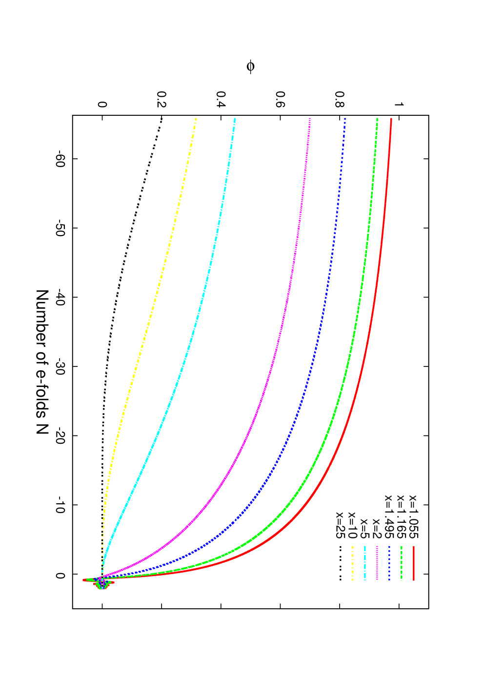
In principle one can solve the evolution equations (24), (27) and (28) for one of the fields, such as the lightest field, then use the scaling solution (26) to get the solutions for other fields during the slow roll period. Because of the complication of the MP spectrum , however, it is very difficult to perform the integration analytically. In this paper we solve the set of background equations (22) and (24) numerically (see Fig. 2), in which we consider axion fields evolving from the equal-energy initial configurations with the vacuum expectation value (vev) of the lightest field, , at the initial time . Our results show that at the initial stage of inflation, only the heaviest fields (such as ) begin rolling down the potential, after a Hubble time, the heaviest fields are no longer over-damped. Instead of immediately becoming under-damped and oscillating they remain critically damped due to the existence of the lighter fields, and the potential energy of the heavier fields is dissipated away before it is converted into kinetic energy. As a result, inflation is mainly sustained by the lighter fields at the late time and ends till the lightest field is no longer over-damped.
III Linear perturbations
In this section using the formalism, we investigate the entropy perturbations during inflation at the linear perturbation level. In the linear cosmological perturbation theory the scalar perturbations of spacetime are usually parameterized as
| (29) |
where is the scale factor, , , and are four scalar perturbations. One can define two important gauge invariant quantities as
| (30) |
In the following subsections we first review the formalism and then analyze the entropy perturbations during inflation by using the method proposed by Tye, Xu and Zhang in [17], and finally calculate the power spectrum, spectral index and the tensor-to-scalar ratio numerically.
III.1 Brief review of the formalism
The primordial curvature perturbation on large scales can be usually calculated by use of the formalism [15]. (For a multi-field inflation model the formalism is nicely reviewed in [17].) One of the essential assumptions of the formalism is the “separate universe assumption” [19], in which separate Hubble volume evolves like separate Friedmann-Robertson-Walker universe where density and pressure may take different values, but are locally homogeneous. Due to the different e-folding numbers between separate Hubble patches, the large scale curvature perturbation on the uniform energy density slice can be expressed as the e-folding number difference between the uniform energy density slice and the unperturbed spatially flat slice at the end of inflation
| (31) |
where and are the number of e-folds on the uniform energy density slice and spatially flat slice respectively. denotes the field configurations at the time of horizon crossing and stands for the time at the end of inflation. In general, can be expanded, up to the second order perturbations, as
| (32) |
where the expansion coefficients are defined as , and is the perturbation of (30) in the spatially flat gauge.
In the multi-field scenario, it turns out convenient to identify the effective inflaton field as the path length of the trajectory in the dimensional field space
| (33) |
where the vector is defined by
| (34) |
Furthermore, one introduces other entropy basis vectors to form a set of orthogonal basis , where and denotes the entropy fields in shorthand. Then the evolution equations for the background fields (24) can be written as the evolution equation for the effective single field
| (35) |
where the potential gradient in the direction is
| (36) |
Thus the unperturbed e-folding number in the direction can be expressed as22 2 One can prove that the e-folding number in (37) is equivalent to the usual definition as long as the potential takes the decoupled form and all fields roll monotonically during inflation. We thank Jiajun Xu for useful correspondence about this point.
| (37) |
and at the linear order, reads
| (38) | |||||
where denotes the field perturbations in entropy directions . As pointed out in [17], the first term above comes from the shift in the initial value , and it corresponds to the adiabatic perturbation in the single field case. The second term arises when the uniform energy slice at the end of inflation is not orthogonal to the background trajectory. And the third and fourth terms are both dependent on the complete inflation trajectory after , which reflects the fact that under the entropy perturbations, the inflaton follows a new trajectory with different length (the third term) and also different speed (the fourth term).
For simplicity, in this paper we ignore the contributions from the second term and rewrite the last two terms using some geometric tricks33 3 The detailed derivations can be found in the Appendix A of [17]., then (38) becomes
| (39) |
with
| (40) |
One can see from (39) that, although there exist entropy modes, can only the one which is along the direction seed the curvature perturbation. Therefore we can use the two-field formalism [12] to discuss the entropy perturbation.
III.2 Observational predictions
Now we calculate the observational predictions of N-flation, such as the scalar power spectra , spectral index and the tensor-to-scalar ratio . In order to calculate the power spectrum of the curvature perturbation, it is convenient to move to the momentum space. The Fourier mode of reads
| (41) |
Using the formalism and choosing the standard Bunch-Davies vacuum,
| (42) |
the two-point correlation functions of the curvature perturbation can be expressed as
| (43) | |||||
where the quantities with subscript denote the quantities take the values at horizon crossing and the slow roll parameters are defined by
| (44) |
With the help of the orthogonal relation among the entropy basis vectors
| (45) |
the second term of the right hand side of (43) can be expressed as
| (46) |
with
| (47) |

For a two-field model one can argue on a very general ground that the time dependence of curvature and entropy perturbations in the large-scale limit can always be described by [12]
| (48) |
where 44 4 In this paper, is denoted as and the sound speed because the kinetic term is canonical in the N-flation model.
| (49) |
and , are two time dependent dimensionless functions. Integrating (48), one can obtain a general form of the transfer matrix which relates the curvature and entropy perturbations generated at horizon crossing to those at some later time
| (50) |
where
| (51) |
As we have shown in (39), for the multi-field model, can only one entropy mode, which is along the direction, contribute to the overall curvature perturbation if we neglect the torsion in the background trajectory. That is to say, we can take as the entropy perturbation in the direction, namely, at the linear perturbation level the multi-field model is effectively equivalent to the two-field model. The relation (50) is still valid in the N-flation model.
With the above results, the power spectrum of the primordial curvature perturbation can be expressed as
| (52) |
where the transfer coefficient
| (53) |
measures the contribution to the overall curvature perturbation from the entropy modes. The first constant term in (52) comes from the pure adiabatic perturbation at the horizon crossing, and the second term, which is time dependent, describes the entropy contributions to the curvature perturbation. Because of the existence of the entropy modes, the curvature perturbation does not conserve after the horizon crossing, and the second term does characterize the time evolution of the spectrum from the horizon crossing to the end of inflation. In Fig. 3, we show the time evolutions of the power spectra with different wavelengthes numerically. The results show that the amplitudes of spectra decrease with the increasing of the perturbation wavenumber , which implies a red tilt spectrum.
In order to further confirm the above analysis about the power spectrum, we calculate the spectral index explicitly. The spectral index turns out to be
| (54) | |||||
where we have fixed and the reads
| (55) | |||||

We plot in Fig. 4 the scalar index versus the logarithm of dimensionless comoving wavenumber . It can be seen from the figure that compared to the pure adiabatic case, the index becomes smaller after including the entropy components. This numerical results are in agreement with the analytic ones in [13, 14].
Finally we discuss the modified consistency relation [9, 20] in N-flation. Because the tensor perturbation is decoupled from the scalar one at the linear order, the gravitational wave power spectrum is frozen-in on large scales as what happens in the single-field model
| (56) |
We define the tensor-to-scalar ratio for a given mode which crosses horizon at e-folding number as
| (57) | |||||
where we have introduced a dimensionless correlation angle
| (58) |
We can see from (57) that, after taking into account the entropy perturbations, the tensor-to-scalar ratio () is always smaller than the one for the case of the pure adiabatic perturbation (). In Fig. 5 we show the tensor-to-scalar ratio of the mode which crosses horizon at e-folding number . The results show that the ratio () is greatly suppressed by the entropy modes at the end of inflation.

IV Conclusion
In this paper we studied numerically the dynamics of N-flation. At the background evolution level we investigated the evolution of axions with the Marcěnko-Pastur mass distribution, and we found that at the initial stage of inflation, only the heaviest fields begin sliding down the potential, after a Hubble time the heaviest fields are no longer over-damped. Instead of immediately becoming under-damped and oscillating they remain critically damped due to the existence of the lighter fields, and all the potential energy of the heavier fields is dissipated away before it is converted into the kinetic energy. As a result the inflation is mainly sustained by the lighter fields at the late time and ends until the lightest field were no longer over-damped.
At the linear perturbation level, we calculated the corrections of entropy perturbations to the power spectrum of the overall curvature perturbation by use of the formalism. We obtained an analytic form of the transfer coefficient , which describes the correlation between the curvature and entropy perturbations, and investigated its behavior numerically. Our results show that the entropy perturbations cannot be neglected in the N-flation model, because the amplitude of entropy components is approximately in the same order as the adiabatic one at the end of inflation . Then we calculated the spectral index and found that the index becomes smaller once the entropy modes are included, i.e., the spectrum becomes redder than the pure adiabatic one. Finally we studied the modified consistency relation for the N-flation model and found that the tensor-to-scalar ratio () is greatly suppressed by the entropy modes, compared to the pure adiabatic one () at the end of inflation.
In this paper we only considered the entropy perturbations from the third and fourth terms in the right hand side of (38), which depend on the whole background trajectory in field space, while ignored the corrections to the curvature perturbation which would arise when the uniform energy slice at the end of inflation was not orthogonal to the background trajectory. In addition, the additional power in the curvature perturbation, which may be produced by the (p)reheating process, is also out of the discussion in this paper.
Acknowledgements.
BH thanks Seoktae Koh for useful discussions and Jiajun Xu for helpful correspondence. BH and RGC are supported in part by the National Natural Science Foundation of China under Grant Nos. 10535060, 10821504 and 10975168, and by the Ministry of Science and Technology of China under Grant No. 2010CB833004. YSP is supported in part by NSFC under Grant No: 10775180 and by the Scientific Research Fund of GUCAS,References
- [1] A. R. Liddle, A. Mazumdar and F. E. Schunck, “Assisted inflation,” Phys. Rev. D 58, 061301 (1998) [arXiv:astro-ph/9804177]. N. Kaloper and A. R. Liddle, “Dynamics and perturbations in assisted chaotic inflation,” Phys. Rev. D 61, 123513 (2000) [arXiv:hep-ph/9910499]. P. Kanti and K. A. Olive, “Assisted chaotic inflation in higher dimensional theories,” Phys. Lett. B 464, 192 (1999) [arXiv:hep-ph/9906331]. Y. S. Piao, R. G. Cai, X. m. Zhang and Y. Z. Zhang, “Assisted tachyonic inflation,” Phys. Rev. D 66 (2002) 121301 [arXiv:hep-ph/0207143].
- [2] S. Dimopoulos, S. Kachru, J. McGreevy and J. G. Wacker, “N-flation,” JCAP 0808, 003 (2008) [arXiv:hep-th/0507205].
- [3] R. Easther and L. McAllister, “Random matrices and the spectrum of N-flation,” JCAP 0605, 018 (2006) [arXiv:hep-th/0512102].
- [4] L. Alabidi and D. H. Lyth, “Inflation models and observation,” JCAP 0605, 016 (2006) [arXiv:astro-ph/0510441].
- [5] D. Battefeld and T. Battefeld, “Non-Gaussianities in N-flation,” JCAP 0705, 012 (2007) [arXiv:hep-th/0703012]. S. A. Kim and A. R. Liddle, “Nflation: Non-gaussianity in the horizon-crossing approximation,” Phys. Rev. D 74, 063522 (2006) [arXiv:astro-ph/0608186].
- [6] S. A. Kim and A. R. Liddle, “Nflation: Multi-field inflationary dynamics and perturbations,” Phys. Rev. D 74, 023513 (2006) [arXiv:astro-ph/0605604]. Y. S. Piao, “On perturbation spectra of N-flation,” Phys. Rev. D 74, 047302 (2006) [arXiv:gr-qc/0606034]. S. A. Kim and A. R. Liddle, “Nflation: observable predictions from the random matrix mass spectrum,” Phys. Rev. D 76, 063515 (2007) [arXiv:0707.1982 [astro-ph]]. J. O. Gong, “End of multi-field inflation and the perturbation spectrum,” Phys. Rev. D 75, 043502 (2007) [arXiv:hep-th/0611293].
- [7] D. Battefeld and S. Kawai, “Preheating after N-flation,” Phys. Rev. D 77, 123507 (2008) [arXiv:0803.0321 [astro-ph]].
- [8] A. J. Christopherson and K. A. Malik, “The non-adiabatic pressure in general scalar field systems,” Phys. Lett. B 675, 159 (2009) [arXiv:0809.3518 [astro-ph]]. D. Langlois, “Cosmological perturbations from multi-field inflation,” J. Phys. Conf. Ser. 140, 012004 (2008) [arXiv:0809.2540 [astro-ph]]. D. Langlois and S. Renaux-Petel, “Perturbations in generalized multi-field inflation,” JCAP 0804, 017 (2008) [arXiv:0801.1085 [hep-th]].
- [9] D. Wands, “Multiple field inflation,” Lect. Notes Phys. 738, 275 (2008) [arXiv:astro-ph/0702187].
- [10] C. Gordon, D. Wands, B. A. Bassett and R. Maartens, “Adiabatic and entropy perturbations from inflation,” Phys. Rev. D 63, 023506 (2001) [arXiv:astro-ph/0009131].
- [11] X. Gao and B. Hu, “Primordial Trispectrum from Entropy Perturbations in Multifield DBI Model,” JCAP 0908, 012 (2009) [arXiv:0903.1920 [astro-ph.CO]].
- [12] J. Garcia-Bellido and D. Wands, “Metric perturbations in two-field inflation,” Phys. Rev. D 53, 5437 (1996) [arXiv:astro-ph/9511029]. D. Wands, N. Bartolo, S. Matarrese and A. Riotto, “An observational test of two-field inflation,” Phys. Rev. D 66, 043520 (2002) [arXiv:astro-ph/0205253]. D. Langlois, “Correlated adiabatic and isocurvature perturbations from double inflation,” Phys. Rev. D 59, 123512 (1999) [arXiv:astro-ph/9906080].
- [13] T. Battefeld and R. Easther, “Non-gaussianities in multi-field inflation,” JCAP 0703, 020 (2007) [arXiv:astro-ph/0610296].
- [14] K. Y. Choi, J. O. Gong and D. Jeong, “Evolution of the curvature perturbation during and after multi-field inflation,” JCAP 0902, 032 (2009) [arXiv:0810.2299 [hep-ph]].
- [15] A. A. Starobinsky, “Multicomponent de Sitter (Inflationary) Stages and the Generation of Perturbations,” JETP Lett. 42, 152 (1985) [Pisma Zh. Eksp. Teor. Fiz. 42, 124 (1985)]. M. Sasaki and E. D. Stewart, “A General Analytic Formula For The Spectral Index Of The Density Perturbations Produced During Inflation,” Prog. Theor. Phys. 95, 71 (1996) [arXiv:astro-ph/9507001]. D. H. Lyth, K. A. Malik and M. Sasaki, “A general proof of the conservation of the curvature perturbation,” JCAP 0505, 004 (2005) [arXiv:astro-ph/0411220]. M. Sasaki and T. Tanaka, “Super-horizon scale dynamics of multi-scalar inflation,” Prog. Theor. Phys. 99, 763 (1998) [arXiv:gr-qc/9801017].
- [16] D. Polarski and A. A. Starobinsky, “Isocurvature perturbations in multiple inflationary models,” Phys. Rev. D 50, 6123 (1994) [arXiv:astro-ph/9404061].
- [17] S. H. Tye, J. Xu and Y. Zhang, “Multi-field Inflation with a Random Potential,” JCAP 0904, 018 (2009) [arXiv:0812.1944 [hep-th]].
- [18] S. Kachru, R. Kallosh, A. Linde and S. P. Trivedi, “De Sitter vacua in string theory,” Phys. Rev. D 68, 046005 (2003) [arXiv:hep-th/0301240].
- [19] D. Wands, K. A. Malik, D. H. Lyth and A. R. Liddle, “A new approach to the evolution of cosmological perturbations on large scales,” Phys. Rev. D 62, 043527 (2000) [arXiv:astro-ph/0003278]. D. H. Lyth and D. Wands, “Conserved cosmological perturbations,” Phys. Rev. D 68, 103515 (2003) [arXiv:astro-ph/0306498].
- [20] N. Bartolo, S. Matarrese and A. Riotto, “Adiabatic and isocurvature perturbations from inflation: Power spectra and consistency relations,” Phys. Rev. D 64, 123504 (2001) [arXiv:astro-ph/0107502].