Constraints on primordial isocurvature perturbations and spatial curvature
by Bayesian model selection
Abstract
We present posterior likelihoods and Bayesian model selection analysis for generalized cosmological models where the primordial perturbations include correlated adiabatic and cold dark matter isocurvature components. We perform nested sampling with flat and, for the first time, curved spatial geometries of the Universe, using data from the cosmic microwave background (CMB) anisotropies, the Union supernovae (SN) sample and a combined measurement of the integrated Sachs–Wolfe (ISW) effect. The CMB alone favors a (positively correlated) isocurvature contribution in both the flat and curved cases. The non-adiabatic contribution to the observed CMB temperature variance is at 98% CL in the curved case. In the flat case, combining the CMB with SN data artificially biases the result towards the pure adiabatic CDM concordance model, whereas in the curved case the favored level of non-adiabaticity stays at 3% level with all combinations of data. However, the ratio of Bayes factors, or , is more than 5 points in favor of the flat adiabatic CDM model, which suggests that the inclusion of the 5 extra parameters of the curved isocurvature model is not supported by the current data. The results are very sensitive to the second and third acoustic peak regions in the CMB temperature angular power: therefore a careful calibration of these data will be required before drawing decisive conclusions on the nature of primordial perturbations. Finally, we point out that the odds for the flat non-adiabatic model are 1:3 compared to the curved adiabatic model. This may suggest that it is not much less motivated to extend the concordance model with 4 isocurvature degrees of freedom than it is to study the spatially curved adiabatic model, though at the moment the model selection disfavors both of these models.
pacs
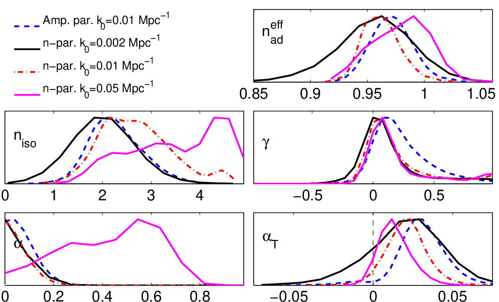
98.80.Es, 98.80.CqI Introduction
Observations of the cosmic microwave background (CMB) [1] and distant supernovae (SN) [2] have shaped the Lambda cold dark matter (CDM) standard model of Cosmology. However, being based on phenomenology, this model still needs better understanding of some of its phases, in particular the origin of the perturbations and the recent-time accelerated expansion of the Universe.
The paradigm of cosmic inflation is often assumed to describe the early history of the Universe; however, many different inflationary theories exist [3] that are still compatible with current data from the CMB and the large scale structure (LSS) of the Universe, and it is therefore interesting to look for ways to distinguish between them.
The primordial perturbations are usually believed to have formed from quantum fluctuations in the early Universe, stretched by inflation. There are two possible types of perturbations that can be thus generated: single-field inflation can only produce adiabatic (isentropic) modes of curvature perturbation , while multi–field models can also generate isocurvature (entropy) perturbations [4]. In Ref. [5] four classes of isocurvature perturbations were identified: the cold dark matter (CDM), baryon, neutrino density, and neutrino velocity isocurvature modes. A generic perturbation can be composed as a linear combination of these ones and an adiabatic mode. However, it has turned out difficult to find physical mechanisms to stimulate for example the neutrino velocity isocurvature mode. In this paper we study a correlated mixture of adiabatic and CDM isocurvature modes (later called the mixed model), that is naturally generated in multi–field inflationary models and in curvaton(-like) models [6, 7, 8, 9, 10]. Other scenarios that may generate observationally compatible isocurvature include axions [11, 12], dilaton [13] and ekpyrotic [14, 15] models, brane inflation [16, 17], large scale magnetic fields [18, 19], cosmic strings and other topological defects [20, 21], whereas an isocurvature mode in interacting dark energy models may grow catastrophically [22, 23, 24].
Physically the inclusion of a CDM isocurvature mode is well motivated. It simply means that initially, at a time , deep in the radiation dominated era on super-Hubble scales, the relative number densities of CDM and photons are not spatially constant, and therefore the total entropy perturbation does not vanish everywhere. In addition to the amplitude (or indeed the variance) of and at , other important observables of the primordial perturbations are the tilt of their power spectrum, parameterized by the spectral index , and their (non-)Gaussianity.
At later times and lower energies, the CMB is an almost perfectly isotropic radiation that has been generated at the epoch of hydrogen recombination. At even more recent times, some additional effects can alter the CMB, such as the integrated Sachs-Wolfe (ISW) effect [25], which is originated by the decay of the gravitational potentials. The most recent and complete ISW data have been obtained by [26] combining data from the CMB and six galaxy catalogs.
It is remarkable that the initial conditions of the CMB are set by the final conditions of inflation. For this reason, we can distinguish between different models of the early universe if we can show which initial conditions agree best with the CMB (and ISW) observations. In principle, the latter should be particularly useful in constraining the mixed models, and in breaking parameter degeneracies that remain after using the CMB and SN data. This is mainly because the SN consist of purely background data, and hence the SN data can constrain the isocurvature contribution only indirectly by constraining certain background parameters (such as ) which are degenerate with isocurvature [27]. In addition to constraining the background, the ISW data probe directly the perturbation power spectrum. This is affected by the CDM isocurvature mode, in particular if its spectral index is relatively large as found for example in [28]. Unfortunately, after employing in this paper for the first time the ISW data for constraining the mixed model, we will find that the current ISW data are not accurate enough for this purpose, but still improve the constraints on the spatial curvature.
Observations from the CMB and LSS indicate that the primordial perturbations were inflationary-like, almost Gaussian, and mainly adiabatic with an almost scale-invariant power spectrum. After the first serious constraints on an uncorrelated mixed model [29], and after ruling out pure CDM isocurvature [30], various mixtures of the adiabatic and isocurvature modes have been tested. In particular, since the release of the Wilkinson Microwave Anisotropy Probe (WMAP) data, observational constraints have been obtained, e.g., by [31, 32, 33, 34, 27, 35, 36, 37, 10, 38, 39, 40, 41, 42, 43, 44, 45] for WMAP1 [46], by [47, 48, 49, 50, 51, 52] for WMAP3 [53] and most recently for WMAP5 [54] by [28], and by [55] in the particular case of axion (uncorrelated, ). In [28] it is shown that the CDM isocurvature mode is not required by a combination of current data if flatness is assumed. Nevertheless, there were hints of a positively correlated 4% contribution from the CDM isocurvature mode [48] in WMAP3 at the level. The “isocurvature feature” in the 3-year data was identified to lie around the second and third acoustic peaks of the CMB power spectrum, which changed significantly in the 5-year data due to new beam calibrations.
The only existing work where a mixture of primordial adiabatic and isocurvature perturbations has been studied in non-flat case is [56]. The focus there was in testing how much the (possible) presence of isocurvature modes affects the determination of the geometry (spatial curvature) of the Universe, based on WMAP1 data.
So our first task is to assess what the current CMB data alone tell about the nature of primordial perturbations. Then we add other complementary data, either SN or ISW or both of them, to see whether they tighten the constraints. Our approach differs from [28], where all data were directly combined, the ISW was not used, and flatness was imposed.
In order to quantify the preference of one model over another we perform several computationally costly Bayesian evidence comparisons [57], taking as a reference model the spatially flat adiabatic CDM model. In line with [28], we employ the recently developed MultiNest package [58]. In addition to several advantages, described in Appendix A, compared to the conventional Monte Carlo Markov Chain (MCMC) method, MultiNest allows us, for the first time, to constrain correlated adiabatic and CDM isocurvature initial perturbations also in spatially curved universes, and in particular to calculate Bayesian evidences for these models.
We will test how much spatial curvature is allowed, and on the other hand, how much allowing for the non-flat case changes the posterior likelihoods of other parameters, for both the adiabatic and mixed models. Indeed we will show that assuming spatial flatness of the Universe in isocurvature studies would strongly bias the results toward pure adiabaticity.
We perform the full evidence calculation for each combination of data sets. Although this is computationally demanding, it is an imperative not to blindly combine all different types of data sets into one big chunk (in our case CMB&SN&ISW) without testing what is the individual information gained from each of the data sets and whether the data are consistent with each other. In particular, the black-box method of rushing to combine all available data would be dangerous, if there happened to be ’tension’ between the data sets. Then artificially tight constraints would follow, without a real physical meaning. Therefore we strongly advocate the approach where we add the data sets to the analysis one by one.
As a side product of our analysis, we obtain a comprehensive comparison of flat and curved adiabatic CDM models too — in the light of any combination of the CMB and SN or ISW data. These results are complementary to a recent work [59] where baryon acoustic oscillation data were employed along with the CMB shift parameter and SN data, but the ISW data or the full CMB data were not used.
The plan of this paper is the following. After describing our chosen parametrization for the initial conditions of perturbations in Sec. II, we summarize the method of our analysis in Sec. III. Then we expose and comment on the results of the likelihood analysis in Sec. IV, report the Bayesian evidences in Sec. V, and conclude in Sec. VI.
II Primordial perturbations & CMB
The evolution of (scalar) fields during (multiple-field) inflation generates a trajectory in field space. Perturbations can be decomposed in modes which are along the trajectory (curvature perturbations) and normal to it (entropy perturbations) [60, 61]. The history of these perturbations at any scale , where is the wave number (later referred to simply as “scale”), goes as follows: perturbations were generated during inflation (or by an alternative theory) at a time , when they were “promoted” from the quantum vacuum level to the classical level by horizon crossing. Then, they were super-horizon (i.e., super-Hubble) and at some point in the radiation era they acted as seeds of the matter power spectrum and CMB perturbations.
During the super-horizon evolution, the perturbations are not frozen, but evolve from their original values according to
| (1) |
The transfer functions describe the evolution of the perturbations, and are generally model dependent. In this paper we approximate them by power laws. It is important to highlight that the form of Eq. (1) means that in the absence of primordial isocurvature perturbations, implies that no isocurvature modes will be created, and the adiabatic perturbations remain constant.
By introducing explicit power laws for the transfer functions, and defining a pivot scale and a relative scale , we can write the auto-correlation and cross-correlation power spectra for the perturbations at
| (2) | |||||
The usual adiabatic case is recovered by setting . Also note that here the correlated spectral index can be written in terms of the others: .
The angular power spectra of the CMB temperature () and polarization () auto-correlation, the temperature-polarization () cross-correlation, the matter-matter () auto-correlation, and the temperature-matter () cross-correlation (the ISW-LSS cross-correlation) which would follow with , are convolutions of the adiabatic and isocurvature transfer functions as follows
| (3) | |||||
| (4) | |||||
| (5) | |||||
| (6) | |||||
where and stand for either , , or . Via the above integrals, the transfer functions relate the primordial perturbations at wave number to the anisotropy at multipole today. These functions depend on all the history of the Universe from the primordial time up to today, and they can be calculated by a Boltzmann integrator, such as CAMB/Cosmomc [62, 63], publicly available at http://www.cosmologist.info/cosmomc.
The total angular power spectrum is a sum of the above contributions weighted with the primordial amplitudes , , and at the pivot scale
| (7) | |||||
In order to have a parametrization more suitable to data analysis, we redefine the amplitude parameters as
so that the total angular power spectra are composed by adiabatic, isocurvature and correlated components as
| (8) | |||||
We can now constrain the amount of isocurvature modes for the primordial perturbations by measuring the likelihood distributions of the parameters and . We call the above parametrization of primordial perturbation spectra “spectral index parametrization” or as a short-hand notation “-parametrization”. It has six parameters which describe the primordial perturbations: , , , , , and .
Additional derived parameters can be defined. For example, a parameter represents the spectral index for adiabatic modes obtained expressing the adiabatic contribution as a single power law:
| (9) |
Our pivot-scale free measure of the non-adiabaticity will be the total non-adiabatic contribution to the CMB temperature variance
| (10) | |||||
When some parameters of a model are not sufficiently tightly constrained by the data, the posterior likelihood functions become sensitive to the assumed prior probability densities for the parameters. Even when one assumes flat, i.e., uniform, priors for the primary parameters of the model, the question remains, which parameters are taken to be the primary parameters, since the priors for the quantities derived from the primary parameters (derived parameters) will not be flat. To avoid problems related to spectral indices becoming unconstrained when the corresponding amplitude parameters have small values, a parametrization in terms of amplitudes at two different scales, and , was proposed in [27], and employed in [48] and [64]. In this paper we use this “amplitude parametrization” as the basis of our analysis, but we show the final results in the -parametrization.
| Parameter | Explanation | range (min, max) |
| Primary parameters | ||
| physical baryon density; | (0.005, 0.100) | |
| physical cold dark matter density; | (0.01, 0.99) | |
| sound horizon angle; | (0.5, 5.0) | |
| optical depth to reionization | (0.01, 0.30) | |
| curvature density; | (-0.20, 0.10) | |
| is the overall primordial perturbation power at Mpc-1 | (1.0, 7.0) | |
| correlation amplitude at Mpc-1 | (-1.0, 1.0) | |
| primordial isocurvature fraction at Mpc-1 | (0, 1.0) | |
| is the overall primordial perturbation power at Mpc-1 | (1.0, 7.0) | |
| correlation amplitude at Mpc-1 | (0, 1.0) | |
| primordial isocurvature fraction at Mpc-1 | (0, 1.0) | |
| amplitude of the SZ template for WMAP and ACBAR | (0, 2) | |
| Derived parameters | ||
| Hubble parameter [km/s/Mpc]; calculated from , , , and | tophat (40, 100) | |
| (0.40, 1.00) | ||
| matter density parameter; | ||
| vacuum energy density parameter; | ||
| spectral index of primordial uncorrelated adiabatic part; | ||
| spectral index of primordial correlated adiabatic part; | ||
| spectral index of primordial isocurvature part; | ||
| effective single adiabatic spectral index, Eq. (9) | ||
| correlation amplitude at Mpc-1 | (-1.0, 1.0) | |
| primordial isocurvature fraction at Mpc-1 | (0, 1.0) | |
| total non-adiabatic contribution to the CMB temperature variance, Eq. (10) |
The mapping from the amplitude parametrization to the spectral index parametrization is easy to find from the definitions (2) and (II). The spectral indices can be written in terms of the parameters of amplitude parametrization as
| (11) | |||||
| (12) | |||||
| (13) |
where the first (uncorrelated) adiabatic, the second (correlated) adiabatic and the isocurvature power at scales () are given by
| (14) | |||||
| (15) | |||||
| (16) |
respectively. Then the amplitudes , , and at the pivot scale are obtained from the amplitude-parametrization amplitudes , , and defined at by [27]
| (17) | |||||
| (18) | |||||
| (19) |
where , and the spectral indices are obtained from Eqs. (11–13). Since we assume that all the component spectra can be described by power laws, and must have the same sign. Hence, they are not completely independent. To obtain independent primary parameters, we draw from the range , but only from the range , and let determine the sign of the correlation.
Employing the mappings (11–13) and (17–19) we obtain the posterior likelihoods of , , , , , for a MultiNest run in the amplitude parametrization (corresponding to flat priors for , , , , , and ). However, if we want to convert the results obtained in the amplitude parametrization to flat priors for the spectral indices, then the mappings (11–13) and (17–19) are not enough: we have to correct for the prior too. This can be done by weighting the multiplicities in the MCMC chains (i.e. weighting the posterior likelihood) by the Jacobian of the transformation (11–13) and (17–19). If the original run was made using primary parameters (and flat priors for them), but we want to show the results with flat priors for , the multiplicities must be multiplied by
| (20) |
From a purely theoretical point of view one would naively think that the choice of pivot scales and (or in the -parametrization ) is only a matter of taste. However, when performing the likelihood analysis and producing 1d or 2d marginalized posterior likelihoods (or global Bayesian evidences), the integration weight changes dramatically if we change the pivot scale. This is evident from Eq. (20) above and in figure 21 in Ref. [27], see in particular. Indeed, the posterior constraints on all the parameters depend somewhat on the choice of pivot scales, but the effect is strongest on poorly constrained parameters.
One should try to optimize the constraining power of the data, and in [48] it was shown that in -parametrization the optimal choice for is in the middle (in logarithmic sense) of the available data. Hence one should avoid choosing too close to the edges of the data. For example, a common but unsuitable choice, Mpc-1 (most recently employed in [28]), leads to very loose constraints on (and hence on the other parameters), since at these scales the isocurvature has hardly any effect on the CMB angular power. On the other hand, another common choice, Mpc-1 is too close to the large scale end of the data. Our choice, Mpc-1, matches with Refs. [27] and [48], and is also supported by [65], where Mpc-1 was found to lead to the most stringent constraints. Ref. [65] formulated the issue by quantifying the center of the data to be the statistical center. For the amplitude parametrization we choose Mpc-1 and Mpc-1 which allows an easy comparison to the other works.
In addition to avoiding problems with the poorly constrained spectral index , the amplitude parametrization has a great advantage when performing Bayesian evidence calculations. The Bayesian evidence is sensitive to the chosen prior (ranges) of the parameters; see e.g. [49]. In the case of -parametrization it is completely unclear what the ranges for spectral indices should be. If one chose very small ranges for and , then a larger evidence would follow than when allowing for wide ranges. This ambiguity and arbitrariness was recently faced in [28]. In the amplitude parametrization we avoid this problem, since the amplitudes have ranges from or to by definition.
III Details of the analysis
We perform nested sampling likelihood analyses using a modified version of the MultiNest package [58], which is publicly available at http://www.mrao.cam.ac.uk/software/multinest, and which is a significantly more efficient alternative to the standard Monte Carlo Markov chain (MCMC) method. Since this method is fairly new, we will describe its principles in Appendix A.
III.1 Parameters
In Sec. II we discussed in detail how we parametrize the primordial perturbations. In the conventional purely adiabatic case one needs an amplitude and a spectral index, or amplitudes at two different scales, i.e. two parameters. In our correlated adiabatic and isocurvature model we need these for the uncorrelated adiabatic, for the correlated adiabatic, and for the isocurvature spectrum. This makes up six perturbation parameters. In addition to these we have the conventional background parameters which exist in both models. Their number is four in the case of a flat Universe and five in the case of non-flat Universe. Finally, when comparing the models to the CMB data we need the amplitude of the Sunyaev-Zel’dovich template .
Therefore the adiabatic CDM reference model has 7 (8) independent primary parameters while our extended correlated isocurvature model has 11 (12) parameters in the case of flat (non-flat) Universe. We summarize the parametrization and give the prior ranges, as well as list useful derived parameters in Table 1.
We assume a flat (uniform) prior over the given ranges for the primary parameters. The derived parameters will have non-flat priors unless otherwise stated. Indeed, the top-hat prior on the Hubble parameter introduces somewhat non-flat priors for , , , and , but this is irrelevant since over the peak of the posterior likelihood their prior is sufficiently flat. Importantly, also the resulting prior on is rather flat as shown in [48].
III.2 Data
The data we use are: the publicly available WMAP 5 years temperature and polarisation data (TT, EE, TE) [54] plus the smaller scale ACBAR data [66] for the CMB anisotropies, the supernovae from the Union compilation [2] with systematic uncertainties flag turned on, and the ISW data of the cross–correlations between the CMB and six galaxy catalogs by [26].
The ISW effect is a small secondary anisotropy which is added at late times onto the primary CMB anisotropies in case the Universe is undergoing a transition to a curvature or dark energy phase. It is due to the decay of the gravitational potentials while CMB photons are travelling through potential wells and, as such, is correlated with the large scale structure (LSS) of the Universe. Its small magnitude, about of the primary CMB, hinders a direct detection of its temperature power spectrum, but the effect can be detected by cross–correlating the CMB with some tracer of the LSS [67]. This signal has been detected by many authors by cross-correlating the WMAP CMB map with various galaxy catalogs (see references in [26]) out to a median redshift of . Most recently, this limit was extended by [68] using the latest quasars from the SDSS, improving the previous result of [69]. Detections of this effect have been used to constrain various aspects of cosmology [70, 71, 72, 73, 74].
The data set we use for the ISW was obtained by [26] by cross–correlating the WMAP maps of the CMB with six galaxy catalogs (2MASS, SDSS main galaxies, LRGs and QSOs, NVSS, HEAO) in several bands of the electromagnetic spectrum at median redshifts . The data consist of 13 angular bins of the real space cross–correlation functions (CCFs) between each catalog and the CMB, at angles , thus having 78 data points, whose off-diagonal covariance matrix is important.
For each sampled model, we calculate the theoretical cross power spectra between temperature and matter perturbations, , from a full Boltzmann integration within CAMB, adding the relevant smoothing beams, and then perform a Legendre transformation to obtain the CCF at the same angles as the measurements. Finally we ensure that the theoretical models are compatible with the observed auto–correlation functions of the catalogs by allowing the galactic bias parameter (the ratio between matter power and observed galaxy power, which is assumed constant for each catalog), to vary for each model. We can then calculate the likelihood of each model given the ISW data, assuming that the errors are Gaussian.
We chose not to use the measurements of the matter power spectrum because the current data and theories do not describe accurately the mapping from the redshift space luminous galaxy observations to the Fourier space (-space) galaxy power spectrum, and further to the underlying -space matter power spectrum. Therefore the shape of the matter power spectrum is still under investigation [75]. As the isocurvature contribution modifies the shape and tilt of the matter power spectrum, once the shape of the observational matter power spectrum becomes well understood it will improve constraints on , in particular. It should be noted that our model with a free differs from Ref. [76] where the adiabatic and isocurvature compnents share the same spectral index. As the CMB data prefers predominantly adiabatic nearly scale invariant perturbations, the common spectral index is forced near to 1, which in [76] leads to a conclusion that the isocurvature would not affect the matter power spectrum.
IV Posterior likelihoods
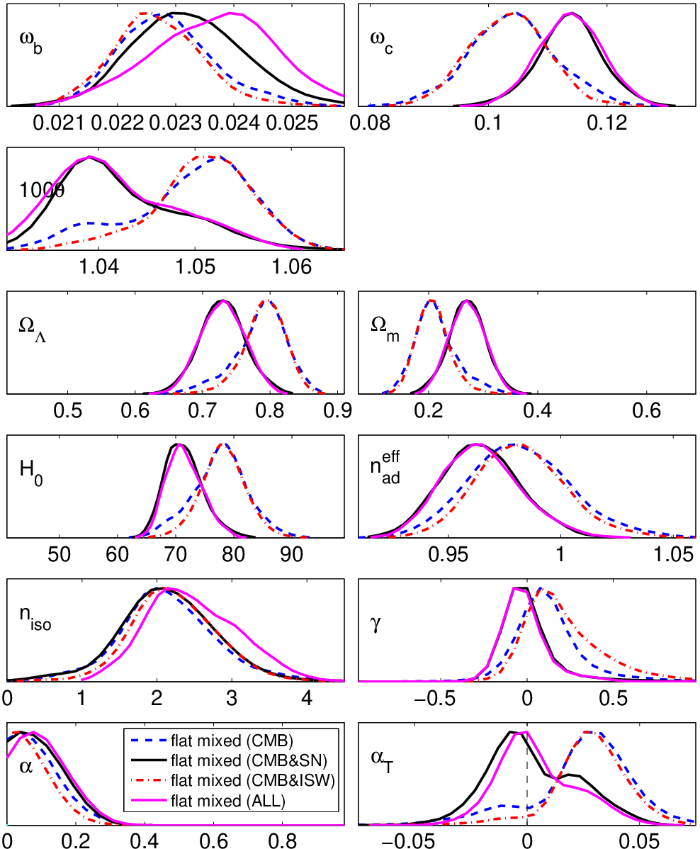
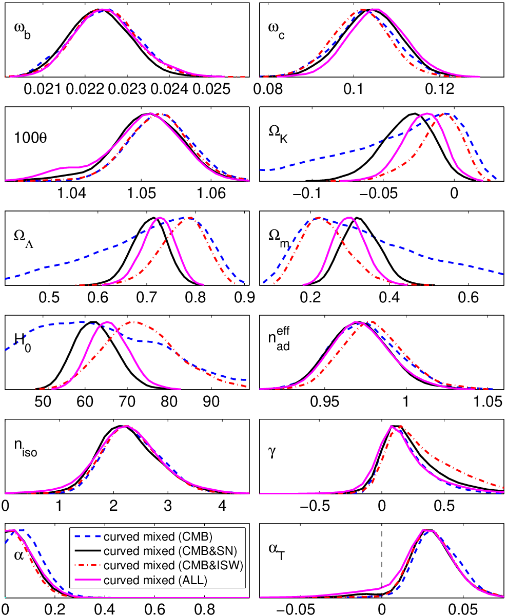
We study the likelihoods with various combinations of data, comparing the results to the adiabatic CDM model. First we use the CMB data alone, then we add either SN or ISW, and finally both of them into the analysis. We present 1d marginalised posterior likelihoods in the mixed model for the selected primary and derived parameters in Fig. 1 for the flat (left panel) and curved (right panel) cases.
IV.1 The CMB data alone
The CMB alone does favor a small amount of positively correlated isocurvature mode. This is consistent with what was previously reported in [48], although the few percent isocurvature contribution is now slightly less favored (over pure adiabatic model, ) due to the modified shape of the 2nd and 3rd acoustic peaks in the WMAP5 data.
The key points in Fig. 1 for the CMB data alone (blue dashed curves) are: mixed models with a small contribution from a CDM isocurvature mode, a small , a large , a large Hubble parameter , and a large sound horizon angle are marginally favored over the concordance adiabatic CDM model. The CMB favors a positive correlation, , between the primordial adiabatic and isocurvature perturbations (with the sign convention where a positive primordial correlation leads to a positive in the Sachs-Wolfe region, see e.g. [27, 48]). In the curved case a positive non-adiabatic contribution to the observed CMB temperature variance is more clearly favored than in the flat case. We find that at 98.9% (84.4%) CL in the curved (flat) case, or ( ) at 95% CL; see the bottom right plots in Fig. 1.
However, it is clear that due to the poorly constrained Hubble parameter, matter density, and curvature, we cannot use the current CMB data alone for studying the mixed model. Nevertheless, as we will discover in the next subsections, for a robust analysis it is crucial to know what are the favored regions in parameter space with the CMB data alone.

IV.2 Adding the SN and ISW data
Now we repeat the likelihood analysis with the CMB and SN data. In the flat case the data now prefer a purely adiabatic model: the likelihood of has a peak close to zero at slightly negative value. However, in the curved case adding the SN data hardly changes any of the likelihood distributions of isocurvature parameters (compare blue dashed and black solid curves in Fig. 1). Importantly the constraints of remain almost the same as with the CMB data alone: now at 95% CL.
The SN data do improve the constraints on some background parameters (, , , ), but do not significantly move the peaks of their likelihoods, in the curved case. As noticed above, the non-adiabatic contribution, , which is to some extent degenerate with and , stays untouched. We can understand this by looking at Fig. 2. The CMB tightly constrains the acoustic peak positions, and consequently the sound horizon angle , where is the sound horizon at last scattering and is the angular diameter distance to last scattering. As depends only on and , and even this dependence is very mild [77], the CMB constraint on is directly reflected by the favored , which depends on , (or ), and . The adiabatic model fits the acoustic peak positions perfectly whenever Mpc (indicated by the highlighted cyan curve in Fig. 2). However, in the mixed model there is an additional freedom caused by the ability of the correlated contribution to the angular power spectrum, , to move slightly the acoustic peak positions of the total toward right, as shown in figure 2 in Ref. [48]. Therefore a slightly larger , i.e. a smaller , is favored whenever there is a small positively correlated isocurvature contribution to the CMB. A Mpc (indicated by the highlighted magenta curve in Fig. 2) leads now to the best fits to the CMB. If we restrict the analysis to flat models (indicated by the thin black dashed line), the CMB picks the models (on the flat line, ) which are near the intersection point of the mentioned curve. In the adiabatic case this means (, ), whereas in the mixed case the intersection of Mpc and the flat line is at (, ). This explains why, in light of the CMB alone, the flatness assumption forces , (), and to quite unusual values, when allowing for the mixed initial conditions of perturbations.
If we now combine the CMB with SN (indicated by red dashed 95% CL curve in Fig. 2), it is clear that the well-fitting flat mixed models (the blue circle) will be excluded. However, in the curved case the SN data do not affect at all the well-fitting mixed models, and the best-fit region stays unaffected (the red diamond symbol). Finally, adding the ISW data (indicated by the blue dot-dashed 95% CL curve in Fig. 2) does not affect at all the well-fitting adiabatic or mixed models. Therefore the results for the isocurvature parameters with CMB&ISW are very close to the CMB alone case. The ISW data favor a slightly smaller matter density and slightly less closed Universe than the SN data, thus affecting these background parameters when compared to the CMB&SN analysis.
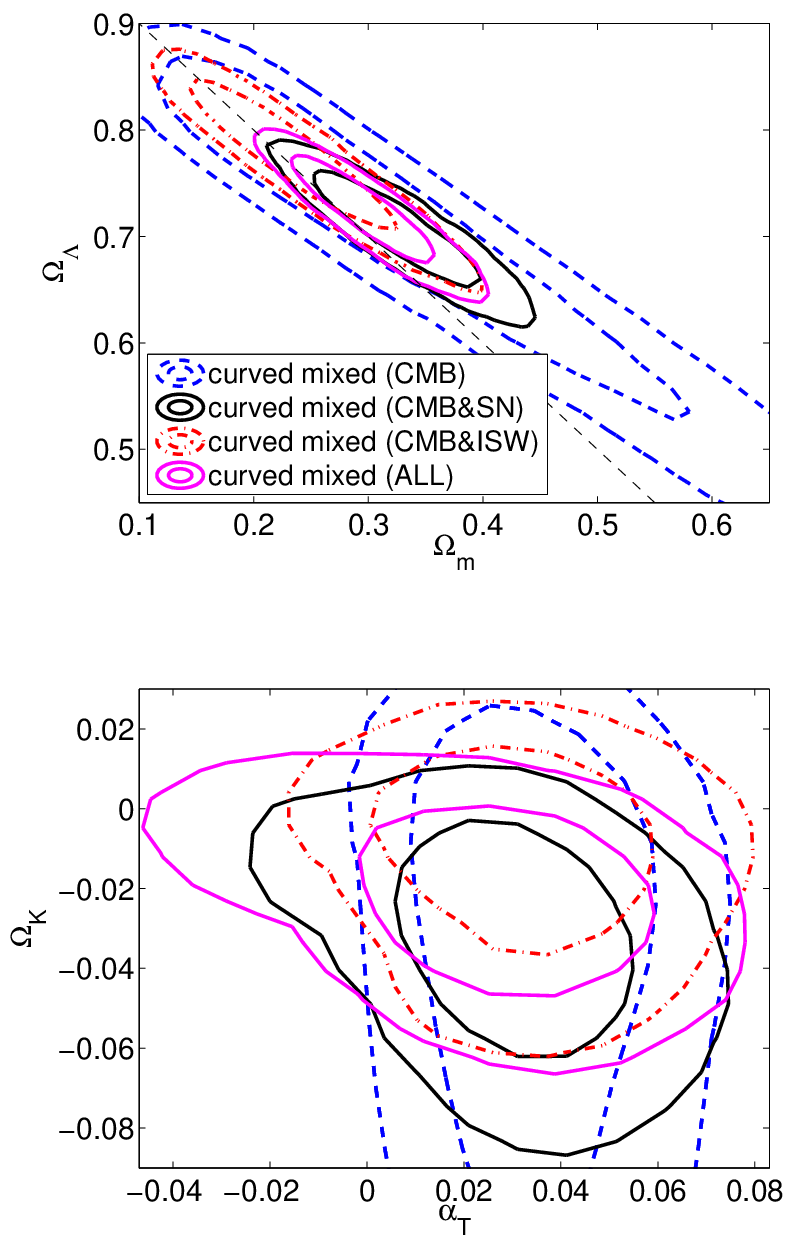
All the above remarks are confirmed by the 2d posterior likelihood contours shown in the upper panel of Fig. 3. The CMB alone leaves a long degeneracy line in the () plane for mixed models with Mpc. The SN or ISW data break this degeneracy, the ISW data favoring slightly lower than the SN data. Importantly, in the curved case, the well-fitting models to the CMB sit in the middle of the best-fit region of SN or ISW. Combining all the data (the magenta 68% and 95% CL curves) leads to the tightest constraints on and , being fully consistent with what we would expect from Fig. 2 and from the CMB&SN and CMB&ISW cases in Fig. 3.
The lower panel of Fig. 3 shows a tiny offset in the favored curvature between the SN and ISW data, and indicates why using all the data leads to looser constraints on , as seen in the bottom right plot in the right panel of Fig. 1.
The main conclusion after including the SN data is that, in the flat case, this brings the result in line with the concordance adiabatic model, as also reported in [28]. Here we must put once more emphasis on the fact that this happens only when restricting the analysis to flat models (thin black dashed lines in Figs. 2 and 3), whereas when allowing for spatial curvature of the Universe, a significant non-adiabatic contribution remains allowed. Most importantly, the well-fitting mixed models lie at the intersection of all the data (CMB, SN and ISW) at slightly closed geometry, though there is a slight competition (which exists also in the adiabatic case) between the higher value of preferred by the SN data, and the lower value preferred by the ISW data.
| Data | Model | |||||||||
|---|---|---|---|---|---|---|---|---|---|---|
| CMB&SN | flat adi | 3003.9 | — | 0.116 | 1.042 | — | 0.285 | 69.8 | 0.956 (0.932, 0.984) | — |
| flat mixed | 2999.0 | 0.002 (-0.03, 0.05) | 0.111 | 1.037 | — | 0.263 | 71.7 | 0.954 (0.930, 1.000) | 3.5 | |
| curved adi | 3002.4 | — | 0.107 | 1.042 | -0.03 (-0.04, 0.01) | 0.370 | 59.2 | 0.948 (0.934, 0.984) | — | |
| curved mixed | 2997.4 | 0.02 (0.00, 0.07) | 0.108 | 1.051 | -0.04 (-0.07, 0.00) | 0.380 | 58.5 | 0.967 (0.934, 1.009) | 2.9 |
IV.3 Robustness of the main cosmological parameters against the assumed initial conditions
An important question in constraining cosmologies is how much the assumptions made in the analysis affect the interpreted values of cosmological parameters from the given data [78]. Often pure adiabatic initial conditions are assumed when constraining the parameters of the CDM model. In this subsection we show how the favored values (or regions) of the main cosmological parameters change if one assumes mixed initial conditions. In other words, we answer the question “by assuming adiabaticity, would one find wrong constraints on the main cosmological parameters, if the underlying ’true’ initial perturbation mode happened to be a correlated mixture of adiabatic and CDM isocurvature perturbations?”.
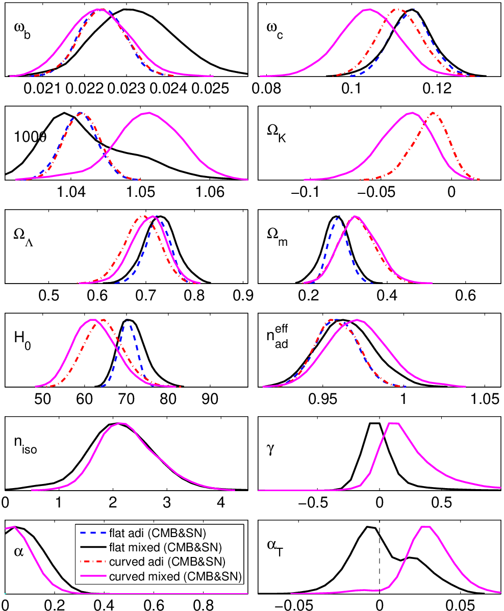
Obviously, using the CMB data alone leads to rather large differences between purely adiabatic and mixed models, in particular for the posterior likelihoods of , , , , (), , the age of the Universe, and . As it is unrealistic to assume tight constraints in the mixed model with CMB data alone, we demonstrate these effects in Fig. 4 with CMB&SN data.
In the flat case, the pure adiabatic model favors smaller values of , larger , slightly smaller (hence larger ), slightly smaller , and smaller . The CDM density remains unaffected. Interestingly, the scale-invariant primordial adiabatic perturbations, , are within the 95% CL region if mixed initial conditions are assumed, while being far in the tail of the posterior likelihood if pure adiabaticity is assumed.
In the curved case similar conclusions apply for and . However, since now the SN data do not exclude a few percent positively correlated non-adiabatic contribution in the closed models (with ) and these models are actually slightly favored over the flat adiabatic models, larger values of will be preferred compared to the pure adiabatic case. As explained in Sec. IV.2, the mixed model prefers a larger sound horizon angle, . This, together with the curvature, affects in turn and .
IV.4 Best fits and 95% CL intervals
To complete the discussion about the posterior likelihoods, we report in Table 2 the best-fit and selected best-fit parameters as well as 95% CL intervals for some of these with the CMB&SN data (as seen in Fig. 1, the CMB&ISW or CMB&SN&ISW data lead to very similar results). The between the best-fit flat mixed and flat adiabatic models is , while the difference between the curved models is . With the CMB alone these would be and , respectively. Noteworthy, the best-fit flat ’mixed’ model is almost adiabatic, whereas the best-fit curved mixed model has clearly non-zero isocurvature contribution — precisely as one would expect from the marginalized likelihoods.
As stated qualitatively in the previous subsection, the determination of spatial curvature and the adiabatic spectral index are significantly affected by the assumed initial conditions: assuming mixed initial conditions, a more closed geometry is favored than in the adiabatic case, and the flat geometry is excluded at 95% CL. On the other hand, the scale invariant primordial adiabatic spectrum is excluded at much more than 95% CL if adiabatic initial conditions are assumed, whereas — not surprisingly, due to the extra freedom to modify the shape of the total initial perturbation power spectrum — in the mixed models the 95% CL interval accommodates the scale invariant spectrum. This result contradicts the claim in Ref. [28] that the ’detection’ of red adiabatic spectrum () would be robust against the inclusion of the CDM isocurvature mode.
The 95% CL upper bound on the primordial contribution of the CDM isocurvature mode to the total perturbation power at the scale Mpc-1 is in the flat case, and in the curved case.
IV.5 Dependence on the pivot scale
We do not report any constraints for , since its posterior likelihood depends drastically on the chosen parametrization, in particular on the choice of the pivot scale, as shown in Fig. 5. While with some choices a scale invariant spectrum, , is ’allowed’, in general fairly large values () seem to be favored. There have not been many theoretical models that would predict such a large isocurvature spectral index, but recently an explicit axion model, which leads to —, was constructed in [79].
The posterior likelihoods obtained assuming flat priors in the amplitude parametrization (which we use for reporting the results in this paper), agree in general well with the more traditional spectral index parametrization, where flat priors for spectral indices and amplitudes at a pivot scale Mpc-1 are assumed. However, due to a different integration measure upon marginalization, the posterior likelihoods for all parameters differ from these, if we choose Mpc-1 or Mpc-1, which are the most common choices in the literature. In particular, the difference in the poorly constrained is large. This effect was first realized in [27], where it was strongly recommended that in the isocurvature analysis one should adopt Mpc-1, which leads to the tightest constraints and minimizes the ambiguity (caused by poorly constrained ) in determining the main cosmological parameters. As a further improvement, the amplitude parametrization, which we employ here, was suggested. With a large pivot scale (small ), a small appears to result in, whereas a small pivot scale (large ) leads to an apparent peak of the likelihood at . The most recent isocurvature analysis [28] suffers from this problem, since in [28] Mpc-1 is adopted. From Fig. 5 it is clear why [28] reports very loose constraints on , and claims that very large spectral tilts seem to be favored.
| Data | Model | ||||||
| Flat: adiabatic | Non-flat: adiabatic | Flat: mixed | Non-flat: mixed | ||||
| CMB | |||||||
| CMB&SN | |||||||
| — Sqrt param. | as above | as above | as above | ||||
| CMB&ISW | |||||||
| CMB&SN&ISW | |||||||
Apart from the issues with the spectral indices, our findings for the flat case agree well with [28] where the recent CMB (WMAP5 & ACBAR), SN (SNLS), and LSS (SDSS DR5 LRGs) data, and a Gaussian prior , were employed in flat models, without testing the results with individual combinations of the data, such as CMB&SN or CMB&LSS. Interestingly, based on comparing our results with those of [28], the LSS data do not seem to improve the constraints on the isocurvature. Moreover, the inclusion of LSS data is not enough to overcome the unsuitable choice of pivot scale made in [28], although one would have expected the LSS to improve the constraints on .
V Bayesian evidences
The main results of this paper, the Bayesian evidences (see e.g. Appendix A and Ref. [80]), are presented in Table 3. There we compare other models to the flat adiabatic CDM model, giving . Clearly the flat adiabatic CDM model is favored over curved adiabatic model and over both flat and curved mixed models. In light of the current data, the Bayesian model selection decisively () disfavors curved correlated isocurvature model. This is because the model selection punishes strongly for the 5 extra parameters (compared to the adiabatic CDM model) whose inclusion does not improve the fit to the data considerably: see, e.g., the bes-fit values for CMB&SN in Table 2. However, one should keep in mind that in the mixed models with , the main effect on the CMB is a modified 2nd and 3rd acoustic peak region. Therefore the determination of the isocurvature contribution is very sensitive to the calibration of the CMB temperature angular power spectrum in this region.
V.1 Evidences in an alternative parametrization
So far we have considered the primordial isocurvature perturbations in mixed models parametrized by the amplitudes and ( and ) of the primordial isocurvature (correlation) power spectrum at two different scales. It should be kept in mind that in Bayesian model selection, ’the model’ means the theoretical set-up including the chosen parametrization and the priors of these parameters. Therefore, by the very first principles of model selection, the evidences are inevitably sensitive to the chosen parametrization. To account for this, we reproduce a couple of our results for another mixed model, which is otherwise the same as the previous model, but where the primordial non-adiabatic components are described by amplitudes () of the primordial perturbations, instead of the amplitudes of the power spectra. These two parametrizations are related by
| (21) |
While the posterior likelihoods of the other cosmological parameters remain almost unchanged, and is affected by much less than , the different integration measure affects considerably the global Bayesian evidence. We show the evidences for our new mixed model, which we call ’sqrt parametrization’ or ’sqrt model’, in Table 3 for the CMB&SN data. In light of the CMB&SN data, the flat (curved) mixed sqrt model is within () from the flat adiabatic CDM model, corresponding to odds of 1:18 (1:33). Therefore, there is strong — but not decisive — evidence against the sqrt model. In particular, taking into account the error estimates of , the flat mixed sqrt model is not significantly disfavored when compared to the curved adiabatic CDM model. As their evidence difference corresponds to odds of 1:3, this suggests that in future studies, isocurvature should be treated on a similar footing as checking for curved adiabatic models.
VI Conclusions
In this paper we have presented a new likelihood and model selection analysis allowing for a correlated cold dark matter isocurvature mode of primordial perturbations, for the first time including spatial curvature.
Taking first a frequentist’s point of view, we have shown in the light of posterior likelihoods that models with a small fraction of isocurvature (%) are still favored by a CMB-only analysis, and including the Type Ia Supernovae or the integrated Sachs-Wolfe effect data does not change this result in the spatially curved Universe. Up to 7% positively correlated non-adiabatic contribution is allowed at 95% CL, whereas the pure adiabatic model lies near the boundary of the 95% CL region. In the flat case, we discover the previously known result that the SN data cut out the best-fit isocurvature models. Interestingly this does not happen in the curved case as indicated in Fig. 3. The ISW data constrain the vacuum energy density and curvature of the Universe in a complementary way to CMB or SN. Therefore the inclusion of the ISW data in the analysis sets more stringent constraints on the curvature, but does not seem to tighten the constraints on isocurvature.
We recommend including the spatial curvature in the isocurvature analysis of future CMB data (combined with some other probes of curvature, dark energy density, or Hubble parameter), since assuming flatness of the Universe considerably — and misleadingly — biases the results toward pure adiabaticity.
The Bayesian model selection, which heavily penalizes for any “unnecessary” extra degrees of freedom, disfavors strongly or decisively — depending on the parametrization of primordial perturbations — the mixture of correlated adiabatic and isocurvature primordial perturbations, in light of the current data. However, one should keep in mind that this result is very sensitive to the calibration of the CMB data around the second and third acoustic peaks, and therefore future data, e.g. from the Planck satellite, may either weaken or strengthen the constraints.
From a theoretical point of view, other scenarios that modify the second and third acoustic peak region typically involve other types of isocurvature, such as a dynamical contribution from cosmic strings [81]. In addition, the kinematic Sunyaev-Zel’dovich effect modifies the same region [82]. However, Planck should be able to distinguish between these and the mixed adibatic and CDM isocurvature model, since the former produce just a single ’bump’ of extra angular power, whereas the latter modifies the angular power spectrum in a more complex way at a few percent level, as shown in figure 2 in Ref. [48].
Although we have focused on isocurvature, we have also constrained the geometry of the Universe in the pure adiabatic model, finding that with the CMB&SN data the Bayesian model selection significantly (with odds of 1:6) disfavors spatially curved adiabatic model compared to the flat model. This constraint is tightened from ’significant’ to ’strong’ (with odds of 1:27) when we add the ISW data into the analysis.
It seems likely that the Bayesian model selection, with near-future data, could decisively rule out both the spatially curved geometry of the Universe and the mixed model, irrespectively of the parametrization issues, while the frequentist’s approach may continue to slightly ’favor’ these models over the flat CDM model.
However, it should be noticed that even the future CMB temperature anisotropy data alone are unlikely to constrain the mixed models with – better than the current WMAP data, as first pointed out in [83] (compare also figures 2c and 13 in [27], and see figure 1 in [55]). The reason is that on sub-horizon (sub-Hubble) scales before last scattering, the CDM density perturbations resulting from the primordial CDM isocurvature mode are damped by compared to those ones resulting from the adiabatic primordial mode. (Note that in the power spectrum this damping is , and in the angular power ). Therefore in order to significantly modify the predominantly adiabatic angular power spectrum above the multipole , one needs a large isocurvature spectral index. Consequently, models with would modify the anisotropy spectrum only at low multipoles, say , but here the temperature data are already now cosmic-variance limited. In particular, the future CMB temperature data can not significantly improve the constraints on a model where all the components share the same spectral index (), such as in [76]. Nevertheless, new accurate polarization data will help in reducing the uncertainty caused by the cosmic variance and in breaking the parameter degeneracies. Polarization data together with more accurate data on high multipoles also fix the background parameters better, leading indirectly to tighter constraints on isocurvature. As shown in [55], one can thus expect a moderate improvement on the constraints even for models with nearly scale-invariant isocurvature spectrum. Our main forecast, e.g., for Planck, is that having more accurate data on high multipoles, in particular helps to constrain the isocurvature spectral index in models where it could be (in this paper more than 50% of the well-fitting mixed models, see Fig. 1). In addition, Planck, as well as future supernovae data, will constrain the background parameters better and thus indirectly improve the constraints on the isocurvature contribution by breaking the degeneracies.
The prospects of the ISW data are more pessimistic. We have checked with our best-fit models that about 10 times more accurate ISW data would be needed if one was to directly discern between the perturbation spectra of the pure adiabatic and the mixed model, even with a large . Since the required accuracy is more than the theoretical bound for the signal to noise [67], the role of the ISW data will remain limited to constraining the background, and thus only indirectly the isocurvature contribution.
Acknowledgments
We thank Alessandro Melchiorri for suggesting us to work on this subject, and
we acknowledge the work and communications with
Reijo Keskitalo at the early stages of this project.
We thank the Bavarian Academy of Science and the Leibniz Computer Center in Munich, Germany, for computational resources.
In addition, a small part of the analysis was
performed at the Cosmos
supercomputer in Cambridge, United Kingdom. One of the cases
was run at the CSC, Finland. We thank the DEISA Consortium (www.deisa.eu), co-funded through the EU FP6
project RI-031513 and the FP7 project RI-222919, for support within the
DEISA Virtual Community Support Initiative.
JV was supported by Science and Technology Facilities Council (UK), and by the
Academy of Finland. TG acknowledges support from the Alexander von Humboldt Foundation.
References
- [1] M. R. Nolta et al. (WMAP), Astrophys. J. Suppl. 180, 296 (2009), eprint 0803.0593.
- [2] M. Kowalski et al. (Supernova Cosmology Project), Astrophys. J. 686, 749 (2008), eprint 0804.4142.
- [3] D. H. Lyth and A. Riotto, Phys. Rept. 314, 1 (1999), eprint hep-ph/9807278.
- [4] D. Polarski and A. A. Starobinsky, Phys. Rev. D50, 6123 (1994), eprint astro-ph/9404061.
- [5] M. Bucher, K. Moodley, and N. Turok, Phys. Rev. D62, 083508 (2000), eprint astro-ph/9904231.
- [6] D. H. Lyth and D. Wands, Phys. Lett. B524, 5 (2002), eprint hep-ph/0110002.
- [7] K. Enqvist and M. S. Sloth, Nucl. Phys. B626, 395 (2002), eprint hep-ph/0109214.
- [8] N. Bartolo and A. R. Liddle, Phys. Rev. D65, 121301 (2002), eprint astro-ph/0203076.
- [9] T. Moroi and T. Takahashi, Phys. Lett. B522, 215 (2001), eprint hep-ph/0110096.
- [10] F. Ferrer, S. Rasanen, and J. Valiviita, JCAP 0410, 010 (2004), eprint astro-ph/0407300.
- [11] M. Beltran, J. Garcia-Bellido, and J. Lesgourgues, Phys. Rev. D75, 103507 (2007), eprint hep-ph/0606107.
- [12] M. P. Hertzberg, M. Tegmark, and F. Wilczek, Phys. Rev. D78, 083507 (2008), eprint 0807.1726.
- [13] E. J. Copeland, J. E. Lidsey, and D. Wands, Nucl. Phys. B506, 407 (1997), eprint hep-th/9705050.
- [14] K. Koyama and D. Wands, JCAP 0704, 008 (2007), eprint hep-th/0703040.
- [15] A. Notari and A. Riotto, Nucl. Phys. B644, 371 (2002), eprint hep-th/0205019.
- [16] E. J. Copeland, J. B. Ellison, J. Roberts, and A. Lukas, Phys. Rev. D73, 086009 (2006), eprint hep-th/0601173.
- [17] K. Koyama and J. Soda, Phys. Rev. D65, 023514 (2002), eprint hep-th/0108003.
- [18] C. Tsagas and R. Maartens, Phys. Rev. D61, 083519 (2000), eprint astro-ph/9904390.
- [19] M. Giovannini, Class. Quant. Grav. 23, 4991 (2006), eprint astro-ph/0604134.
- [20] R. A. Battye and J. Weller, Phys. Rev. D61, 043501 (2000), eprint astro-ph/9810203.
- [21] T. Takahashi and M. Yamaguchi, Phys. Rev. D74, 063512 (2006), eprint hep-ph/0608115.
- [22] J. Valiviita, E. Majerotto, and R. Maartens, JCAP 0807, 020 (2008), eprint 0804.0232.
- [23] E. Majerotto, J. Valiviita, and R. Maartens (2009), eprint 0907.4981.
- [24] J. Valiviita, R. Maartens, and E. Majerotto (2009), eprint 0907.4987.
- [25] R. K. Sachs and A. M. Wolfe, Astrophys. J. 147, 73 (1967).
- [26] T. Giannantonio et al., Phys. Rev. D77, 123520 (2008a), eprint 0801.4380.
- [27] H. Kurki-Suonio, V. Muhonen, and J. Valiviita, Phys. Rev. D71, 063005 (2005), eprint astro-ph/0412439.
- [28] I. Sollom, A. Challinor, and M. P. Hobson, Phys. Rev. D79, 123521 (2009), eprint 0903.5257.
- [29] K. Enqvist, H. Kurki-Suonio, and J. Valiviita, Phys. Rev. D62, 103003 (2000), eprint astro-ph/0006429.
- [30] K. Enqvist, H. Kurki-Suonio, and J. Valiviita, Phys. Rev. D65, 043002 (2002), eprint astro-ph/0108422.
- [31] M. Beltran, J. Garcia-Bellido, J. Lesgourgues, and M. Viel, Phys. Rev. D72, 103515 (2005a), eprint astro-ph/0509209.
- [32] M. Beltran, J. Garcia-Bellido, J. Lesgourgues, A. R. Liddle, and A. Slosar, Phys. Rev. D71, 063532 (2005b), eprint astro-ph/0501477.
- [33] A. P. A. Andrade, C. A. Wuensche, and A. L. B. Ribeiro, Phys. Rev. D71, 043501 (2005), eprint astro-ph/0501399.
- [34] G. Lazarides, R. R. de Austri, and R. Trotta, Phys. Rev. D70, 123527 (2004), eprint hep-ph/0409335.
- [35] M. Beltran, J. Garcia-Bellido, J. Lesgourgues, and A. Riazuelo, Phys. Rev. D70, 103530 (2004), eprint astro-ph/0409326.
- [36] D. Parkinson, S. Tsujikawa, B. A. Bassett, and L. Amendola, Phys. Rev. D71, 063524 (2005), eprint astro-ph/0409071.
- [37] K. Moodley, M. Bucher, J. Dunkley, P. G. Ferreira, and C. Skordis, Phys. Rev. D70, 103520 (2004), eprint astro-ph/0407304.
- [38] J. Valiviita (2003), eprint astro-ph/0310206.
- [39] J. Valiviita and V. Muhonen, Phys. Rev. Lett. 91, 131302 (2003), eprint astro-ph/0304175.
- [40] J. Dunkley, M. Bucher, P. G. Ferreira, K. Moodley, and C. Skordis, Mon. Not. Roy. Astron. Soc. 356, 925 (2005a), eprint astro-ph/0405462.
- [41] A. P. Andrade, C. A. Wuensche, and A. L. B. Ribeiro, Astrophys. J. 602, 555 (2004), eprint astro-ph/0312028.
- [42] C. Gordon and K. A. Malik, Phys. Rev. D69, 063508 (2004), eprint astro-ph/0311102.
- [43] P. Crotty, J. Garcia-Bellido, J. Lesgourgues, and A. Riazuelo, Phys. Rev. Lett. 91, 171301 (2003), eprint astro-ph/0306286.
- [44] H. V. Peiris et al. (WMAP), Astrophys. J. Suppl. 148, 213 (2003), eprint astro-ph/0302225.
- [45] C. L. Bennett et al. (WMAP), Astrophys. J. Suppl. 148, 1 (2003), eprint astro-ph/0302207.
- [46] G. Hinshaw, D. N. Spergel, L. Verde, R. S. Hill, S. S. Meyer, C. Barnes, C. L. Bennett, M. Halpern, N. Jarosik, A. Kogut, et al., Astrophys. J. Supp. 148, 135 (2003).
- [47] M. Kawasaki and T. Sekiguchi, Prog. Theor. Phys. 120, 995 (2008), eprint 0705.2853.
- [48] R. Keskitalo, H. Kurki-Suonio, V. Muhonen, and J. Valiviita, JCAP 0709, 008 (2007), eprint astro-ph/0611917.
- [49] R. Trotta, Mon. Not. Roy. Astron. Soc. Lett. 375, L26 (2007), eprint astro-ph/0608116.
- [50] U. Seljak, A. Slosar, and P. McDonald, JCAP 0610, 014 (2006), eprint astro-ph/0604335.
- [51] A. Lewis (2006), eprint astro-ph/0603753.
- [52] R. Bean, J. Dunkley, and E. Pierpaoli, Phys. Rev. D74, 063503 (2006), eprint astro-ph/0606685.
- [53] G. Hinshaw, M. R. Nolta, C. L. Bennett, R. Bean, O. Doré, M. R. Greason, M. Halpern, R. S. Hill, N. Jarosik, A. Kogut, et al., Astrophys. J. Supp. 170, 288 (2007), eprint arXiv:astro-ph/0603451.
- [54] M. R. Nolta, J. Dunkley, R. S. Hill, G. Hinshaw, E. Komatsu, D. Larson, L. Page, D. N. Spergel, C. L. Bennett, B. Gold, et al., Astrophys. J. Supp. 180, 296 (2009), eprint 0803.0593.
- [55] J. Hamann, S. Hannestad, G. G. Raffelt, and Y. Y. Y. Wong, JCAP 0906, 022 (2009), eprint 0904.0647.
- [56] J. Dunkley, M. Bucher, P. G. Ferreira, K. Moodley, and C. Skordis, Phys. Rev. Lett. 95, 261303 (2005b), eprint astro-ph/0507473.
- [57] B. A. Bassett, P. S. Corasaniti, and M. Kunz, Astrophys. J. 617, L1 (2004), eprint astro-ph/0407364.
- [58] F. Feroz, M. P. Hobson, and M. Bridges (2008), eprint 0809.3437.
- [59] M. Vardanyan, R. Trotta, and J. Silk (2009), eprint 0901.3354.
- [60] C. Gordon, D. Wands, B. A. Bassett, and R. Maartens, Phys. Rev. D63, 023506 (2001), eprint astro-ph/0009131.
- [61] C. Gordon (2001), eprint astro-ph/0112523.
- [62] A. Lewis, A. Challinor, and A. Lasenby, Astrophys. J. 538, 473 (2000), eprint astro-ph/9911177.
- [63] A. Lewis and S. Bridle, Phys. Rev. D66, 103511 (2002), eprint astro-ph/0205436.
- [64] C. J. MacTavish et al., Astrophys. J. 647, 799 (2006), eprint astro-ph/0507503.
- [65] M. Cortes, A. R. Liddle, and P. Mukherjee, Phys. Rev. D75, 083520 (2007), eprint astro-ph/0702170.
- [66] C. L. Reichardt et al., Astrophys. J. 694, 1200 (2009), eprint 0801.1491.
- [67] R. G. Crittenden and N. Turok, Phys. Rev. Lett. 76, 575 (1996), eprint astro-ph/9510072.
- [68] J.-Q. Xia, M. Viel, C. Baccigalupi, and S. Matarrese, JCAP 0909, 003 (2009), eprint 0907.4753.
- [69] T. Giannantonio et al., Phys. Rev. D74, 063520 (2006), eprint astro-ph/0607572.
- [70] E. Gaztanaga, M. Manera, and T. Multamaki, Mon. Not. Roy. Astron. Soc. 365, 171 (2006), eprint astro-ph/0407022.
- [71] P.-S. Corasaniti, T. Giannantonio, and A. Melchiorri, Phys. Rev. D71, 123521 (2005), eprint astro-ph/0504115.
- [72] T. Giannantonio, Y.-S. Song, and K. Koyama, Phys. Rev. D78, 044017 (2008b), eprint 0803.2238.
- [73] L. Lombriser, W. Hu, W. Fang, and U. Seljak (2009), eprint 0905.1112.
- [74] T. Giannantonio, M. Martinelli, A. Silvestri, and A. Melchiorri (2009), eprint 0909.2045.
- [75] W. Percival, Private communication (2008).
- [76] R. Trotta, A. Riazuelo, and R. Durrer, Phys. Rev. D67, 063520 (2003), eprint astro-ph/0211600.
- [77] W. Hu, M. Fukugita, M. Zaldarriaga, and M. Tegmark, Astrophys. J. 549, 669 (2001), eprint astro-ph/0006436.
- [78] R. Trotta, A. Riazuelo, and R. Durrer, Phys. Rev. Lett. 87, 231301 (2001), eprint astro-ph/0104017.
- [79] S. Kasuya and M. Kawasaki, Phys. Rev. D80, 023516 (2009), eprint 0904.3800.
- [80] R. Trotta, Contemp. Phys. 49, 71 (2008), eprint 0803.4089.
- [81] N. Bevis, M. Hindmarsh, M. Kunz, and J. Urrestilla, Phys. Rev. Lett. 100, 021301 (2008), eprint astro-ph/0702223.
- [82] R. Genova-Santos, F. Atrio-Barandela, J. Muecket, and J. Klar, Astrophys. J. 700, 447 (2009), eprint 0905.2582.
- [83] J. Valiviita, The Nature of Primordial Perturbations in the Light of CMB Observations (Helsinki Institute of Physics, 2005), ISBN:952-10-1692-2, eprint http://urn.fi/URN:ISBN:952-10-1692-2.
- [84] J. Skilling, AIP conference proceedings of the 24th international workshop on Bayesian inference and maximum entropy methods in science and engineering (2004).
- [85] P. Mukherjee, D. Parkinson, and A. R. Liddle, Astrophys. J. 638, L51 (2006), eprint astro-ph/0508461.
- [86] R. Shaw, M. Bridges, and M. P. Hobson, Mon. Not. Roy. Astron. Soc. 378, 1365 (2007), eprint astro-ph/0701867.
- [87] F. Feroz and M. P. Hobson (2007), eprint 0704.3704.
Appendix A On the sampling technique
A.1 Bayesian inference
Bayesian statistics provides a good method to approach the two common problems of parameter estimation and model comparison. It is based on Bayes’ theorem which states that for a set of parameters , in a model , with data it holds
| (22) |
where the posterior probability distribution of the parameters is , the likelihood is , the prior is and the evidence is .
When estimating parameters for a given model, the standard practice is to ignore the evidence factor, and to estimate the posteriors using the standard MCMC method.
For model selection the evidence is instead crucial, since the ratio of evidences reflects the relative probabilities of the models. The evidence can be computed by the integration over all the dimensions of the parameter space
| (23) |
This expression incorporates automatically Occam’s principle of simplicity by penalizing models with extra parameters. When comparing two models and , the important quantity is the logarithmic difference in the evidences, also known as Bayes factor: . Then the model selection is qualitatively achieved using Jeffreys scale, which states that is not significant, is significant, is strong, and is decisive. In the main text we call as for clarity.
The standard method of thermodynamic integration, which is generally used to calculate the evidence, is very intensive and expensive, typically requiring the evaluation of the likelihoods for — models, and has been hindering the widespread use of Bayesian model comparison.
A.2 Nested sampling
The aforementioned problems are conveniently solved by the nested sampling method [84]. In this technique, the integral of Eq. (23) is replaced by a simpler 1-d integral
| (24) |
where the new variable represents the prior volume, identical to the parameter space volume in case of uniform priors, and is defined by , i.e.
| (25) |
where the integration is over the region contained in the iso-likelihood contour defined by . Thus the problem of calculating the evidence is reduced to the evaluation of the likelihoods at a series of points of decreasing value , so that the 1-d integration of Eq. (24) can be performed by summation as
| (26) |
where the weights can be given e.g. by a simple trapezoidal rule.
In more detail, the sampling of the can start with a uniform sampling of points (often called as ’live points’) within the priors, and then works its way up the likelihood surface by discarding at each iteration the lowest likelihood point and replacing it with a higher one. The process is terminated when some accuracy criterion is satisfied.
Once the evidence is known, the posteriors can be easily evaluated as a byproduct by using the set of points discarded at each iteration, giving each point a weight
| (27) |
A.3 MultiNest
After the conceptual introduction by [84], this method has been first applied to cosmology in a simple case by [85]. Its most sensitive part, the sampling technique, has been subsequently greatly refined by [86] and [87] to minimize the required number of likelihood evaluations and to deal efficiently with a series of possible pathologies, such as multi-modal posterior distributions and strongly curved parameter degeneracies.
Finally, an even more robust and efficient development has been released by [58] for applications in cosmology, astronomy and particle physics. The package, available for public use from http://www.mrao.cam.ac.uk/software/multinest, contains an easily usable interface for the CAMB/Cosmomc cosmology code [62, 63]. The user has simply to tune three parameters: the tolerance (accuracy), the number of live points , and the maximum efficiency , which sets how aggressively (or conservatively) we want the reduce the parameter space at each iteration. Another very attractive feature of this method is that any need of a proposal matrix for the parameters’ covariance, a well known hassle for MCMC users, is now completely superseded.
The analysis presented in this paper would have been impossible with the conventional MCMC method. With MultiNest, the curved cases, which were the toughest, took — CPUh each. The extensive comparisons presented in this paper took a total of CPUh, but this was doable in large super computers, since the MultiNest algorithm scaled linearly (with MPI parallelization) up to CPUs in our case and CAMB, which produces the theoretical predictions, scaled well up to — CPUs with openMP. An efficient configuration turned out to be 100 MPI 6 openMP threads in the main runs.
In most of the cases reported in this paper we set the efficiency parameter in MultiNest to 0.3, the tolerance (accuracy) parameter to 0.5, and the number of live points to .