Transform-based Distributed Data Gathering
Abstract
A general class of unidirectional transforms is presented that can be computed in a distributed manner along an arbitrary routing tree. Additionally, we provide a set of conditions under which these transforms are invertible. These transforms can be computed as data is routed towards the collection (or sink) node in the tree and exploit data correlation between nodes in the tree. Moreover, when used in wireless sensor networks, these transforms can also leverage data received at nodes via broadcast wireless communications. Various constructions of unidirectional transforms are also provided for use in data gathering in wireless sensor networks. New wavelet transforms are also proposed which provide significant improvements over existing unidirectional transforms.
Index Terms:
Data Compression, Wavelet Transforms, Wireless Sensor NetworksEDICS Category: SEN-DIST
I Introduction
In networks such as wireless sensor networks (WSNs), one major challenge is to gather data from a set of nodes and transfer it to a collection (or sink) node as efficiently as possible. Efficiency can be measured in terms of bandwidth utilization, energy consumption, etc. We refer to this as the data gathering problem. The gathering is typically done in data gathering rounds or epochs along a collection of routing paths to the sink, i.e., in every epoch each node forwards data that it has measured along a multi-hop path to the sink. A simple gathering strategy is to have each node route raw data to the sink in a way that minimizes some cost metric, e.g., number of hops to the sink, energy consumption. This minimizes the amount of resources nodes use to transfer raw data to the sink and is the basis for many practical systems used in WSN such as the Collection Tree Protocol (CTP) [1]. However, it has been recognized in the literature [2, 3] that, in a WSN, (i) spatial data correlation may exist across neighboring nodes and (ii) nodes that are not adjacent to each other in a routing path can still communicate due to broadcasted wireless transmissions11 1 Data transmissions in a WSN are typically broadcast [4, 5], so multiple nodes can receive a single data transmission.. Raw data forwarding does not make use of these two facts, thus, it will not be the most efficient data gathering method in general.
When spatial data correlation exists, it may be useful to apply in-network compression distributed across the nodes to reduce this data redundancy [2]. More specifically, nodes can exchange data with their neighbors in order to remove spatial data correlation. This will lead to a representation requiring fewer bits per measurement as compared to a raw data representation, also leading to reduced energy consumption, bandwidth usage, delay, etc. Since nodes in a WSN are severely energy-constrained [2, 3, 6], some form of in-network processing that removes data redundancy will help reduce the amount of energy nodes consume in transmitting data to the sink. In this way the lifetime of a WSN can be extended. This could also be useful in bandwidth-limited applications [7, 8].
Generally speaking, distributed spatial compression schemes require some form of data exchange between nodes. Therefore, one needs to select both a routing strategy and a processing strategy. The routing strategy defines what data communications nodes need to make and the processing strategy defines how each node processes data. There are a variety of approaches available, e.g., distributed source coding (DSC) techniques [9, 10], transform-based methods like Distributed KLT [11], Ken [12], PAQ [13], and wavelet-based approaches [14, 15, 16, 17, 18, 19, 20]. Note that DSC techniques do not require nodes to exchange data in order to achieve compression. Instead, each node can compress its own data using some statistical correlation model. Note, however, that an estimate of these models must be known at every node, so nodes will still need to do some initial data exchange in order to learn the models (after which compression can be done independently at each node). Our work only considers transform-based methods, which use linear transforms to decorrelate data while distributing transform computations across different nodes. While we do not consider DSC approaches, our algorithms could be useful in the training phase of these methods to estimate correlation. Ken and PAQ are examples of approaches we consider, where data at each node is predicted using a linear combination of measurements from the node and measurements received from its neighbors. Similarly, the Distributed KLT, wavelet-based methods and many other related methods also use linear transforms to decorrelate data. Therefore, we can restrict ourselves to linear in-network transforms while still encompassing a general class of techniques.
Many of the existing transform-based methods propose a specific transform first, then design routing and processing strategies that allow the transform to be computed in the network. Some examples are the wavelet transforms proposed in [14, 15, 18], the Distributed KLT, Ken and PAQ. While these methods are good from a data decorrelation standpoint, the routing and processing strategies that are used to facilitate distributed processing may not always be efficient in terms of data transport cost. In particular, nodes may have to transmit their own data multiple times [14, 15], nodes may need to transmit multiple copies of the same coefficients [18], or nodes may even need to transmit data away from the sink [11, 14, 15]. As discussed in [15], this sort of strategy can outperform raw data gathering for very dense networks, but it can lead to significant communication overhead for small to medium sized ones.
The results of our previous work [20, 21] and of [15] demonstrate why transport costs cannot be ignored. One simple way to work around these issues is to first design an efficient routing tree (e.g., a shortest path routing tree, or SPT), then allow the transform computations to occur only along the routing paths in the tree. We call these types of schemes en-route in-network transforms. These transforms (e.g., the wavelet transforms in [16, 17, 18, 19, 20]) will typically be more efficient since they are computed as data is routed to the sink along efficient routing paths. In addition to overall efficiency, these transforms can be easily integrated on top of existing routing protocols, i.e., a routing tree can be given by a protocol, then the transform can be constructed along the tree. This allows such schemes to be easily usable in a WSN - as demonstrated by the SenZip [22] compression tool, which includes an implementation of our algorithm in [20] - as well as other types of data gathering networks [7, 8].
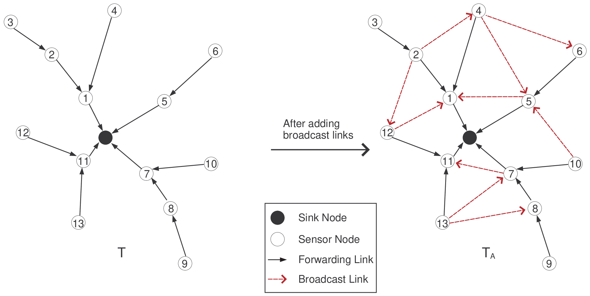
We note that all existing en-route transforms start from well-known transforms, then modify them to work on routing trees. Instead, in this work we start from a routing tree and additional links given by broadcast (e.g., Fig. 1). We then pose the following questions: (i) what is the full set of transforms that can be computed as data is routed towards the sink along and (ii) what are conditions for invertibility of these transforms? The main goal of this work is to determine this general set of invertible, en-route in-network transforms. Note that in many transform-based compression systems, design or selection of a transform is considered separately from the design of a quantization and encoding strategy. This is done in practice in order to simplify the system design (e.g., [23]). In general certain properties of the transform (energy compaction, orthogonality) can serve as indicators of achievable performance in the lossy case. We adopt a similar approach in our work, choosing to only focus on the transform design. Simple quantization and encoding schemes can then be applied to the transform coefficients, as demonstrated in our experimental results. Joint optimization of routing and compression is also possible, as in [24, 25] and our previous work [21], but this is beyond the scope of this work.
In order to formulate this problem, we first note that the data gathering process consists of data measurement at each node and routing of data to the sink along done in accordance with some transmission scheduling, i.e., nodes transmit data along in a certain order. Also note that data is only transmitted along in the direction of the sink, i.e., data transmissions are unidirectional towards the sink. Moreover, each node can only process its own data with data received from other nodes that transmit before it, i.e., processing of data must be causal in accordance with the transmission schedule. In particular, before each node transmits it will only have access to data received from nodes that use it as a relay in a multi-hop path to the sink (i.e., “descendants”) and nodes whose data it receives but is not responsible for forwarding to the sink (i.e., “broadcast” neighbors). Whenever broadcast is used, data from a single node will often be available at multiple nodes. While this can help to decorrelate data even further (since more data will be available for transform computations at each node), it would be undesirable to transmit this same piece of data through multiple paths since this would increase the overall communication cost. Thus, in addition to causality and unidirectionality, the transform should also be critically sampled, i.e., the number of transform coefficients that are computed and routed to the sink is equal to the number of nodes in the network. We refer to causal, critically-sampled transforms that are computed in a unidirectional manner as unidirectional transforms.
As we will show, unidirectional transforms can be defined in terms of the routing tree, the broadcast links induced by the routing and the transmission schedule. Thus, given a tree and transmission schedule, the main problem we address in this work is to determine a set of necessary and sufficient conditions under which an arbitrary unidirectional transform is invertible. While unidirectional transforms have been proposed, to the best of our knowledge, none of the existing works have attempted to define the most general set of unidirectional transforms, nor has any attempt been made to find conditions under which such transforms are invertible. Our proposed theory also incorporates the use of broadcast data in a general setting. This leads us to develop transforms that use broadcasts in a manner not previously considered. This contribution is discussed in detail in Section II.
In the context of wavelet transforms for WSNs, early work [16, 17, 18, 19] developed unidirectional wavelet transforms on 1D routing paths in WSNs. Extensions to 2D routing paths on arbitrary routing trees were made by the authors in [20, 21]. The superiority of these 1D [18] and 2D [20] transforms over the method in [15] (which requires a great deal of backward communication) was demonstrated in [20]. General unidirectional transforms were initially proposed by us in [26], in the context of lifting transforms [27], and conditions for single-level invertible unidirectional lifting transforms were initially proposed there. However, no invertibility conditions were provided for general unidirectional transforms, nor were any conditions given for invertible multi-level unidirectional lifting transforms. We provide such conditions here (Section II and III-C) as well as new transform designs (Section IV) which outperform our previously proposed transforms.
General unidirectional transforms with a set of necessary and sufficient invertibility conditions are presented in Section II. In order to demonstrate the generality of our proposed theory, Section III shows how existing unidirectional transforms (e.g., the tree-based KLT [28], tree-based differential pulse code modulation (T-DPCM) [28, 22] and lifting transforms [26, 28]) can be mapped into our framework. Moreover, our proposed formalism is used to construct general unidirectional lifting transforms. Some of the inefficiencies of existing lifting transforms are then discussed. In order to address these inefficiencies, we define a new Haar-like wavelet transform in Section IV which is analogous to the standard Haar wavelet when applied to 1D paths. As is shown in Section IV, our formalization guarantees invertibility of these Haar-like transforms, and also leads to an extension which incorporates broadcast. Section V provides experimental results that demonstrate the benefits of using our proposed transforms.
II En-route In-network Transforms
In this section, assuming a fixed routing tree and schedule are given, we provide a definition of unidirectional transforms and determine conditions for their invertibility. Some notation is established in Section II-A. Unidirectional transforms are then defined in Section II-B. Section II-C presents a set of conditions under which these transforms are invertible. Throughout this discussion, the configuration of the network in terms routing and scheduling is assumed to be known. Section II-D addresses how this can be achieved in practice and how our approach can be used with decentralized initialization approaches.
II-A Notation
Assume there are nodes in the network with a given routing tree , where , each node is indexed by , the sink node is indexed by , and denotes an edge from node to node along . We also assume that there is a graph which is defined by the edges in and any additional edges that arise from the broadcast nature of wireless communications. An example graph is shown on the right side of Fig. 1. We observe that data gathering consists of three key components. The first is data measurement, where each node measures some scalar data that it must send to the sink in each epoch (these ideas can be easily generalized to non-scalar data22 2 One straightfoward extension is to use a “separable” transform, where a transform is first applied in one dimension (e.g., over time or across dimensions of a multivariate input) and then in the other (i.e., spatially).). Additionally, node must route its data to the sink along . The tree is defined by assigning to every node a parent . We assume that these trees are provided by a standard routing protocol such as CTP. Finally, we assume that data transmissions are scheduled [4, 29] in some manner, i.e., node will transmit data to its parent at time according to a transmission schedule (see Definition 1). CTP is a practical example that can be viewed in terms of this formalization: nodes are assigned parents in a distributed manner, data is forwarded to the sink along the corresponding routing paths and the times at which nodes transmit serve as an implicit transmission schedule.
Definition 1 (Transmission Schedule)
A transmission schedule is a function , such that when node transmits in the -th time slot33 3 Note that these time slots are not necessarily of equal length; they simply allow us to describe the order in which communications proceed in the network; before time slot , node is listening to other nodes, and at time node starts transmitting its own data, and potentially data from its descendants in the routing tree.. Moreover, node transmits data before node whenever .
Note that, along the tree , each node has a set of descendants which use node as a data relay to the sink and a set of ancestors that node uses for relaying data to the sink. Moreover, we only consider to be descendants of those nodes that are descendants on the tree and transmit earlier than . Also let each node be hops away from the sink node, i.e., has depth in . We also let denote the descendants of which are exactly hops away from , i.e., , where is the -th ancestor of node (e.g., is the parent of , is the grandparent of , etc). For instance, is the set of children of , is the set of grandchildren of , etc, and for simplicity we let . Also note that data can be heard via broadcast in many networks (e.g., WSNs), so we let define the full set of broadcast neighbors whose data node can overhear due to broadcast.
Under this formulation, each node can process its own data together with data received from and . This yields transform coefficient for node and transform coefficients for its descendants, i.e., for all . We make an abuse of notation by letting . Note that node is only responsible for forwarding and to its parent , thus, it should not transmit any data received from broadcast neighbors. In particular, we assume that node transmits the transform coefficient vector to its parent at time . We refer to this as critical-sampling, where in each epoch only one transform coefficient per sample per node is generated and then transmitted to the sink. In our formulation, we also allow (and ) to be further processed at the ancestors of . We refer to this type of processing as delayed processing.
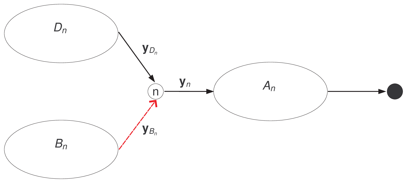
Note that data is only transmitted along towards the sink, i.e., data relay is unidirectional towards the sink. The existence of a transmission schedule - given explicitly or implicitly - also induces a notion of causality for transform computations. In particular, the computations performed at each node can only involve and any received from a node that transmits data before node . More specifically, nodes can only use data from if (we assume that for all ). These constraints (i.e., causality and unidirectional relay) induce causal neighborhoods whose data each node can use for processing, where we let denote the set of causal broadcast neighbors. These can be abstracted as in Fig. 2 where and . These are formally defined as follows.
Definition 2 (Causal Neighborhoods)
Given a routing tree and schedule , the causal neighborhood of each node is the union of the descendants and the set of causal broadcast neighbors , i.e., . We also define for future discussions.
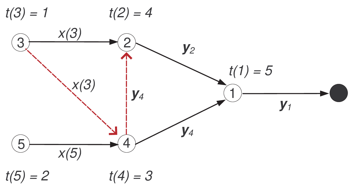
These ideas are illustrated in Fig. 3. For instance, when node 2 forwards data to node 1, its communication is also overheard by nodes 4 and 12. However, nodes 4 and 12 will not receive data from node 2 before they transmit, thus, they cannot use it for processing.

II-B Definition of Unidirectional Transforms
We define a unidirectional transform (not necessarily invertible) as any transform that (i) is computed unidirectionally along a tree and (ii) satisfies causality and critical sampling. Now we can establish the general algebraic form of unidirectional transforms. Without loss of generality, assume that node indices follow a pre-order numbering [30] on , i.e., for all (see Fig. 3 for an example of pre-order numbering). A pre-order numbering always exists, and can be found via standard algorithms [30]. For the sake of simplicity, we also assume that the transmission schedule provides a unique time slot to each node44 4 We note that the time slot assignment need not be unique. However, this assumption significantly simplifies the transform construction and invertibility conditions. It is easy to develop similar transform constructions when multiple nodes are assigned the same time slots, and similar invertibility conditions arise., i.e., for all .
Recall that each node receives and from its descendants and (causal) broadcast neighbors, respectively (see Fig. 2). Thus, in a general unidirectional transform, each node processes its own data along with and . Then, it will transmit transform coefficient vector at time . We omit from the notation of since the timing is implicit. In order to satisfy critical-sampling, it is necessary that each node only forward coefficients to the sink. Therefore, must be a dimensional vector. A unidirectional transform can now be expressed as follows.
Definition 3 (Unidirectional Transform)
Let be a routing tree with a unique time slot assignment given by , and suppose that the causal neighborhood of each node is given by Definition 2. A unidirectional transform on is a collection of local transformations done at each node given by
| (1) |
where has dimension , has dimension and each has dimension . The transform is computed starting from the node at the first time slot up through the nodes in the remaining time slots .
II-C Invertibility Conditions for Unidirectional Transforms
We now establish a set of invertibility conditions for unidirectional transforms. Note that these transforms are always computed in a particular order, e.g., starting from nodes furthest from the sink (i.e., “leaf” nodes), up to nodes which are 1-hop from the sink. Some sort of interleaved scheduling (where one set of nodes transmits before the rest) could also be used [31]. Therefore, it would also be desirable to have step by step decoding in the reverse order, since this would simplify the transform constructions. In particular, if the overall transform can be inverted by inverting the computations done at each node in the reverse order, then invertibility will be ensured by designing invertible transforms at each node.
Step by step decoding in the reverse order is trivially guaranteed when no broadcast data is used since the transform at each node is simply . Thus, if each is invertible, we can invert the operations done at node as . This becomes more complicated when broadcast data is used. By examining (1), we observe that , where . In order to have step by step decodability, we need to be able to recover (for every node ) and from and . Note that this fails whenever we cannot decode some transform coefficient vector from broadcast node before decoding . It will also fail if the matrix operations performed at any given node are not invertible. Thus, in order to guarantee step by step decodability, we need to ensure that (i) the matrix operations at each node are invertible, and (ii) it is possible to decode each before decoding . As we now show, (i) is guaranteed by ensuring that each matrix is invertible and (ii) is guaranteed by imposing a timing condition.
Proposition 1 (Step by Step Decodability)
Suppose that we have the transform in Definition 3 and assume that for every broadcast node . Then we can recover and as if and only if exists.
Proof:
Note that the vector transmitted by any broadcast node will be processed at its parent, node , and this processing will occur at time . Moreover, node will generate its own transform coefficient vector at time , and by assumption we have that . Thus, it is possible to decode before for every broadcast neighbor . Thus, we can always form before decoding . Therefore, we can recover and as if and only if exists. ∎
To simplify our transform constructions, we also assume that nodes use the latest version of broadcast data that they receive, i.e., only if . This second constraint precludes the possibility that a node receives broadcast data from node and from an ancestor of node . Removing the broadcast links which violate these constraints gives a simplified communication graph as shown on the right side of Fig. 3. Removal of these links can be done by local information exchange within the network; examples of how this can be achieved are discussed in Section II-D. Under the constraint of Prop. 1 and this second constraint, we can represent the global transform taking place in the network as follows. Since the time slot assignment is unique, at time only data from and its descendants will be modified, i.e., only and will be changed at time . Since pre-order indexing is used, we have that . Therefore, the global transform computations done at time are given by (2), where each corresponds to data which is not processed at time .
| (2) |
The global transform matrix at time is just the matrix shown in (2), i.e.,
| (3) |
This yields the global transform coefficient vector
| (4) |
Fig. 4 illustrates these transform computations. Initially, . At times 1 and 2, nodes 3 and 5, respectively, transmit raw data to their parents. Therefore, the global matrices at times 1 and 2 are simply . At time 3, node 4 produces
where and represent arbitrary values of the transform matrix used at node 4. Then at time 4, node 2 produces transform coefficients and (and coefficient vector ) as
where and are the values of the matrix used at node 2. Node 1 then computes at time 5. The global transform is given by
| (5) |
It is now rather simple to show that the transform is invertible as long as each matrix is invertible.
Proposition 2 (Invertible Unidirectional Transforms)
Proof:
Under the two broadcast timing assumptions, the global transform is given by (4). (4) is invertible if and only if every in (3) is invertible. is invertible if and only if . Recall that adding a multiple of one row to another does not change the determinant [32]. Given the structure of the matrices, using such row operations to eliminate each matrix, it is easy to show that . Moreover, Prop. 1 implies that is invertible. ∎
Proposition 2 shows that locally invertible transforms provide globally invertible transforms. Moreover, under our stated timing constraints, broadcast data does not affect invertibility. Therefore, broadcast data at each node can be used in an arbitrary manner without affecting invertibility. So in order to design an invertible unidirectional transform, all that one must do is design invertible matrices . This is an encouraging result since it essentially means that broadcast data can be used in any way a node chooses. In particular, broadcast data can always be used to achieve more data decorrelation.
II-D Discussion
The theory presented thus far assumes that the routing and transmission scheduling are known, and that all of the transform matrices are known both at the nodes and at the sink. In practice, the routing, scheduling and transforms must be initialized. Moreover, the network may need to re-configure itself if, for example, nodes die or link conditions change drastically. In addition, packet losses will often occur. Nodes typically deal with this (as in CTP) by re-transmitting a packet until an acknowledgement (ACK) is received from the intended recipient. While these three issues pose no significant problems for routing, they all have an impact on our proposed transform due to the assumptions we make about timing. We now provide some discussion of how this affects our theory and how it can be handled.
We first address the impact that initialization and reconfiguration have on the routing and scheduling, as well as what can be done to address it. We assume that routing is initialized and reconfigured in a distributed manner using standard protocols such as CTP. Distributed scheduling protocols for WSNs also exist [29, 33]. However, the resulting schedules may not be consistent with Definition 2 (i.e., they may not provide timings for which for all ), so in practice we would need to enforce such timings. One way to achieve this is to force nodes to suppress transmission (in a given epoch) until they have received data from all of their descendants. Another alternative would be to determine such a transmission schedule at the sink, then to disseminate the timing information to the nodes.
Whenever timing and routing information is established (or re-established due to re-configuration), it is also necessary to check our main broadcast timing constraint, i.e., only if . We describe one way in which this information can be disseminated to each node in a distributed manner. First, whenever the time at node is initialized or changes, it broadcasts a small packet (i.e., a beacon) which contains to its children. Then, any child of which broadcasts data will send the same beacon to all of its neighbors. This requires a total of 2 messages for each broadcasting node. Note that protocols such as CTP already use control beacons (in addition to data packets) to update stale routing information. Thus, nodes could potentially piggyback timing information on these control beacons whenever they are generated, or otherwise use separate control beacons to disseminate timing information. This will incur an additional cost, although (as was shown in [1]) the per packet cost for control beacons is typically much smaller than the cost for data forwarding.
Initialization and re-configuration also impacts the transform matrices that are used. Each node could transmit the values of its matrix to the sink, or viceversa, but this may be very costly. Instead, the construction of each transform matrix should be based on a small amount of information which is made common to the nodes and to the sink. For example, the values in each transform matrix could be based on the number of 1-hop neighbors that each node has [20] or the relative node positions [14]. In this way each matrix can be constructed at each node and at the sink without explicitly communicating the matrix values. However, additional information (e.g., node positions, number of neighbors) would need to be communicated to the sink whenever the network is initialized or re-configured. For example, each node could construct a transform using only the number of nodes that it receives data from (as in [20, 14]) and would send the set of nodes whose data it used as overhead to the sink. Then, assuming that the nodes and the sink construct the matrices according to the same rules, the sink can re-construct the matrix used at each node.
Packet loss is the last practical issue which impacts our proposed transforms. We do not consider the effects of channel noise on the data since these can be handled using a wide variety of existing techniques. Moreover, packet losses and channel noise will impact other data gathering schemes (e.g., CTP), and we expect that the penalty due to packet losses will be similar in our scheme and in other data gathering schemes. Packet losses are typically handled (as in CTP) by re-transmitting a packet until an ACK is received from the desired destination. Thus, if node does not receive data from descendant by the time that it transmits, due to packet re-transmissions for , the data from node cannot be combined with data available at node . This is equivalent to not using the data from node in the transform computation (i.e., for all and ) and does not affect our proposed theory. However, this change must be signaled to the sink so that it knows how to adjust accordingly. This can be done by including some additional information in the packet headers for node and to signify this change.
Packet losses also have an impact on the use of broadcast data. Suppose that node does not receive a data packet from broadcast neighbor but the packet from does reach the intended recipient . In this case, node will send an ACK back to node and node will no longer re-transmit (note that node will not expect an ACK from node ). Thus, data from node can not be combined with data available at node . This is equivalent to not using data from node in the transform computation (i.e., ) and our proposed theory is not affected. However, this change must be signaled to the sink so that it knows to set .
One way to work around these issues (initialization, re-configuration and packet losses) is to design transforms that can work under arbitrary timing and with arbitrary uses of broadcast data. However, under arbitrary timing and use of broadcast data, it is no longer possible to guarantee global transform invertibility by designing invertible transforms at each node. More specifically, we must ensure that the transform computations done at different nodes are jointly invertible. This leads to a set of complex conditions. The cost to determine such conditions and to coordinate nodes so that they satisfy these conditions could be very high, perhaps even much higher than the additional coordination needed to implement our proposed transforms. However, it is still possible to design simple versions of such transforms by using constructions such as lifting. Our recent work [31] is one particular example. Given this high degree of complexity to ensure an invertible transform when using broadcast, broadcast data should probably only be used with our proposed transforms if (i) it is possible to fix the timing in the network in accordance with the Definition 2, and, (ii) the timing is very stable.
III Unidirectional Transform Designs
Proposition 2 provides simple conditions for invertible transform design, i.e., is invertible for every node . This is a simple design constraint that unifies many existing unidirectional transforms. In this section, we demonstrate how existing unidirectional transforms can be mapped to our formulation. In particular, we focus on the tree-based Karhunen-Loève Transform (T-KLT) [28], T-DPCM [22, 28] and early forms of tree-based wavelet transforms [16, 17, 18, 20] constructed using lifting [27].
In order to exploit spatial correlation to achieve reduction in the number of bits per measurement, nodes must first exchange data. Therefore, some nodes must transmit raw data to their neighbors before any form of spatial compression can be performed. Since raw data typically requires many more bits than encoded transform coefficients, it would be desirable to minimize the number of raw data transmissions that nodes must make to facilitate distributed transform computation. Therefore, our main design consideration is to minimize the number of raw data transmissions that are required to compute the transform.
III-A Tree-based Karhunen-Loève Transform
Since transforms that achieve data decorrelation potentially lead to better coding efficiency [34], we consider now the design of unidirectional transforms that achieve the maximum amount of data decorrelation. This can be achieved by applying, at each node , a transform that makes all of the coefficients in statistically uncorrelated (or “whitened”), e.g., by using a Karhunen-Loève transform (KLT) at each node, leading to the T-KLT described in our previous work [28]. In this transform, each node computes and transmits a set of “whitened” coefficients , which will then have to be “unwhitened” and then re-whitened at to produce a new set of whitened coefficients. Whitening can be done using a KLT and unwhitening can be achieved using an inverse KLT. More specifically, this is done at each node by (i) finding the whitening transform and unwhitening transforms of each child , (ii) applying an unwhitening transform to each child to recover the original measurements as , and then (iii) rewhitening these measurements as . This transform (without quantization) can then be expressed in terms of our formulation as
| (6) |
with . Each is trivially invertible since and each are invertible by construction. Therefore, the tree-based KLT is trivially invertible.
III-B Tree-based DPCM
A simpler alternative to the T-KLT is T-DPCM [22, 28]. A related DPCM based method was proposed in [35]. This particular method is not designed for any particular communication structure, but it can easily be adapted to take the form of a unidirectional transform. In contrast to the method in [35], the T-DPCM methods in [22, 28] compute differentials directly on a tree such as an SPT.
In the T-DPCM method of [28], each node computes its difference with respect to a weighted average of its children’s data, i.e., . For this to be possible, one of two things must happen: either every node must decode the differentials received from its children to recover for each , or, every node must transmit raw data two hops forward to its grandparent (at which point can be computed) to avoid decoding data at every node. In order to avoid each node having to forward raw data two hops, at each node , the inverse transform on the data of each child must be computed first using the inverse matrix of each child. The forward transform is then designed accordingly. We can express this version of T-DPCM as in (7).
| (7) |
The matrix is just the product of these triangular matrices, hence, it is trivially invertible. Moreover, only leaf nodes need to forward raw data and the rest transmit only transform coefficients.
Alternatively, in the T-DPCM scheme of [22], each node first forwards raw data to its parent , then node computes a differential for and forwards it to the sink, i.e., node computes . This transform can also be mapped to our formalism as
| (8) |
This eliminates the computational complexity of the previous T-DPCM method since no decoding of children data is required. However, every node must now forward raw data one hop. Moreover, it will not decorrelate the data as well as the first method since only data from one neighbor is used.
III-C Unidirectional Lifting-based Wavelets
We now describe how unidirectional wavelet transforms can be constructed under our framework. This can be done using lifting [27]. Lifting transforms are constructed by splitting nodes into disjoint sets of even and odd nodes, by designing prediction filters, which alter odd data using even data, and update filters, which alter even data based on odd data. They are invertible by construction [27].
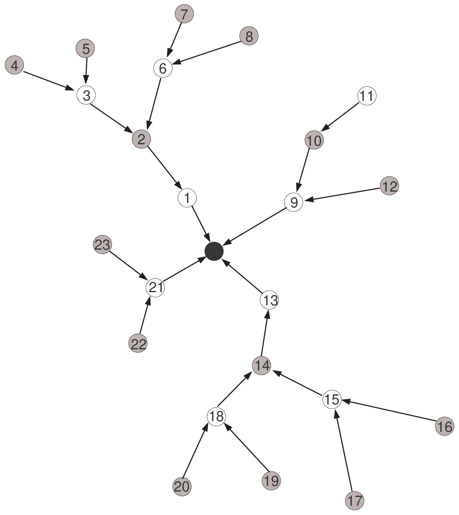
First, nodes are split into odd and even sets and , respectively. This can be done completely arbitrarily. One example from our previous work [20] is to split according to the depth in the tree, e.g., and , as illustrated in Fig. 5. Data at each odd node is then predicted using data from even neighbors , yielding detail coefficient
| (9) |
The prediction vector can provide a simple average [20], i.e., for each , a planar prediction [15] of the data at node using data from its neighbors, or can even be data adaptive [28]. Incorporating some broadcast data into the prediction is also useful since it allows odd nodes to achieve even further decorrelation. After the prediction step, data at each even node is updated using details from odd neighbors , yielding smooth coefficient
| (10) |
The update vector can provide simple smoothing [20], i.e., for all , or could provide orthogonality between smooth (i.e., low-pass) and detail (i.e., high-pass), coefficients [36].
By the lifting construction, invertibility will be guaranteed as long as (i) odd node data is only predicted using even node data, and (ii) even node data is only updated using details from odd nodes. So if and is an arbitrary even and odd split, the transform computed at each node will be invertible as long as the computations satisfy (i) and (ii). More formally, let be the set of odd nodes whose data is available at from its subtree. Let be defined similarly. Moreover, let denote the set of odd nodes whose data receives via broadcast. Similarly, let . Then the computations at will be invertible as long as it only predicts from and and only updates from and . Let and be permutation matrices such that
| (11) |
Then can compute transform coefficients as in (12).
| (12) |
By multiplying the matrices in (11) and (12) together, we get , with
Since , single-level unidirectional lifting transforms are always invertible.
The transform given by (12) corresponds to only one level of decomposition. In particular, at each node the transform of (12) will yield a set of smooth (or low-pass) coefficients and a set of detail (or high-pass) coefficients . The high-pass coefficients will typically have low energy if the original data is smooth, so these can be encoded using very few bits and forwarded to the sink without any further processing. However, there will still be some correlation between low-pass coefficients. It would therefore be useful to apply additional levels of transform to the low-pass coefficients at node to achieve more decorrelation. This will reduce the number of bits needed to encode these low-pass coefficients, and will ultimately reduce the number of bits each node must transmit to the sink.
Suppose each node performs an additional levels of lifting transform on the low-pass coefficients . At each level , suppose that nodes in are split into even and odd sets and , respectively. We assume that . For each odd node , we predict using even coefficients from some set of even neighbors , i.e., . Then for each even node , we update using odd coefficients from some set of odd neighbors , i.e., . This decomposition is done starting from level up to level . For all , let be a permutation matrix such that
| (13) |
where is the set of nodes whose coefficients are not modified at level . Then we can express the level transform computations in matrix form as
| (14) |
where and represent the prediction and update operations used at level , respectively.
By combining (11), (12), (13) and (14), we finally get that , with and defined in (15) and (16).
| (15) |
| (16) |
Prop. 2 implies that the overall transform is invertible if given in (15) is invertible. Since each is a permutation matrix, . Moreover, the remaining matrices are triangular. Thus, it easily follows that . Therefore, unidirectional, multi-level lifting transforms are always invertible.
III-D Unidirectional 5/3-like Wavelets
Our previous work [20] provides a 5/3-like transform on a tree. First, nodes are split into odd and even sets and , respectively, by assigning nodes of odd depth as odd and nodes of even depth as even. More specifically, and . This is illustrated in Fig. 5. The transform neighbors of each node are simply for every node . This provides a 5/3-like wavelet transform on a tree since whenever averaging predictions and smoothing updates are used along a 1D path, the transform reduces to the 5/3 wavelet transform [37]. Nodes can compute these transforms in a unidirectional manner, but doing so requires that some nodes forward raw data 1 or 2 hops. This is illustrated in Fig. 6.
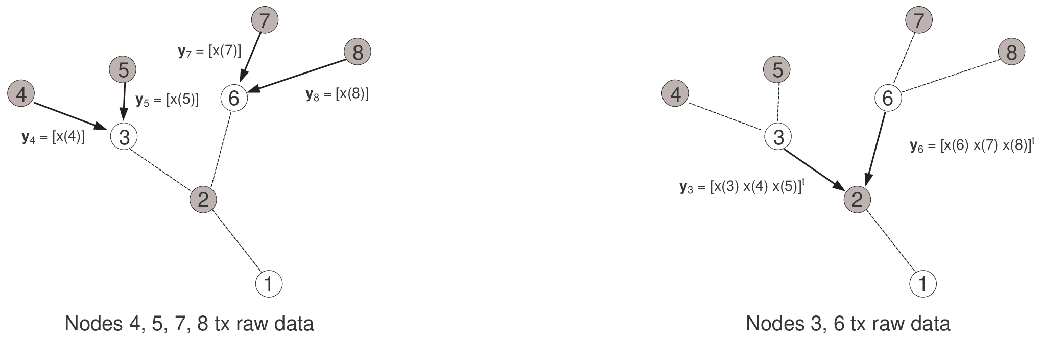
Data from each odd node is predicted using data (from children ) and (from parent ). However, odd node will not have locally available for processing. Therefore, we require that each odd node transmit raw data one hop forward to its parent , at which point node can compute the detail coefficient of . Each even node will then compute detail for every child . Similarly, the smooth coefficient of each even node requires details from its parent and children , so it can not be locally computed either. Moreover, detail can only be computed at node , i.e., at the grandparent of . Therefore, we require that even node transmit raw data two hops forward to , at which point will be available and can compute . Note that each of these operations are trivially invertible, and easily lead to local transform matrices which are invertible by construction. However, the number of raw data transmissions is relatively high, i.e., 1-hop for odd nodes and 2-hops for even nodes. We address this inefficiency in the next section.
IV Unidirectional Haar-like Wavelets
For the transform in Section III-D, raw data from even and odd nodes must be forwarded over 2-hops and 1-hop, respectively. This can be inefficient in terms of transport costs. Instead, it would be better to construct a lifting transform which directly minimizes the number of raw data transmissions each node must make. We use the splitting method in Section III-D. Note that some form of data exchange must occur before the transform can be computed, i.e., evens must transmit raw data to odds, or viceversa. Suppose that even nodes forward raw data to their parents. In this case, the best we can do is to design a transform for which even nodes transmit raw data over only 1-hop, and odd nodes do not transmit any raw data. This will minimize the number of raw data transmissions that nodes need to make, leading to transforms which are more efficient than the 5/3-like transform in terms of transport costs. We note that minimizing raw data only serves as a simple proxy for the optimization. A more formal optimization which relies on this same intuition is undertaken in our recent work [31].
IV-A Transform Construction
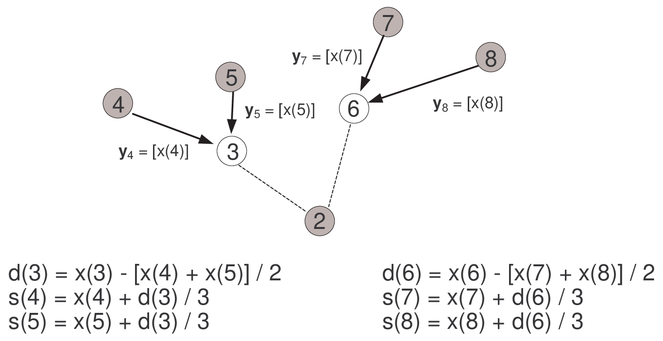
A design that is more efficient than the 5/3-like transform can be achieved as follows. Note that an odd node has data from its children and/or even broadcast neighbors locally available, so it can directly compute a detail coefficient for itself, i.e., . Thus, the detail is computed directly at , is encoded, and then is transmitted to the sink. These details require fewer bits for encoding than raw data, hence, this reduces the number of bits that odd nodes must transmit for their own data. Since data from even node is only used to predict data at its parent , we simply have that and . Moreover, these smooth coefficients can be computed at each odd node . Therefore, even nodes only need to forward raw data over one hop, after which their smooth coefficients can be computed. Note that not all odd nodes will have children or even broadcast neighbors, i.e., there may exist some odd nodes such that and . Such odd nodes can simply forward raw data to their parent , then can compute their details as . Thus, there may be a few odd nodes that must send raw data forward one hop. This leads to a Haar-like transform which is exactly the Haar wavelet transform when applied to 1D paths.
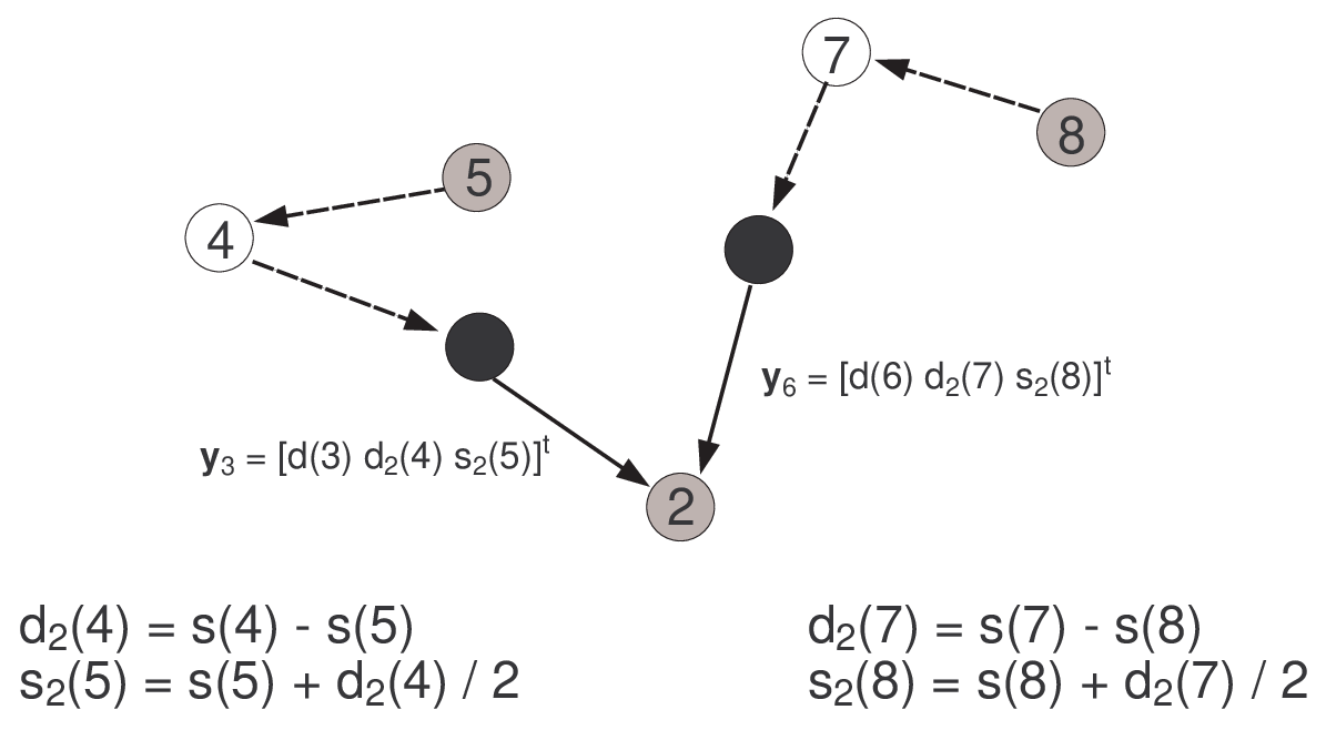
Odd nodes can also perform additional levels of decomposition on the smooth coefficients of their descendants. In particular, every odd node will locally compute the smooth coefficients of its children. Therefore, it can organize the smooth coefficients onto another tree and perform more levels of transform decomposition along . In this work, we assume is a minimum spanning tree. This produces detail coefficients , , , and smooth coefficients for some . In this way, odd nodes can further decorrelate the data of their children before they even transmit. This reduces the resources they consume in transmitting data. An example of this separable transform for is illustrated in Fig. 7. By choosing averaging prediction filters and the orthogonalizing update filter design in [36], we get the global equation in (17).
| (17) |
The coefficient vector is obtained in a similar manner. More generally, these sorts of multi-level transform computations can always be formulated into matrices as described in Section III-C.
IV-B Discussion
The transform computations that each node performs can be easily mapped into our standard form by appropriately populating the matrices in (15) and (16). Therefore, they will always yield invertible transforms. For example, since each odd node predicts its own data using data from its children and even broadcast neighbors , then updates the data of its children from its own detail, the operations for a single level transform at odd can be expressed as
| (18) |
By choosing
| (19) |
and
| (20) |
we have that . Note that (18) covers all of the cases discussed in Section IV-A for each odd node , that is to say: (i) and , (ii) and , (iii) and , and (iv) and . In particular, whenever , and will have some non-zero entries. Otherwise, has no descendants and so and will just be vectors of zeros. Similarly, whenever , will have some non-zero entries. Otherwise, has no even broadcast neighbors and will be a vector of zeros.
Similarly, each even node may need to compute predictions for its odd children, so its computations for a single level transform can be expressed as
| (21) |
Also note that (21) covers all of the cases for each even node discussed in Section IV-A, i.e., when has to compute predictions for children then , otherwise, .
Note that, when broadcast data is used, the decorrelation achieved at odd nodes may still be comparable to the 5/3-like transform since the same number of neighbors (or more) will be used. Moreover, broadcasts are particularly useful for odd nodes that have no children, i.e., for which but . If broadcast data is not used when it is available, node will have to transmit to its parent. Since requires more bits for encoding than does a detail coefficient , will consume more resources during data transmission. By using broadcasts, these odd nodes which have no children can still use data overheard from even broadcast neighbors, allowing them to avoid transmitting raw data to their parents. This is illustrated in Fig. 8, where node 11 has no children but overhears data from node 12. The example in Fig. 8(a) will consume more resources at node 11 than will the example in Fig. 8(b).


V Experimental Results
This section presents experimental results that compare the transforms proposed here against existing methods. Source code used to generate these results can be found on our webpage55 5 http://biron.usc.edu/wiki/index.php/Wavelets_on_Trees. In particular, we focus on comparing the proposed multi-level Haar-like lifting transforms against the multi-level 5/3-like transform from [20, 26], the T-DPCM scheme in [28] and raw data gathering. We consider the application of distributed data gathering in WSNs. Performance is measured by total energy consumption.
V-A Experimental Setup
For evaluation, we consider simulated data generated from a second order AR model. This data consists of two 2D processes generated by a second order AR model with low and high spatial data correlation, e.g., nodes that are a certain distance away have higher inter-node correlation for the high correlation data than for the low correlation data. More specifically, we use the second order AR filter , with and (resp. ) to produce data with low (resp. high) spatial correlation. The nodes were placed in a grid, with node measurements corresponding to the data value from the associated position in the grid. Each network used in our simulations is generated from a set of random node positions distributed in the grid. An SPT is constructed for each set of node positions. We consider two types of networks: (i) variable radio range networks in which each node can have a diferent radio range, and (ii) fixed radio range networks in which each node has the same radio range. In the variable radio range case, the radio range that each node uses for transmission is defined by the distance from to its parent in the SPT. Additional broadcast links induced by the SPT are also included, i.e., a broadcast link between node and exists if is not a direct neighbor of in the SPT but is within radio range of .
In order to measure energy consumption, we use the cost model for WSN devices proposed in [6, 38], where the energy consumed in transmitting bits over a distance is Joules and the energy consumed in receiving bits is Joules. The terms capture the energy dissipated by the radio electronics to process bits. The term captures the additional energy for signal amplification needed to ensure reasonable signal power at the receiver. WSN devices also consume energy when performing computations, but these costs are typically very small compared with transmission and reception costs. Therefore, we ignore them in our cost computations. Also note that all data gathering schemes will suffer from channel noise and attenuation, so a no-channel-loss comparison is still valid. Thus, we do not consider these effects in our experiments.
Comparisons are made with the Haar-like transforms of Section IV against the 5/3-like transform with delayed processing proposed in [26] and the T-DPCM scheme proposed in [28]. Predictions for each of these transforms are made using the adaptive prediction filter design in [28]. Updates are made using the “orthogonalizing” update filter design in [36]. In each epoch, we assume that each node transmits measurements taken at different times. Also, each raw measurement is represented using bits. We assume each odd node encodes detail coefficients together with an adaptive arithmetic coder. Smooth coefficients are treated like raw data, i.e., each one uses bits. Since we only seek to compare the performance of spatial transforms, we do not consider any temporal processing.
V-B Simulation Results
In the case of lossless compression, the average cost reduction ratios taken over multiple uniformly distributed networks are shown in Fig. 9 for high and low data correlation. These are expressed as the average of multiple values of , where is the cost for joint routing and transform and is the cost for raw data forwarding. Results for variable radio ranges (each node has different radio range) are shown in Fig. 9(a). Results for fixed radio ranges (each node has the same radio range) are given in Fig. 9(b). T-DPCM does the worst overall. The 5/3-like transform provides significant improvement over the simple T-DPCM scheme. The Haar-like transforms have the highest average cost reduction ratio, or equivalently, the lowest average cost. Moreover, we note that broadcast is not very helpful (on average) when nodes have variable radio ranges (Fig. 9(a)), but there is a significant gain when nodes use a fixed radio range (Fig. 9(b)). This is mainly because, in the fixed radio range case, (i) there are many more opportunities for using broadcast data and (ii) each node has more broadcast neighbors.


Note that the amount of raw data forwarding needed to compute the Haar-like transform is significantly reduced compared with the 5/3-like transform. Therefore, the Haar-like transform will do better than the 5/3-like transform in terms of transport costs. Granted, the 5/3-like transform will use data from more neighbors for processing, so the decorrelation given by the 5/3-like transform will be greater than that given by the Haar-like transform. However, in our experiments the average reduction in rate that the 5/3-like transform provides over the Haar-like transform is rather small. The Haar-like transform with broadcast also provides additional cost reduction over the Haar-like transform without broadcasts since less raw data forwarding is needed on average. Moreover, the amount of cost reduction achievable is higher for the high correlation data than for the low correlation data.
Lossy coding is also possible and can provide even greater cost reductions while introducing some reconstruction error. In this case, we quantize transform coefficients with a dead-zone uniform scalar quantizer. Performance is measured by the trade-off between total cost and distortion in the reconstructed data, which we express as the signal to quantization noise ratio (SNR). Sample 50 node networks are shown in Figs. 10(a) and 10(c) and, in the case of high correlation data, the corresponding performance curves are shown in Figs. 10(b) and 10(d). The Haar-like transforms do the best among all transforms.


When using broadcasts with the Haar-like transform, there is an additional 1 dB (resp. 2.5 dB) gain in SNR for the variable (resp. fixed) radio range network at a fixed cost, i.e., by using broadcasts we can increase the quality in the reconstructed data for a fixed communication cost. Thus, for these networks, using broadcast is quite helpful. Also note that there only 2 broadcast links used in the transform for the variable radio range network (Fig. 10(a)), whereas there are over 10 broadcast links used in the fixed radio range network (Fig. 10(c)). Thus, broadcast provides even greater gains for the fixed radio range network (2.5 dB versus 1dB) since there are more broadcast links. More generally, broadcast should provide more gains in networks where many broadcast opportunities are available.
Also note that in this particular network for the variable radio range case, T-DPCM actually does better than the 5/3-like transform. Note that in T-DPCM, only the leaf nodes forward raw data to the sink; so if there are only a few leaf nodes, the raw data forwarding cost for T-DPCM may not be very high compared with the raw data forwarding cost for the 5/3-like transform. In this particular network, only 19 of the 50 nodes are leaves in the tree. Therefore, the raw data forwarding cost for T-DPCM in this case is lower than that for the 5/3-like transform. However, on average the raw data forwarding cost for T-DPCM will be very high (see Fig. 9), leading to higher total cost on average as compared with the 5/3-like transform.
VI Conclusions
A general class of en-route in-network (or unidirectional) transforms has been proposed along with a set of conditions for their invertibility. This covers a wide range of existing unidirectional transforms and has also led to new transform designs which outperform the existing transforms in the context of data gathering in wireless sensor networks. In particular, we have used the proposed framework to provide a general class of invertible unidirectional wavelet transforms constructed using lifting. These general wavelet transforms can also take into account broadcast data without affecting invertibility. A unidirectional Haar-like transform was also proposed which significantly reduces the amount of raw data transmissions that nodes need to make. Since raw data requires many more bits than encoded transform coefficients, this leads to a significant reduction in the total cost. Moreover, our proposed framework allows us to easily incorporate broadcasts into the Haar-like transforms without affecting invertibility. This use of broadcast data provides further performance improvements for certain networks.
References
- [1] O. Gnawali, R. Fonseca, K. Jamieson, D. Moss, and P. Levis, “Collection tree protocol,” in SenSys ’09, November 2009.
- [2] C. Chong and S. P. Kumar, “Sensor networks: Evolution, opportunities, and challenges,” Proceedings of the IEEE, vol. 91, no. 8, pp. 1247–1256, August 2003.
- [3] I.F. Akyildiz, W. Su, Y. Sankarasubramaniam, and E. Cayirci, “A survey on sensor networks,” IEEE Communication Magazine, vol. 40, no. 8, pp. 102–114, August 2002.
- [4] I. Cidon and M. Sidi, “Distributed assignment algorithms for multi-hop packet-radio networks,” IEEE Transactions on Computers, vol. 38, no. 10, October 1989.
- [5] W. Ye, J. Heidemann, and D. Estrin, “An energy-efficient MAC protocol for wireless sensor networks,” in INFOCOM ’02, 2002.
- [6] A. Wang and A. Chandraksan, “Energy-efficient DSPs for wireless sensor networks,” IEEE Signal Processing Magazine, vol. 19, no. 4, pp. 68–78, July 2002.
- [7] J.G. Proakis, E.M. Sozer, J.A. Rice, and M. Stojanovic, “Shallow water acoustic networks,” IEEE Communications Magazine, vol. 39, no. 11, pp. 114–119, 2001.
- [8] K. Mechitov, W. Kim, G. Agha, and T. Nagayama, “High-frequency distributed sensing for structure monitoring,” in In Proc. First Intl. Workshop on Networked Sensing Systems (INSS), 2004.
- [9] R. Cristescu, B. Beferull-Lozano, and M. Vetterli, “Networked Slepian-Wolf: Theory, algorithms, and scaling laws,” IEEE Transactions on Information Theory, vol. 51, no. 12, pp. 4057–4073, December 2005.
- [10] S.S. Pradhan, J. Kusuma, and K. Ramchandran, “Distributed compression in a dense microsensor network,” IEEE Signal Processing Magazine, pp. 51–60, March 2002.
- [11] M. Gastpar, P. Dragotti, and M. Vetterli, “The distributed Karhunen-Loève transform,” IEEE Transactions on Information Theory, vol. 52, no. 12, pp. 5177–5196, December 2006.
- [12] D. Chu, A. Deshpande, J. Hellerstein, and W. Hong, “Approximate data collection in sensor networks using probabilistic models,” in IEEE International Conference on Data Engineering (ICDE). 2006, pp. 3–7, IEEE.
- [13] D. Tulone and S. Madden, “PAQ: Time series forecasting for approximate query answering in sensor networks,” in Proceedings of the European Conference in Wireless Sensor Networks (EWSN). Feb. 2006, pp. 21–37, IEEE.
- [14] R. Wagner, H. Choi, R. Baraniuk, and V. Delouille, “Distributed wavelet transform for irregular sensor network grids,” in IEEE Stat. Sig. Proc. Workshop (SSP), July 2005.
- [15] R. Wagner, R. Baraniuk, S. Du, D.B. Johnson, and A. Cohen, “An architecture for distributed wavelet analysis and processing in sensor networks,” in IPSN ’06, April 2006.
- [16] J. Acimovic, B. Beferull-Lozano, and R. Cristescu, “Adaptive distributed algorithms for power-efficient data gathering in sensor networks,” Intl. Conf. on Wireless Networks, Comm. and Mobile Computing, vol. 2, pp. 946–951, June 2005.
- [17] A. Ciancio and A. Ortega, “A flexible distributed wavelet compression algorithm for wireless sensor networks using lifting,” in Proc. of ICASSP’04, 2004.
- [18] A. Ciancio, S. Pattem, A. Ortega, and B. Krishnamachari, “Energy-efficient data representation and routing for wireless sensor networks based on a distributed wavelet compression algorithm,” in IPSN ’06, April 2006.
- [19] A. Ciancio, Distributed Wavelet Compression Algorithms for Wireless Sensor Networks, Ph.D. thesis, University of Southern California, 2006.
- [20] G. Shen and A. Ortega, “Optimized distributed 2D transforms for irregularly sampled sensor network grids using wavelet lifting,” in Proc. of ICASSP’08, April 2008.
- [21] G. Shen and A. Ortega, “Joint routing and 2D transform optimization for irregular sensor network grids using wavelet lifting,” in IPSN ’08, April 2008.
- [22] S. Pattem, G. Shen, Y. Chen, B. Krishnamachari, and A. Ortega, “Senzip: An architecture for distributed en-route compression in wireless sensor networks,” in Workshop on Sensor Networks for Earth and Space Science Applications (ESSA), April 2009.
- [23] D. Taubman and D. Marcellin, JPEG2000: Image Compression Fundamentals, Standards and Practice, Kluwer Academic Publishers, 1st edition, 2001.
- [24] S. Pattem, B. Krishnamachari, and R. Govindan, “The impact of spatial correlation on routing with compression in wireless sensor networks,” ACM Transactions on Sensor Networks, vol. 4, no. 4, pp. 60–66, August 2008.
- [25] P. Rickenbach and R. Wattenhofer, “Gathering correlated data in sensor networks,” in Proceedings of the 2004 Joint Workshop on Foundations of Mobile Computing, October 2004.
- [26] G. Shen, S. Pattem, and A. Ortega, “Energy-efficient graph-based wavelets for distributed coding in wireless sensor networks,” in Proc. of ICASSP’09, April 2009.
- [27] W. Sweldens, “The lifting scheme: A construction of second generation wavelets,” Tech. report 1995:6, Industrial Mathematics Initiative, Department of Mathematics, University of South Carolina, 1995.
- [28] G. Shen, S. Narang, and A. Ortega, “Adaptive distributed transforms for irregularly sampled wireless sensor networks,” in Proc. of ICASSP’09, April 2009.
- [29] K. Sohrabi, J. Gao, V. Ailawadhi, and G. J. Pottie, “Protocols for self-organization of a wireless sensor network,” IEEE Personal Communications, vol. 7, no. 5, October 2000.
- [30] G. Valiente, Algorithms on Trees and Graphs, Springer, 1st edition, 2002.
- [31] S.K. Narang, G. Shen, and A. Ortega, “Unidirectional graph-based wavelet transforms for efficient data gathering in sensor networks,” in Proc. of ICASSP’10, March 2010.
- [32] G. Strang, Linear Algebra and its Applications, Thomson Learning, 3rd edition, 1988.
- [33] A. Sridharan and B. Krishnamachari, “Max-min fair collision-free scheduling for wireless sensor networks,” in Proc. of IEEE IPCCC Workshop on Multi-hop Wireless Networks, April 2004.
- [34] V.K. Goyal, “Theoretical foundations of transform coding,” IEEE Signal Processing Magazine, vol. 18, no. 5, pp. 9–21, September 2001.
- [35] H. Luo, Y.C. Tong, and G. Pottie, “A two-stage DPCM scheme for wireless sensor networks,” in Proc. of ICASSP’05, March 2005.
- [36] G. Shen and A. Ortega, “Tree-based wavelets for image coding: Orthogonalization and tree selection,” in Proc. of PCS’09, May 2009.
- [37] S. Mallat, A Wavelet Tour of Signal Processing, Elsevier, 2nd edition, 1999.
- [38] W. R. Heinzelman, A. Chandrakasan, and H. Balakrishnan, “Energy-efficient routing protocols for wireless microsensor networks,” in Proc. of Hawaii Intl. Conf. on Sys. Sciences, January 2000.