On the magnetic equation of state in (2+1)-flavor QCD
Abstract
A first study of critical behavior in the vicinity of the chiral phase transition of (2+1)-flavor QCD is presented. We analyze the quark mass and volume dependence of the chiral condensate and chiral susceptibilities in QCD with two degenerate light quark masses and a strange quark. The strange quark mass () is chosen close to its physical value; the two degenerate light quark masses () are varied in a wide range , where the smallest light quark mass value corresponds to a pseudo-scalar Goldstone mass of about 75 MeV. All calculations are performed with staggered fermions on lattices with temporal extent . We show that numerical results are consistent with scaling in the chiral limit. We find that in the region of physical light quark mass values, , the temperature and quark mass dependence of the chiral condensate is already dominated by universal properties of QCD that are encoded in the scaling function for the chiral order parameter, the magnetic equation of state. We also provide evidence for the influence of thermal fluctuations of Goldstone modes on the chiral condensate at finite temperature. At temperatures below, but close to the chiral phase transition at vanishing quark mass, this leads to a characteristic dependence of the light quark chiral condensate on the square root of the light quark mass.
pacs
11.15.Ha, 12.38.GcI Introduction
Chiral symmetry and its spontaneous breaking in the vacuum are key ingredients to our understanding of the phase structure of strongly interacting matter at non-zero temperature and vanishing baryon chemical potential. In the limit of massless quark flavors the QCD phase transition is controlled by the chiral symmetry. Quite general renormalization group arguments suggest [1] that QCD with three degenerate light quark flavors has a first order phase transition, whereas the 2-flavor theory is expected to have a second order phase transition. In the latter case the chiral symmetry is isomorphic to and the transition therefore is expected to belong to the same universality class as 3-dimensional, symmetric spin models. Depending on the value of the strange quark mass the QCD phase transition in the limit of vanishing light quark masses (up, down) may be first order or a continuous transition still belonging to the 3-dimensional, universality class [1].
While numerical calculations in 3-flavor QCD gave evidence for the existence of a first order transition, many of the details of the transition in 2- or (2+1)-flavor QCD with light up and down quarks are still poorly constrained through lattice calculations. In particular, we do not know whether the chiral phase transition in (2+1)-flavor QCD is first or second order. An answer to this question is not only of academic interest; it also greatly influences our thinking about the phase diagram of QCD at non-zero baryon chemical potential [2]. The present analysis, although still performed on rather coarse lattices, is a first step towards answering this question.
Attempts to verify the universal critical behavior associated with the QCD chiral phase transition in 2-flavor QCD have been made already before in calculations with staggered [3, 4, 5, 7, 6, 8, 9] and Wilson [10, 11] fermions. None of these lattice discretization schemes for the fermion sector of QCD preserve the full chiral symmetry of the QCD Lagrangian. It therefore may not be too surprising that the early attempts to verify universal scaling properties of QCD were not too successful. In fact, at non-zero lattice spacing the Wilson fermion formulation does not preserve any continuous symmetry related to the chiral sector of QCD. The staggered formulation preserves at least an symmetry at non-zero lattice spacing that gives rise to a single massless Goldstone mode in the chiral limit. Nevertheless, direct determinations of critical exponents within the staggered discretization scheme [3, 4, 7] did not deliver the expected results. Of course, due to the explicit breaking of symmetry in the staggered formalism at non-vanishing lattice spacing one would not have expected to be sensitive to scaling. However, and critical exponents are quite similar and one thus might have hoped to observe at least some generic evidence for scaling11 1 We are dealing here with numerical calculations of a cutoff theory whose Lagrangian has a global symmetry. The relevant symmetry of QCD in the continuum limit, on the other hand, is expected to be . For many aspects of the discussion of critical behavior presented here, the distinction between and is of no importance. In these cases we will generically talk about symmetric models..
In the same spirit, the magnetic equation of state, i.e. the scaling of the chiral order parameter as function of reduced temperature and quark mass, has been analyzed subsequently in calculations with staggered [5, 6, 8] and Wilson fermions [10, 11]. The studies performed with Wilson fermions gave some indication for scaling. These calculations, however, had been constrained to the high temperature, symmetry restored phase and had been performed with rather large values of the quark mass. They therefore did not allow to perform a test of scaling in the symmetry broken phase and could not contribute to the question of how Goldstone modes influence the scaling behavior at low temperatures. This contribution of Goldstone modes is a prominent feature of the magnetic equation of state of symmetric theories which has been analyzed in detail in symmetric spin models [12, 13, 14, 15, 16]. In the case of staggered fermions one might have hoped to find at least evidence for scaling22 2 Convincing evidence for scaling has been found in calculations with a massless staggered fermion action to which an irrelevant chiral 4-fermion interaction has been added [17].. In fact, not only critical exponents, but also the and magnetic equations of state are quite similar. Deviations from the scaling function, however, turned out to be large in the low as well as high temperature regions and even in calculations on lattices with rather small lattice spacings [5, 6]. The missing evidence for scaling also left room for an interpretation of the scaling behavior of 2-flavor QCD in terms of a first order phase transition [8].
We will present here results from calculations with staggered fermions. Contrary to most earlier studies of scaling properties these calculations have been performed with an action that suppresses cut-off effects induced by a non-zero lattice spacing () in finite temperature calculations. Thermodynamic quantities are improved. A first analysis of Goldstone effects with this action has been performed for rather large quark masses in Ref. [18]. Our calculations have been carried out with smaller than physical light quark masses so that the lightest Goldstone mode is a factor two lighter than the physical value of the pion mass. This will allow us to address the basic features of the thermodynamics induced by Goldstone modes and to gain some control over the universal features in the vicinity of the chiral phase transition temperature. We will present numerical evidence that at finite temperature, in the symmetry broken phase, the dominant quark mass dependence of the chiral condensate arises from fluctuations of the Goldstone modes that lead to a square root dependence of the condensate on the light quark masses. Such a behavior is expected in 3-dimensional theories with global symmetry [19, 20, 21, 22]. We will also show that universal scaling properties of the condensate are consistent with the 3-dimensional universality class. Furthermore, an analysis of scaling violations, induced by the regular part of the QCD partition function, suggests that the crossover transition in QCD with physical quark masses is already strongly influenced by contributions arising from the singular universal part of the QCD partition function. At present we are not sensitive to differences between and scaling. However, we point out that a combined analysis of scaling functions for the order parameter and its susceptibility should provide unambiguous results on the universality class of the chiral transition in QCD.
This paper is organized as follows. In the next section we summarize universal properties of 3-dimensional and symmetric spin models and introduce notations. In Section III we present our data on the quark mass and temperature dependence of chiral condensates in (2+1)-flavor QCD. The main results on the magnetic equation of state are discussed in Section IV. In Section V we give a brief account of properties of susceptibilities of the chiral order parameter. Section VI contains our conclusions. In Appendix A, for the readers’ convenience we compile the asymptotic forms and the interpolations used for the and scaling functions, as adopted from [15, 16]. The numerical data which this paper is based on are summarized in Appendix B.
II symmetry breaking
In the limit of vanishing light quark masses QCD is expected to undergo a phase transition at some critical temperature at which chiral symmetry gets restored. The light quark chiral condensate, , will vanish at this temperature. Its quark mass and temperature dependence in the vicinity of the critical point, , is controlled by a scaling function that arises from the singular part of the partition function. One way of analyzing the non-analytic structure of the QCD partition function, which has been pursued in the past, is to study the so-called magnetic equation of state. Before continuing our discussion of critical behavior in QCD we briefly summarize basic scaling relations using the conventional spin model notation, where the order parameter is denoted by and the symmetry breaking field is denoted by . The critical behavior of and spin models in three dimensions has been analyzed extensively in the past. We will follow here closely the discussion given in [15].
II.1 Magnetic Equation of State
In the vicinity of a critical point regular contributions to the partition functions become negligible and the universal critical behavior of the order parameter of, e.g. 3-dimensional spin models, is controlled by a scaling function that arises from the singular part of the logarithm of the partition function,
| (1) |
with and scaling variables and that are related to the temperature, , and the symmetry breaking (magnetic) field, ,
| (2) |
Here and are critical exponents characterizing the approach of the order parameter to the critical point when one of the scaling variables is set to zero,
| (3) | |||||
| (4) |
These relations also fix the normalization of the scaling variables and , i.e. they define the normalization constants and introduced in Eq. 2. Equivalently one can fix and through normalization conditions for the scaling function ,
| (5) |
As it is of some relevance for our later discussion we note here that the normalization conditions for the scaling function, , which fix the scale parameters and , refer to values of the scaling variable , that are infinitely apart.
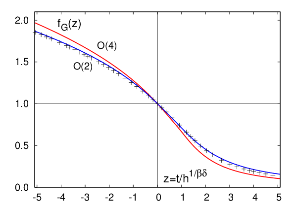

For symmetric spin models in three dimensions the scaling functions have been analyzed in much detail using Monte Carlo simulations and renormalization group techniques. In Fig. 1 we show results for the [13] and [12, 14] scaling functions obtained by using the implicit parametrizations given in Ref. [15] and compiled in Appendix A. There are clear differences between both scaling functions. We note, however, that the manifestation of the differences between the and scaling functions in the limited range shown in Fig. 1 relies also on the normalization of these scaling functions in the limit . Without information on the scaling function at , i.e. in a numerical study that only has access to a limited range of -values, the scale parameters and could easily be adjusted to make the and scaling functions almost coincide. For this is shown by the crosses in Fig. 1 which have been obtained by rescaling the argument of the scaling function, , i.e. through a change of by 20% in this interval. This will lead to a violation of the normalization condition at by a factor , for the scaling function.
The above discussion makes it evident that a numerical analysis of the magnetic equation of state alone, in a scaling regime as large as , will not allow to distinguish scaling from scaling, unless the numerical accuracy is extraordinary high. Additional information will be needed to distinguish from scaling. This can be achieved through accurate control over the chiral limit, , or through the analysis of other scaling functions like the scaling function, , for the susceptibility of the order parameter,
| (6) | |||||
| (7) |
This scaling function is shown in Fig. 1(right). It has a maximum at which together with some critical exponents of the models is given in Table 1. It is obvious from this figure that a simple rescaling of the scale parameter cannot transform an scaling function into that for .
While different symmetric models are characterized by universal scaling functions, the scaling variables have to be normalized properly. The scale parameters and are not universal. They depend on the symmetric model under consideration, the definition of the scaling variables and also on the absolute normalization of the order parameter . For instance, a rescaling of the order parameter by a constant factor, , can be absorbed in a redefinition of the normalization constants and . This leaves the argument of the scaling function and the scaling function itself unchanged, and . For a given definition of the symmetry breaking field the combination therefore remains unchanged and is unique for any symmetric model, i.e. its value is characteristic for that theory. It, for instance, characterizes the -dependence of the pseudo-critical line of transition temperatures, , determined from the peak position of the order parameter susceptibility,
| (8) |
In Section IV we will determine the corresponding scaling relation for the pseudo-critical line of (2+1)-flavor QCD from an analysis of the magnetic equation of state.
| 2 | 0.349 | 1.319 | 4.780 | 0.592(10) | 1.56(10) |
|---|---|---|---|---|---|
| 4 | 0.380 | 1.453 | 4.824 | 0.666(6) | 1.33(5) |
II.2 Contribution of Goldstone modes
The spontaneous breaking of the continuous symmetry at low temperature gives rise to massless Goldstone modes. The fluctuations of these light modes are reflected in the non-analytic dependence of the order parameter on the symmetry breaking variable, [19]. In three dimensions this leads to [19, 21, 22]
| (9) |
This leading correction to the temperature dependence of the order parameter, which arises from a non-vanishing explicit symmetry breaking (), is also reflected in the leading correction to the scaling function . For large, negative values of one has,
| (10) |
As has been discussed also in [15], Eq. 10 can easily be obtained from the magnetic equation of state derived by Wallace and Zia [19]. The universal amplitude is also given in Table 1. In the following we will not make use of the scaling behavior of in the opposite limit, . We note, however, that in this limit is controlled by the critical exponent , . The universal parameter has been determined for three dimensional [23] and [24] universality classes.

The asymptotic form of the scaling function, , gives an excellent approximation to in almost the entire low temperature regime, . This is evident from Fig. 2 where we compare to as well as to the leading order form, . For differences between and are less than 2% for and less than 1% for . The leading -dependent correction that arises from the presence of Goldstone modes thus gives the dominant contribution to the order parameter in this regime. In order to establish universal critical behavior through an analysis of the magnetic equation of state for QCD it therefore will be crucial to establish the influence of the Goldstone mode on the quark mass dependence of the chiral condensate and its derivative, the chiral susceptibility.
III Chiral symmetry breaking in (2+1) flavor QCD
III.1 Quark mass and volume dependence of the chiral condensate
We discuss here our calculations performed for (2+1)-flavor QCD on lattices with size . We have fixed the temporal extent, , and performed calculations for different spatial lattice sizes and to control finite volume effects. All our calculations have been performed with a tree level improved gauge action and an improved staggered fermion action (p4-action), which eliminates discretization errors in thermodynamic observables at the tree level. The value of the bare strange quark mass in lattice units has been fixed to . In earlier calculations of the equation of state [25] and the transition temperature [26], performed with the same improved gauge and staggered fermion actions, it had been shown that in the present (small) range of gauge couplings this value of the strange bare quark mass yields almost physical values for the masses of the strange pseudo-scalar meson and the kaon. The light quark masses have been varied in the range . The smallest value, , corresponds to a pseudo-scalar Goldstone mass of about MeV. For each of the 6 quark mass values chosen in the above interval we have performed calculations at several values of the gauge coupling in the range . As will become clear later this covers a temperature range , with denoting the transition temperature in the chiral limit on a lattice with fixed temporal extent. All calculations have been performed using the Rational Hybrid Monte Carlo (RHMC) algorithm. In most cases we collected 15.000 to 40.000 trajectories with length of half a time unit. We give more details on our simulation parameters, the statistics collected and expectation values of chiral condensates in Appendix B.
Whenever we convert results to physical units we use the scale setting and meson mass calculations performed in connection with our calculation of the equation of state [25] and the transition temperature [26]. The most central anchor point for our current analysis is the determination of the pseudo-scalar mass () and the Sommer scale parameter for light quark masses at a gauge coupling . This value of the gauge coupling is close to the critical temperature in the chiral limit and the light to strange quark mass ratio is close to the physical mass ratio. For this parameter set we find and in lattice units. This converts to MeV when using fm [27] as it has been done also in our earlier calculations.
The main part of our analysis is based on calculations of the light and strange quark chiral condensates,
| (11) |
where and denote the fermion matrices for light and strange quarks, respectively.
A first overview on our data sample is given in the left hand part of Fig. 3. This figure shows results for the light quark chiral condensate in lattice units, calculated for different values of the gauge coupling and 6 different values of the light quark mass. For each parameter set we only show results from the largest spatial lattices available. We comment on finite volume effects below. We also note that we will conclude later that the chiral phase transition temperature at corresponds to . As is evident from Fig. 3 the light quark chiral condensate shows a strong quark mass dependence that is not consistent with a linear dependence on . In fact, at low temperatures the dominant quark mass correction seems to be proportional to . This is highlighted in the right hand part of Fig. 3. Results for the light and strange quark condensates are summarized in Appendix B.


In order to make sure that the drop in , seen for small values of the quark mass, is not due to a too small spatial volume, we analyzed the volume dependence of our results by performing calculations on lattices with spatial extent and . We show some results from this analysis in Fig. 4. As expected, the volume dependence of the chiral condensate increases with decreasing value of the quark mass. We have, however, no evidence for a strong increase of the volume dependence close to the phase transition temperature (). This suggests that also for the smallest quark masses used, our results obtained on lattices of spatial size are close to the infinite volume limit. We also note that the smallest quark mass value used on our largest lattices corresponds to , where denotes the lightest pseudo-scalar meson mass, i.e. the Goldstone meson in the staggered fermion formulation of (2+1)-flavor QCD.


III.2 The chiral order parameter
The chiral condensate, as introduced in Eq. 11, is an order parameter for the chiral phase transition. At non-vanishing light quark mass an additive and multiplicative renormalization is needed to define an order parameter in the continuum limit. In Ref. [25] we introduced an order parameter where quadratically divergent, additive contributions, which are proportional to the quark mass, have been removed by subtracting a suitable fraction of the strange quark chiral condensate from the light quark condensate. We will use this observable also here33 3 This does not remove divergencies that are logarithmic in the cut-off. In the free field limit these divergencies are proportional to and are therefore expected to be numerically small. To take into account the anomalous dimensions of the chiral condensate we introduce a multiplicative renormalization, using the strange quark mass. A similar procedure has been suggested for 2-flavor QCD [5]. Furthermore, we express this product in units of to make it dimensionless. We thus introduce as an order parameter for chiral symmetry restoration in (2+1)-flavor QCD
| (12) |
For our scaling analysis at fixed a renormalization of the order parameter is not at all necessary. We may as well analyze the scaling behavior of the non-subtracted chiral condensate introduced in Eq. 11. To check the consistency of our analysis, we will do so and in the following also utilize the non-subtracted order parameter
| (13) |
where we have introduced the constant multiplicative factor, , such that and agree in the chiral limit.
IV The magnetic equation of state
Having introduced our numerical results for the light and strange quark chiral condensates and the subtracted () and non-subtracted () order parameters, we are now ready to discuss critical behavior in the vicinity of the transition temperature in terms of the magnetic equation of state.
IV.1 Scaling analysis
In the vicinity of the chiral phase transition temperature corresponding to vanishing light quark masses and for sufficiently small explicit symmetry breaking, the order parameter is expected to scale according to Eq. 1. We introduce the reduced temperature and external field variables and as in Eq. 2. The definition of obviously carries over from the spin model context to QCD. For the relation between the lattice gauge coupling and the temperature we exploit the parametrization of the Sommer scale parameter that has been determined in our calculations for the equation of state [25] at . This takes into account deviations from asymptotic scaling of the QCD -function for the range of couplings used here. We checked that the entire scaling analysis presented here only for a small range of the lattice cut-off is not really sensitive to these corrections and could as well have been performed by determining using the asymptotic 2-loop -function or other approaches followed in earlier studies [3, 6, 8]. Likewise this analysis is, of course, independent of any physical value used to set the absolute scale for .
The symmetry breaking external field is proportional to the light quark mass. Also here we take care of the anomalous scaling dimension of quark masses and express the light quark mass in units of the strange quark mass, i.e. we introduce . An alternative, yet similar way to deal with the anomalous dimensions has been suggested in [5].
In the chiral limit, at finite value of the cut-off (fixed ) we expect the phase transition in (2+1)-flavor QCD to be either first order or to belong to the universality class of three dimensional models. In our current analysis we did not find any indication for a strong volume dependence or meta-stabilities in the time evolution of the chiral condensates or other observables. In particular, as is also evident from Fig 10 shown in Section V, we have no evidence for a strong increase in the chiral susceptibility as function of volume. Although we can, at present, not rule out a weak first order phase transition at smaller quark masses, we have no indications for that to happen. We therefore will compare our data on the order parameter to the universal scaling function, i.e. the magnetic equation of state introduced in Eq. 1 with critical exponents and given in Table 1. We start by determining the three free parameters , and the transition temperature, , from fits to the order parameter . For this we use the three lightest quark mass values, , leaving out the lowest temperature value, corresponding to , and the two highest temperature values, corresponding to and . For and these data are from lattices of size while the data set is taken from calculation on lattices.
A posteriori we find that this temperature interval corresponds to . In this small temperature interval and for the small quark mass regime, which does include the light quark mass value corresponding to the physical pion mass, we find good agreement between the rescaled order parameter and the scaling function. This is shown in the left hand part of Fig. 5. The fit yields for the critical coupling corresponding to a phase transition temperature44 4 This value is in excellent agreement with our earlier analysis performed with the p4 action on lattices with temporal extent . We stress, however, that this transition temperature is not extrapolated to the continuum limit and, in fact, within the staggered fermion approach, the chiral extrapolation should be performed after the continuum extrapolation to recover eventually the anticipated scaling behavior. MeV. We obtain an equally good agreement with the scaling curve from an analysis of the non-subtracted order parameter . This is shown in the right hand part of Fig. 5. A similar analysis using the scaling function and critical exponents yields scale parameters that are similar to those of the analysis, the largest differences occurring for which comes out to be about 20% larger.
The scaling function is defined in the limit , , keeping fixed. In this limit the two order parameters and coincide. From our scaling analysis we therefore should find identical results for the scale parameters, i.e. the critical temperature as well as the normalization constants , , if this analysis has been performed sufficiently close to the chiral limit. We have performed the scaling analysis for two different cuts on the ratio of the light to strange quark masses, and . The fit parameters obtained in these two cases from an analysis of data for and are summarized in Table 2. We note that results for and are within errors independent on the cut on and the observable used. The scale parameter is more sensitive on the choice of order parameter. However, there is a tendency that results for obtained from and converge to a common value if the cut on is reduced.
| [MeV] | |||||
|---|---|---|---|---|---|
| 1/20 | 0.0048(5) | 0.0048(2) | 195.6(4) | 8.5 (7) | |
| 1/20 | 0.0022(3) | 0.0037(2) | 194.5(4) | 6.8 (5) | |
| 1/40 | 0.0042(6) | 0.0047(2) | 195.3(4) | 8.0 (8) | |
| 1/40 | 0.0025(5) | 0.0040(2) | 194.8(4) | 7.0 (6) |
The symmetry breaking field introduced in Eq. 2 is given in terms of the ratio of light to strange quark masses. To compare our result for scaling functions of QCD with other (model) calculations it may be more convenient to express in terms of meson masses. In the present quark mass and gauge coupling range we find the approximate relation . We therefore may write the scaling variable as
| (14) |
As discussed in Section II this allows to determine the scaling behavior of the pseudo-critical line determined by the peak in the scaling function of the chiral susceptibility, ,
| (15) |
Using from Table 1 and the values for given in Table 2 we find . These values, which are consistent with earlier determinations of the slope of the pseudo-critical line [26, 28], emphasizes the weak dependence of the pseudo-critical temperature on the pseudo-scalar meson mass.
We stress that this analysis has been performed in QCD at one non-vanishing lattice spacing, i.e. in the cut-off theory. The cut-off dependence of the normalization constants, the scale invariant ratio and the subtle continuum limit need to be studied in the future. We emphasize again, however, that the above combination of normalization constants for the scaling variables is an invariant of QCD and depends, in the continuum limit, only on the strange quark mass value.


IV.2 Scaling violations


The scaling behavior observed for the chiral order parameters analyzed in the previous section is, of course, expected to hold exactly only in the limit and , keeping the ratio fixed. At non-zero values of and we expect to observe scaling violations that may arise from sub-leading corrections to the scaling function as well as from the regular part of the QCD partition function. These corrections also depend on the definition of the order parameter. In particular, the two order parameters, and , introduced here differ in the treatment of contributions that are linear in the light quark mass. In our analysis of the order parameter, performed in a larger temperature and quark mass interval, we clearly see these differences and their role in contributing to violations of scaling. This is shown in Fig. 6. Most prominent are effects arising from a too large quark mass value. These effects show up in the scaling plot as deviations from the scaling function in the region of small , i.e. for large quark masses at fixed . They lead to the sizeable displacement of results obtained for too heavy quarks from the scaling curve. Effects that arise because the temperatures chosen are too far away from the critical point, , are typically not that drastic in our data sample. We fitted the scaling violations to an ansatz
| (16) |
We also considered including a term quadratic in the reduced temperature (). This correction, however, turned out to vanish within the errors of our fits.
The fits of both order parameters performed with the ansatz given in Eq. 16 are shown in Fig. 7. As expected, we find that corrections linear in are eliminated in . The corresponding fit parameter is zero within errors and we therefore have fixed it to be zero in the fit shown in Fig. 7 (left). For the non-subtracted order parameter this term gives the dominant finite quark mass corrections. Here we find .


IV.3 Scaling of the chiral condensate
We have seen in the previous section that order parameters constructed from the chiral condensate are well described by the magnetic equation of state for small enough values of the light quark masses, . We want to underscore this point here by displaying the order parameters not in their scaling form, but as a function of temperature in units of the transition temperature determined in the previous section. This is shown in Fig. 8. The curves drawn in this figure are taken from the scaling fits to the subtracted and non-subtracted order parameters shown in Fig. 5. They had been obtained from the numerical results for (left) and (right) in the range and .


IV.4 Comparison with earlier calculations in 2-flavor QCD
As mentioned in the Introduction, there have been earlier attempts to compare the quark mass and temperature dependence of the chiral order parameter with scaling functions on lattices with temporal extent [6, 8, 9]. These calculations had been performed for 2-flavor QCD using unimproved gauge and staggered fermion actions. In Ref. [6] calculations with three quark mass values had been performed, and . The last two masses are similar to the two mass values used in Ref. [8], i.e. and . In fact, results for chiral condensates obtained in these two calculations are in good agreement with each other. This also is true for calculations performed in [4] where has been used. All these calculations have been performed at values of the gauge coupling in the vicinity of the cross-over at the corresponding quark mass values. They therefore mostly explored the region of .
In Fig. 9 we compare results for the chiral condensate obtained in 2-flavor calculations with unimproved gauge and fermion actions with our results obtained in (2+1)-flavor QCD with improved gauge and fermion actions. In this figure we use a log-log plot as has been done also in Ref. [6]. In the 2-flavor case the symmetry breaking field has usually been chosen as while for the reduced temperature variable we used , with as estimate for the critical value of the gauge coupling in the chiral limit [8] and ) denoting the 2-loop -function for 2-flavor QCD. In the log-log plot differences in the scale parameters and correspond to shifts in vertical and horizontal directions, respectively. We made no effort to optimize the choice of these scale parameters for the 2-flavor data set. In Fig. 9 we have positioned the data such that the crossover region roughly corresponds to the location of the maximum in the scaling function , with (see also [9]); this required the choice .
When comparing results obtained with standard and improved gauge actions the difference in the shape of the data sets clearly is the most striking feature. Apparently the (2+1)-flavor data set is in good agreement with scaling while the results obtained with the standard staggered action deviate strongly. Furthermore, there is no tendency for better agreement with decreasing quark mass. Closer to the continuum limit, i.e. for larger , results obtained with the unimproved actions have a similar shape [6] but seem to get somewhat closer to the scaling curve.
To compare the quark mass values used in the 2-flavor QCD calculations with those of the present (2+1)-flavor study we note that for standard staggered fermions at gauge couplings close to the cross-over a bare quark mass corresponds to a pseudo-scalar Goldstone mass MeV [30]. The lightest quark mass used in these calculations, , therefore corresponds to MeV, which is similar to the pseudo-scalar mass obtained in (2+1)-flavor QCD calculations for the light to strange quark mass ratio . At this value for the light quark mass we observe only mild violations of scaling in calculations with the improved gauge and fermion actions.
The number of flavors as well as the quark masses are different in the data sets compared in Fig. 9. Nevertheless, it seems unlikely that this is the origin of the observed differences. It appears more probable that cut-off effects in calculations with unimproved gauge and fermion actions cause the differences.

V Susceptibilities
In Eq. 6 we introduced the susceptibility as the derivative of the order parameter with respect to the symmetry breaking field. Its temperature and quark mass dependence is controlled by the scaling function defined in Eq. 7, which is shown in the right hand part of Fig. 1 for and . Similarly we can, of course, introduce the susceptibility as a derivative of the order parameter with respect to . Taking derivatives with respect to , rather than with respect to the ratio of quark masses, , obviously requires knowledge of the scale parameter which we have determined in the previous section.
In the analysis of QCD thermodynamics on the lattice it is more customary to calculate light () and strange () quark chiral susceptibilities, which are defined as derivatives of the corresponding chiral condensates with respect to and , respectively
| (17) |
To construct the susceptibility we will also need to take into account a mixed chiral susceptibility,
| (19) |
The susceptibility of the subtracted order parameter, , is then obtained as
| (20) | |||||
where in the last equality we introduced the susceptibility , of the non-subtracted order parameter . With this we can construct the scaling function for the chiral susceptibility,
| (21) |
from and similarly also from .
The scaling functions , constructed from either or , differ by terms that vanish in the chiral limit at . These terms therefore characterize once more systematic differences that arise in the construction of scaling functions due to the presence of regular terms that vanish, once the appropriate scaling limits are taken. We show scaling functions constructed from both order parameters in Fig. 10. We stress that all parameters (, and ) have been determined in our analysis of the order parameters themselves. No fits are therefore involved in the comparison of the scaling functions with the numerical results for susceptibilities shown in this figure.
It is obvious from Fig. 10 that violations of scaling are significantly larger for susceptibilities than for the order parameters. Susceptibilities extracted from and still differ for but start to become compatible within errors for . For we also show results from calculations on two different lattice size, and . If any, the volume dependence of susceptibilities is small at this value of the quark mass.
There is yet another difference between order parameter susceptibilities derived in QCD, where the order parameter is a composed operator constructed from fermionic fields, and spin models, where the order parameter is the expectation value of a scalar boson field. The order parameter susceptibilities in QCD receive two contributions, usually called the disconnected and connected part of the susceptibility,
| (22) |
with
| (23) | |||||
| (24) |
While the first term, the disconnected part of the light quark susceptibility, describes fluctuations of the light quark condensate and has a direct analogy in the fluctuations of the order parameter in an spin model, the second term () arises from the explicit quark mass dependence of the order parameter, the chiral condensate. The connected part is an integral over the (quark-line connected) correlation function of the (iso-vector) scalar operator, . The integral has a rather subtle quark mass dependence. Since , however, will vanish in the chiral limit. In this limit the connected part of the susceptibility will therefore not contribute to the scaling function which in turn will entirely be determined through the disconnected part of the light quark susceptibility.
At non-vanishing values of the light quark mass, however, the non-vanishing connected part of the chiral susceptibility is responsible for additional scaling violations in . In fact, the scaling violations due to the connected part are distinctively different between and symmetric theories [22]. It is only in the latter that fluctuations of Goldstone modes do not contribute to . In the case of symmetric models is expected to diverge proportional to just like the total order parameter susceptibilities will do.
In the staggered formulation of QCD with 2 light quark flavors the lack of symmetry in the Lagrangian is due to explicit symmetry breaking terms (taste violations) that disappear only in the continuum limit. Corresponding to the spin models, at finite values of the cut-off the divergence of in the chiral limit can thus be understood in terms of taste violating contributions to the scalar correlation function [31]. We will discuss these subtle aspects of susceptibilities of the order parameter, the influence of taste violating terms in the staggered action on scaling properties of these susceptibilities and the resulting cut-off dependence of in more detail in a forthcoming publication [32].


VI Conclusions
We have performed a new analysis of scaling properties of the light quark chiral condensate in -flavor QCD. We found that at fixed non-zero lattice spacing the chiral condensate calculated with improved staggered fermions shows scaling behavior in the chiral limit that is consistent with scaling.
Through the analysis of scaling properties with quark masses that are smaller than the physical light quark masses we could fix the normalization constants and in the scaling variables and . This allowed us to quantify scaling violations for non-zero values of the quark masses in the vicinity of the phase transition temperature. These scaling violations turned out to be small in the magnetic equation of state already for physical values of the quark mass.
On the basis of studying just the magnetic equation of state, we gave arguments that it will remain difficult to rule out scaling without extraordinary precision of numerical lattice data. However, a distinction between and scaling might become possible through an accurate analysis of susceptibilities of the order parameter. At present, we still find significant deviations from scaling for the chiral susceptibility. This will be discussed in more detail in a forthcoming publication [32].
A determination of and also fixes the scale parameter , which controls the quark mass dependence of the pseudo-critical line determined from the peak in the chiral susceptibility. In our present analysis this parameter, which uniquely characterizes non-universal aspects of critical behavior in QCD, has only been determined at one value of the lattice cut-off. Calculations at smaller lattice spacings, together with good control over scaling violations induced at non-vanishing quark masses will be needed to extract in the symmetric continuum limit.
The good scaling properties found here in calculations with improved gauge and fermion actions are in contrast to earlier calculations that had been performed with unimproved staggered fermion and gauge actions. We argued that the observed differences are due to cut-off effects.
In our analysis we have assumed that the strange quark mass in -flavor QCD is large enough to avoid a first order phase transition in the light quark chiral limit. Although the good scaling properties of the chiral order parameters and the absence of a strong volume dependence in the light quark susceptibilities support this assumption, we clearly cannot exclude a first order transition to occur at still lighter quark masses. Consistent with limits given on the location of a first order transition in 3-flavor QCD [33, 34], however, our current analysis rules out such a transition for pseudo-scalar masses MeV.
Acknowledgments
This work has been supported in part by contracts DE-AC02-98CH10886 with the U.S. Department of Energy, the BMBF under grant 06BI401, the Gesellschaft für Schwerionenforschung under grant BILAER, the Extreme Matter Institute under grant HA216/EMMI and the Deutsche Forschungsgemeinschaft under grant GRK 881. Numerical simulations have been performed on the BlueGene/L at the New York Center for Computational Sciences (NYCCS) which is supported by the U.S. Department of Energy and by the State of New York as well as the QCDOC computer of USQCD. We thank J. Engels for discussions and for providing us with his programs to calculate the scaling functions.
Appendix A Scaling functions for three-dimensional and models
In this appendix we summarize the scaling functions for models in the three-dimensional and universality classes. These interpolating functions have been taken from Ref. [15] and [16]. We note that the original parameters for the model published in the tables of Ref. [15] had been updated in [16]. Moreover, interpolating curves had been constructed only for the scaling function . Applying these interpolations also to required slight adjustments of the interpolation parameters (, ).
In Eq. 1 we expressed the dependence of the order parameter on the scaling variables and in terms of a scaling function, . Following the discussion given in [15] we introduce the variables and ,
| (25) |
Obviously . For small and large values of the asymptotic forms that relate to are known. For small we have
| (26) |
and for large values of one finds
| (27) |
One can smoothly interpolate between these two relations [15] using the ansatz
| (28) |
This ansatz has been used to obtain the scaling functions shown in Fig. 1 for . For outside this interval the asymptotic expressions and have been used. The constant and the critical exponents are given in Table 1, the other parameters needed for this interpolation are collected in Table 3.
| 0.352(30) | 0.056 | 1.260(3) | -1.163(20) | 2.5 | 3 | |
| 0.359(10) | -0.025(10) | 1.071(4) | -0.866(38) | 5.0 | 3 |
Appendix B Chiral condensates from calculations on lattices with temporal extent
In this appendix we present data of our calculations performed with the p4 staggered fermion action on lattices with temporal extent and spatial extent , and . All calculations have been performed with 2 light quarks and a strange quark of mass . The improved gauge and fermion actions used for these calculations have been described in detail in Ref. [35]. The tables give results of calculations performed at different values of the gauge coupling (). Results for light () and strange () quark condensates as well as the disconnected and connected contributions to the corresponding susceptibilities are normalized to a single flavor. The last column gives the number of trajectories generated for each parameter set.
In Table 6 we give for some selected values of the gauge coupling the conversion to a reduced temperature scale.
| # traj. | |||||||
| , | |||||||
| 3.2800 | 0.1322(3) | 3.90(16) | 2.43(24) | 0.2575(1) | 1.412(1) | 0.47(4) | 18730 |
| 3.2900 | 0.1082(4) | 4.73(12) | 3.95(34) | 0.2454(1) | 1.477(1) | 0.63(5) | 20070 |
| 3.3000 | 0.0715(4) | 7.44(11) | 6.10(44) | 0.2294(1) | 1.575(1) | 0.63(4) | 18830 |
| 3.3025 | 0.0633(6) | 8.46(13) | 7.61(67) | 0.2261(2) | 1.593(1) | 0.77(7) | 15810 |
| 3.3050 | 0.0553(5) | 9.44(12) | 7.46(55) | 0.2228(2) | 1.613(1) | 0.78(7) | 17460 |
| 3.3075 | 0.0459(15) | 11.30(35) | 9.91(1.47) | 0.2190(5) | 1.634(3) | 1.04(17) | 4530 |
| 3.3100 | 0.0376(5) | 12.31(14) | 6.85(53) | 0.2156(1) | 1.656(1) | 0.70(6) | 15850 |
| 3.3200 | 0.0195(4) | 12.98(17) | 3.07(23) | 0.2054(2) | 1.706(2) | 0.57(4) | 10380 |
| 3.3300 | 0.0111(2) | 10.48(11) | 0.88(10) | 0.1968(1) | 1.745(1) | 0.40(4) | 6850 |
| , | |||||||
| 3.2800 | 0.1386(2) | 3.15(5) | 1.81(14) | 0.2590(1) | 1.400(1) | 0.42(3) | 21080 |
| 3.2850 | 0.1290(8) | 3.28(20) | 2.48(73) | 0.2536(3) | 1.433(3) | 0.51(13) | 3400 |
| 3.2900 | 0.1181(3) | 3.80(6) | 3.36(26) | 0.2479(1) | 1.460(1) | 0.62(5) | 20940 |
| 3.2950 | 0.1009(12) | 4.41(20) | 2.28(49) | 0.2396(5) | 1.505(4) | 0.41(6) | 1900 |
| 3.3000 | 0.0888(4) | 5.10(6) | 4.95(39) | 0.2336(1) | 1.543(1) | 0.74(6) | 20550 |
| 3.3025 | 0.0797(5) | 5.63(8) | 6.04(57) | 0.2295(2) | 1.568(2) | 0.89(9) | 16870 |
| 3.3050 | 0.0690(4) | 6.47(6) | 5.17(35) | 0.2249(1) | 1.599(1) | 0.69(5) | 21280 |
| 3.3075 | 0.0621(7) | 6.94(9) | 4.98(45) | 0.2217(2) | 1.616(2) | 0.63(6) | 6570 |
| 3.3100 | 0.0545(7) | 7.45(9) | 4.74(78) | 0.2183(3) | 1.633(2) | 0.72(14) | 7370 |
| , | |||||||
| 3.2800 | 0.1380(7) | 3.77(12) | 2.12(13) | 0.2593(3) | 1.401(2) | 0.44(3) | 21180 |
| 3.2900 | 0.1165(7) | 4.47(12) | 3.10(17) | 0.2475(3) | 1.462(2) | 0.55(3) | 27440 |
| 3.3000 | 0.0880(10) | 5.74(11) | 5.35(38) | 0.2337(4) | 1.541(3) | 0.76(6) | 40000 |
| 3.3050 | 0.0688(10) | 7.11(10) | 5.83(40) | 0.2252(4) | 1.599(3) | 0.82(7) | 42000 |
| 3.3100 | 0.0533(11) | 8.14(13) | 4.88(30) | 0.2182(4) | 1.636(3) | 0.63(4) | 24910 |
| 3.3200 | 0.0334(7) | 9.05(8) | 2.95(14) | 0.2075(3) | 1.692(2) | 0.51(3) | 25050 |
| 3.3300 | 0.0202(4) | 8.16(9) | 1.09(6) | 0.1975(3) | 1.740(2) | 0.39(3) | 14870 |
| , | |||||||
| 3.2800 | 0.1487(4) | 2.84(8) | 1.73(8) | 0.2615(2) | 1.374(3) | 0.44(2) | 40360 |
| 3.2850 | 0.1421(9) | 2.93(10) | 1.98(20) | 0.2575(5) | 1.405(5) | 0.49(5) | 13260 |
| 3.2900 | 0.1308(5) | 3.20(3) | 2.20(11) | 0.2510(2) | 1.433(2) | 0.50(2) | 45080 |
| 3.2950 | 0.1204(9) | 3.56(7) | 2.69(17) | 0.2454(4) | 1.469(4) | 0.60(4) | 19110 |
| 3.3000 | 0.1083(6) | 3.88(3) | 3.16(18) | 0.2388(3) | 1.504(2) | 0.64(3) | 41050 |
| 3.3050 | 0.0933(7) | 4.43(5) | 3.97(21) | 0.2312(3) | 1.551(3) | 0.76(4) | 39960 |
| 3.3100 | 0.0792(7) | 4.82(5) | 4.12(18) | 0.2239(3) | 1.586(3) | 0.77(3) | 42890 |
| 3.3200 | 0.0542(6) | 5.88(4) | 3.16(14) | 0.2107(2) | 1.668(2) | 0.66(3) | 44490 |
| 3.3300 | 0.0336(3) | 6.25(2) | 1.41(8) | 0.1984(2) | 1.734(1) | 0.46(2) | 39320 |
| , | |||||||
| 3.2800 | 0.1488(2) | - | 1.61(13) | 0.2615(1) | - | 0.46(3) | 20000 |
| , | |||||||
| 3.3000 | 0.0627(25) | - | 7.64(94) | 0.2279(9) | - | 0.71(10) | 6690 |
| , | |||||||
| 3.3000 | 0.0452(21) | - | 4.68(39) | 0.2335(13) | - | 0.70(5) | 25830 |
| , | |||||||
| 3.2800 | 0.1141(29) | - | 5.26(25) | 0.2584(12) | - | 0.51(4) | 38280 |
| 3.2900 | 0.0963(21) | - | 5.24(17) | 0.2485(9) | - | 0.61(3) | 40660 |
| 3.3000 | 0.0753(35) | - | 5.32(34) | 0.2380(16) | - | 0.75(6) | 40100 |
| , | |||||||
| 3.3000 | 0.0954(21) | - | 3.49(13) | 0.2372(10) | - | 0.63(3) | 30000 |
| # traj. | |||||||
| , | |||||||
| 3.2800 | 0.1660(4) | 2.37(1) | 1.11(6) | 0.2661(2) | 1.352(1) | 0.37(2) | 27550 |
| 3.2850 | 0.1595(5) | 2.50(2) | 1.14(8) | 0.2619(2) | 1.371(2) | 0.38(2) | 19150 |
| 3.2900 | 0.1507(4) | 2.60(1) | 1.37(7) | 0.2562(2) | 1.402(2) | 0.43(2) | 30160 |
| 3.2950 | 0.1439(5) | 2.74(2) | 1.77(12) | 0.2519(3) | 1.424(2) | 0.53(3) | 24880 |
| 3.3000 | 0.1351(5) | 2.85(1) | 1.94(12) | 0.2464(2) | 1.452(2) | 0.57(3) | 36100 |
| 3.3050 | 0.1269(5) | 3.01(4) | 2.23(12) | 0.2414(3) | 1.471(5) | 0.63(3) | 40230 |
| 3.3100 | 0.1146(6) | 3.22(4) | 2.74(15) | 0.2343(3) | 1.515(5) | 0.74(4) | 40440 |
| 3.3150 | 0.1007(6) | 3.53(3) | 3.09(15) | 0.2262(3) | 1.555(4) | 0.81(4) | 45570 |
| 3.3200 | 0.0895(6) | 3.80(2) | 2.53(15) | 0.2197(3) | 1.597(3) | 0.65(4) | 33360 |
| 3.3300 | 0.0666(8) | 4.29(2) | 2.10(14) | 0.2061(4) | 1.678(3) | 0.62(4) | 18060 |
| , | |||||||
| 3.2800 | 0.1899(3) | 1.98(0) | 0.59(3) | 0.2722(2) | 1.317(1) | 0.28(1) | 20050 |
| 3.2900 | 0.1795(4) | 2.07(0) | 0.79(4) | 0.2645(2) | 1.350(1) | 0.34(1) | 21040 |
| 3.3000 | 0.1687(5) | 2.18(1) | 1.06(7) | 0.2565(3) | 1.387(3) | 0.45(3) | 18880 |
| 3.3050 | 0.1621(4) | 2.27(1) | 1.03(6) | 0.2518(2) | 1.413(4) | 0.43(2) | 32170 |
| 3.3100 | 0.1555(6) | 2.31(1) | 1.05(9) | 0.2470(4) | 1.429(2) | 0.44(3) | 16580 |
| 3.3200 | 0.1383(6) | 2.55(2) | 1.67(10) | 0.2354(3) | 1.492(4) | 0.64(4) | 28740 |
| 3.3250 | 0.1295(4) | 2.72(3) | 1.81(9) | 0.2295(2) | 1.530(13) | 0.68(3) | 54840 |
| 3.3300 | 0.1186(5) | 2.81(1) | 1.92(9) | 0.2222(3) | 1.566(2) | 0.72(3) | 50000 |
| , | |||||||
| 3.2800 | 0.2256(2) | 1.62(0) | 0.39(2) | 0.2812(1) | 1.267(1) | 0.24(1) | 20310 |
| 3.2900 | 0.2180(2) | 1.66(0) | 0.42(2) | 0.2747(2) | 1.290(1) | 0.25(1) | 23950 |
| 3.3000 | 0.2105(3) | 1.71(0) | 0.45(2) | 0.2683(2) | 1.314(2) | 0.27(1) | 15330 |
| 3.3050 | 0.2054(3) | 1.73(0) | 0.44(3) | 0.2642(2) | 1.331(1) | 0.27(1) | 22550 |
| 3.3100 | 0.2010(3) | 1.76(1) | 0.57(4) | 0.2605(2) | 1.346(4) | 0.34(2) | 20170 |
| 3.3200 | 0.1916(4) | 1.82(0) | 0.67(4) | 0.2528(3) | 1.378(1) | 0.39(2) | 20030 |
| 3.3300 | 0.1807(4) | 1.90(0) | 0.74(6) | 0.2440(3) | 1.417(2) | 0.41(3) | 23380 |
| 3.2800 | 3.2900 | 3.3000 | 3.3100 | 3.3200 | 3.3300 | |
| -0.0332 | -0.0170 | 0.0000 | 0.0181 | 0.0379 | 0.0595 |
References
- [1] R. Pisarski and F. Wilczek, Phys. Rev. D 29, 338 (1984).
- [2] see for instance, S. Gupta, J. Phys. G 35, 104018 (2008).
- [3] F. Karsch, Phys. Rev. D 49, 3791 (1994).
- [4]
F. Karsch and E. Laermann,
Phys. Rev. D 50, 6954 (1994);
E. Laermann, Nucl. Phys. Proc. Suppl. 60A, 180, 1998. - [5] C. W. Bernard et al., Phys. Rev. D 54, 4585 (1996).
- [6] C. W. Bernard et al., Phys. Rev. D 61, 054503 (2000).
- [7] S. Aoki et al. (JLQCD Collaboration), Phys. Rev. D 57, 3910 (1998).
- [8] M. D’Elia, A. Di Giacomo and C. Pica, Phys. Rev. D 72, 114510 (2005).
- [9] T. Mendes, PoS LAT2007, 208 (2007).
- [10] Y. Iwasaki, K. Kanaya, S. Kaya and T. Yoshíe, Phys. Rev. Lett. 78, 179 (1997).
- [11] A. Ali Khan et al. (CP-PACS Collaboration), Phys. Rev. D 63, 034502 (2001).
- [12] D. Toussaint, Phys. Rev. D 55, 362 (1997).
- [13] J. Engels, S. Holtmann, T. Mendes and T. Schulze, Phys. Lett. B 492, 219 (2000).
- [14] J. Engels and T. Mendes, Nucl. Phys. B 572, 289 (2000).
- [15] J. Engels, S. Holtmann, T. Mendes and T. Schulze, Phys. Lett. B 514, 299 (2001).
- [16] J. Engels, L. Fromme and M. Seniuch, Nucl. Phys. B 675 [FS], 533 (2003).
- [17] J. B. Kogut and D. K. Sinclair, Phys. Rev. D 73, 074512 (2006).
- [18] J. Engels, S. Holtmann and T. Schulze, PoS LAT2005, 148 (2005).
- [19] D.J. Wallace and R.K.P. Zia, Phys. Rev. B 12, 5340 (1975).
- [20] J. Gasser and H. Leutwyler, Phys. Lett. B 184, 83 (1987).
- [21] P. Hasenfratz and H. Leutwyler, Nucl. Phys. B 343, 241 (1990),
- [22]
A. V. Smilga, Phys. Lett. B 318, 531 (1993);
A. V. Smilga and J. J. M. Verbaarschot, Phys. Rev. D 54, 1087 (1996). - [23] M. Campostrini, M. Hasenbusch, A. Pelissetto, P. Rossi and E. Vicari, Phys. Rev. B 63, 214503 (2001).
- [24] A. Butti, F. Parisen Toldin, A. Pelissetto and E. Vicari, Nucl. Phys. Proc. Suppl. 140, 808 (2005).
- [25] M. Cheng et al. (RBC-Bielefeld Collaboration), Phys. Rev. D 77, 014511 (2008).
- [26] M. Cheng et al. (RBC-Bielefeld Collaboration), Phys. Rev. D 74, 054507 (2006).
- [27] M. Gray et al., Phys. Rev. D 72, 094507 (2005).
- [28] F. Karsch, E. Laermann and A. Peikert, Nucl. Phys. B 605, 579 (2001).
- [29] C. Bernard et al. (MILC Collaboration), Phys. Rev. D 71, 034504 (2005).
- [30]
T. Blum, L. Kärkkäinen, D. Toussaint and S. Gottlieb,
Phys. Rev. D 51, 5153 (1995);
C. Bernard et al. (MILC Collaboration), Phys. Rev. D 56, 5584 (1997). - [31] C. Bernard, C. DeTar, Z. Fu and S. Prelovsek, Phys. Rev. D 76, 094504 (2007).
- [32] W. Unger et al., in preparation.
- [33] C. Schmidt et al., Nucl. Phys. Proc. Suppl. 119, 517 (2003).
- [34] G. Endrodi, Z. Fodor, S.D. Katz and K.K. Szabo, PoS LAT2007, 182 (2007).
- [35] F. Karsch, E. Laermann and A. Peikert, Phys. Lett. B 478, 447 (2000).