Reconstruction of the Primordial Power Spectrum by Direct Inversion
Abstract
We introduce a new method for reconstructing the primordial power spectrum, , directly from observations of the Cosmic Microwave Background (CMB). We employ Singular Value Decomposition (SVD) to invert the radiation perturbation transfer function. The degeneracy of the multipole to wavenumber linear mapping is thus reduced. This enables the inversion to be carried out at each point along a Monte Carlo Markov Chain (MCMC) exploration of the combined and cosmological parameter space. We present best–fit obtained with this method along with other cosmological parameters.
Keywords:
Primordial Power Spectrum, CMB, InversionI Introduction
The primordial power spectrum of scalar, curvature perturbations is defined as,
| (1) |
where is the wavenumber. The spectrum encodes the initial conditions for the system of coupled Einstein–Boltzmann equations which describe the evolution of density and radiation perturbations about the FRW background. The spectrum itself is considered as a unique window into the era approaching the Planck time. In most models a period of scalar field driven inflation is used to solve the cosmological problems and set the near scale-invariant form of prior to the radiation dominated epoch. In this case a simple power law parametrised by an amplitude and spectral index suffices to describe the initial conditions to sufficient accuracy for the current data. Higher order contributions such as a mild curvature have also been explored although it is not strictly required by the best–fit models.
A separate approach to studying the physics behind this early phase is to drop any model dependent assumptions of near scale invariance and allow more general functional forms of the initial spectrum. One drawback of this approach is the increase in parameter space which needs to be explored which increases the complexity of the data fitting step. A second drawback is the limited information content of the observations; the effect of sample variance, limited range of scales probed, and the degeneracy in the mapping of to angular multipoles on the sky means that one cannot expect to constrain arbitrarily complex functions with many degrees of freedom. However there is scope to go beyond the model dependent approach. This is particularly true if one is interested in constraining the presence of features on the spectrum. These could be in the form of ‘glitches’ or step–like features which would be otherwise unconstrained. In fact many models have been proposed which predict features on the spectrum due to, for example, features on the inflaton potential [1, 2, 3, 4, 5, 6, 7, 8], a small number of -folds [9, 10, 11], or other more exotic sources of non-standard behaviour [12, 13, 14, 15, 16].
There are two approaches to reconstructing ; parameterisation and direct inversion. None of the various methods have shown conclusive evidence for a departure from near scale-invariance of . Despite this there have been tantalising hints of anomalous features in the CMB. One example of this is that the first year WMAP results gave an indication of a cut-off in on large scales. With subsequent data releases the significance of this feature has been reduced, although future observations of the polarisation of the CMB may provide more conclusive evidence [11, 17]. In [18] we also showed evidence for a dip in power at Mpc-1.
Numerous parametertic searches for features with a similar form to those in complex inflationary models have been performed along with simple binning of [19, 9, 20, 21, 22, 23, 24, 25, 26, 27, 28]. Methods of direct inversion which make no assumptions about the early universe model being probed [29, 30, 31, 32, 19, 33, 34, 35, 36, 37, 38, 39, 40, 41, 42, 43, 18] are hampered by the singular nature of the transfer function that takes and transfers it onto the CMB or LSS modes. In general this causes the process of estimation to be prohibitively slow so as not to allow joint estimation of a free with cosmological parameters. Instead one usually assumes a set of cosmological parameters, this allows the use of a fiducial CMB photon transfer function to integrate the primordial curvature perturbation into today’s photon distribution perturbation. However, this hides a significant degeneracy between features in the primordial power spectrum, and the physical parameters which determine the height and position of acoustic peaks in the CMB. It has been pointed out [44, 18, 45] that adding polarisation information or LSS data can help break some of the degeneracies.
In this paper we propose a new method for direct inversion of from CMB observation using Singular Value Decomposition (SVD). The method is fast enough to allow us to carry out a joint estimation of and the cosmological parameters. The form of is derived from the SVD inversion. We also show that there are regions of for which polarisation data has the potential to more accurately constrain . The paper is organised as follows; in section II we introduce the SVD method and test it against known input models in section III. We also show current constraints from the joint estimation of cosmological parameters and reconstructions in section IV. We discuss our results and conclude in section V.
II Direct Inversion of by Singular Value Decomposition
Direct primordial power spectrum reconstruction requires the inversion of the following relations
| (2) |
where and represent , , or -type anisotropies, are the angular power spectra for the combination and the are the photon perturbation transfer functions. The transfer functions are obtained by integrating the full Einstein-Boltzmann system of differential equations [46, 47]. These describe the evolution of perturbations in the photon distribution functions in the presence of gravity and other sources of stress-energy. The functions determine all of the structure in the anisotropy spectra which arise after the initial conditions are set. Most notably the contain distinct peaks due to the acoustic oscillation of the tightly coupled photon-baryon fluid in gravitational potential wells at the time of last scattering. The aim of any inversion method is to distinguish such features from any structure in the initial perturbation spectrum.
For a finite sampling of the wavenumber space Eq. (2) can be recast as an operator acting on the primordial spectrum
| (3) |
with operator
| (4) |
where are the logarithmic intervals for the discrete sampling chosen in the integration of the system of equations.
A solution for cannot be obtained from a direct inversion of the as it is numerically singular. This is due to the high level of degeneracy in the transfer functions relating the power at any wavenumber to angular multipoles . We instead approximate the inversion by using the SVD method, first reducing the degeneracy of the system and then inverting using the remaining orthogonal modes.
The transfer functions can be factorised as
| (5) |
where the matrices and are unitary and of dimensions and respectively, and is a non-negative, diagonal matrix with diagonal elements . For this application, the dimensions of the matrices are that i.e. there are more equations than modes of interest. This results in some of the diagonal elements of being singular (numerically zero) which prevent the inversion of the transfer matrix.
The SVD method allows one to invert such a system by nulling the singular modes. This is achieved by creating an inverse where the diagonal elements are except where the value of is singular in which case it is replaced by .
In practice we rank order the factorised modes in descending order of and all modes with condition number less than a threshold are nulled, for this work. Thus the method is a ‘-to-’ compression of the system where we keep the least degenerate modes connecting the 3d Fourier space to the 2d angular multipole space. This is not to be confused with a signal-to-noise compression of the data which aims to select with respect to orthogonal modes of the covariance of the observations [48].
It is instructive to look at the first few orthogonal modes given by the columns of the matrix. We plot the first six in Fig. 1. These -space modes are the least degenerate (or best determined) in the mapping provided by the CMB physics. In other words, in the absence of sample and noise variance, these modes pick out the -range where observing the CMB will have the highest impact upon the reconstructed . Not surprisingly, the first few modes are peaked around the angular scales where the acoustic signal from each polarisation combination is maximised. As these are the best constrained vectors in space in the absence of all errors, they are not necessarily the basis vectors of which are most accurately constrained, [44] show what they are for WMAP. We assume that this ordering of singular values is the optimal method for sorting the columns in and .

Once has been computed the primordial power spectrum can be reconstructed by inverting a set of observed using
| (6) | |||||
Our choice of is a conservative one with approximately 200 non-singular modes for a typical transfer matrix. Reconstructing the primordial power spectrum in this way means that we are not using any degenerate modes which carry no information in space but can increase the scatter in the reconstructed spectrum. However we are still susceptible to the scatter in the observed since we have not used any noise weighting in this scheme.
In practice we start our inversion process with a guess input spectrum, parameterised by the usual form . From this and our fiducial cosmological model we obtain a spectrum. We use this to calculate the residual spectrum,
| (7) |
so as to minimise the error induced in -space by the cut-offs in , both on large and small scales.
To remove high frequency oscillations in the data we apply a low-pass filter to the resultant . The following algorithm was used,
| (8) |
where was taken to be . This method of smoothing leaves the first few points in the series strongly influenced by . Therefore one should take any effects seen at low with a pinch of salt as these points are highly correlated. The covariance matrix was altered appropriately by a lower-triangular matrix representing this filter.
We then proceed to bin the reconstructed power spectrum using the optimal binning method of [49]. This binning method estimates a series of ranges in over which the signal-to-noise in the measured primordial power spectrum is constant. Many of the data points are highly correlated with their nearest neighbours and optimal binning gives a clear indication of the scales on which we have independent information. The centre of the bins chosen by the cosmological tool CAMB [47] change when the input cosmological parameters are altered. This is a problem when it is run over many realisations as in the case of a Markov Chain. We choose the optimal binning method to find the standardised output of centres and sizes of bins for each call of the CAMB routine.
To find the optimal binning of the reconstructed power spectrum we investigate how the uncertainty in the transfers into uncertainty in the primordial power spectrum. For this purpose, we need to define the primordial power spectrum as a series of top-hat bins:
| (9) |
where is the power in each bin and if and otherwise. To obtain the errors for these bins we define the Fisher matrix for the by
| (10) |
where is the diagonal matrix of the squares of the variances in each measurement of . To transfer the given errors from the to other parameters we use the Jacobian,
| (11) |
where, and represent the bins of the primordial power spectrum. The derivative of the with respect to the primordial power spectrum is the average radiation transfer function in each bin:
| (12) |
To calculate the signal-to-noise ratio in each bin we take the inverse square root of the diagonal elements of to be the noise and the amplitude of the primordial power spectrum to be the signal. We then arrange the bins to have the same signal-to-noise over our range. Our algorithm will result in more bins where the signal-to-noise ratio is greater, sampling more finely where the signal is strongest.
We construct a signal vector, , which contains the amplitude of the primordial power spectrum for all the bins and weight our Fisher matrix by this vector
| (13) |
where there is no Einstein summation. The square root of the diagonal elements of this matrix are the of the bins.
We start our algorithm with the maximum number of bins possible in our range. This is set by the usual properties of the Fourier transform. These imply that the scale of the survey not only determines , but also gives a lower bound upon the resolution, : narrower bins would become highly correlated. Therefore, we set up a series of bins with the properties
| (14) |
where (value given by WMAP) is the angular diameter distance to the surface of last scaterring. We set as the reconstruction process is limited past this regime due to the cut-off in at . A Fisher matrix is then constructed for this set of bins and weighted by the signal vector. We choose a signal-to-noise value, that cannot be less than the maximum value seen in any bin, as our target ratio. The binwidths are increased in order to reach the target value at each bin. To obtain this ‘optimal’ binning we iterate until the bin with the smallest signal-to-noise ratio is within of the target ratio.
II.1 Reconstruction with cosmological parameter fitting
The reconstruction method described above is fast and can be carried out at each random sample of a MCMC exploration of the cosmological parameter space. Inserting the reconstruction as part of an MCMC exploration we can account for the variance induced in the primordial power spectrum due to the dependence of the radiation transfer function on the cosmology.
We have modified the cosmomc [50] package by introducing the reconstruction at each chain evaluation using the inverse of the transfer function computed for each combination of parameters acting on the ’observed’ CMB angular power spectrum. The reconstructed spectrum is then itself used to compute the final which are used to calculate the likelihood at the chain step.
In principle the chains would probe the reduced set of parameters; the physical densities of baryons , and of cold dark matter , the angular diameter distance parameter , and optical depth parameter . The primordial power spectrum parameters and become irrelevant and need not be probed since the power spectrum is being reconstructed directly. However, in practice, we do include power law spectral parameters which determined the shape the template model (7) and we marginalise over the spectral parameters in order to account for any sensitivity of the reconstruction to the assumed .
The immediate advantage of combining the reconstruction with an MCMC method is that we can then calculate the variance in the resulting spectrum due to the random nature of the transfer function. We do this by including the binned amplitudes for the reconstructed spectrum as ‘derived’ parameters when analysing the chains. The covariance of the chains is then mapped into a covariance for the binned power spectrum.
We also need to account for the variance due to the errors in the observed CMB data. This is not accounted for in the MCMC chains since we always use the same observed data to reconstruct the spectrum. In principle this contribution to the variance and that from the transfer function are correlated, however this is difficult to quantify without including MCMC steps over realisations of the observations. We therefore make a conservative estimate of the final error in the reconstructed spectrum by adding the covariance matrix obtained from the MCMC chain and that obtained by rotating the error matrix of the observed as
| (15) |
where is the bin-averaged contribution from .
III Application of the SVD Inversion
III.1 Tests on simulated CMB data



We start by testing the reconstruction algortihm on a set of input spectra with known features as in [18]. Fig. 2 shows that the method accurately reconstructs test features on the input spectra. We used a fiducial cosmological model of , , and . The starting spectrum used to obtain model is shown by the black, long-dashed line. We assume there are no errors on the input (between and ) and observe that the reconstructed generally picks out the input features. We limit our method to fit between and as this is the range with the highest signal-to-noise in the WMAP data. The features chosen are the same as in [18] to allow comparisons with this method. They are a standard power law with but with an amplitude % of that of the best-fit WMAP model, a running model with , a power law with a sharp, compensated feature at Mpc-1 [1, 12, 2, 13, 14, 5, 6, 15, 8] and a power law with superimposed sinusoidal oscillations [3, 51, 52, 7, 16]. All four features are clearly recovered to varying degrees when using , or , however we find a phase offset between the reconstructed ad input spectrum for the case where the input spectrum includes oscillations as in the lower panels of Fig. 2. The offset is stable with respect to the presence of the smoothing kernel, the number of singular values cut from the inversion, and with repsect to the number of bins and range. The reconstructed given by both and contains ‘glitches’ not present in the reconstruction. These regions correspond to regions where there is little information int he and spectra and the reconstruction is still degenerate.
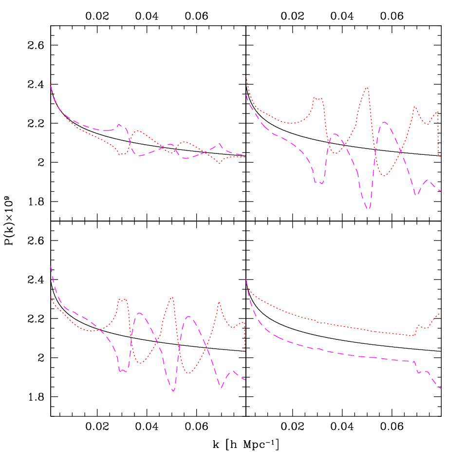
The cosmological parameters obtained from a traditional Markov Chain Monte Carlo search are used to give us our fiducial operator, . The parameters however have errors present upon them, which are not usually incorporated into errors on the final reconstructed . If inaccurate parameters have been used to calculate the fiducial operator very specific signatures would be expected to show up in the reconstructed from of . We show in Fig. 3 how these signatures appear in the reconstructed for anisotropies for four cosmological parameters, , , and . If any features with this form are observered one should attribute this to an incorrect estimation of the parameters and not some fundamental physics. A check for this would be if the corresponding features also show up in the reconstructed and spectra.
We have also tested the inversion on simulated CMB data with similar experimental properties as the recently launched Planck satelite mission [53]. We assume a total of 12 detectors with NETs of 64 observing 80% of the sky over 12 months with a resolution of 7 arcminutes FWHM. We calculate errors around our fiducial CMB best-fit models in both total intensity and polarisation spectra for this experimental setup and use these together with samples on the fiducial model to test the inversion method’s properties. We consider multipoles of for both total intensity spectra and polarisation. We have not taken into account any residual error from foreground subtraction in our forecasts. Thus our forecast are on the optimistic side of the accuracy achievable in the case of polarisation where foreground removal will certainly have a significant impact on errors at . In the case of total intensity spectra we are significantly underestimating the accuracy achievable by Planck as we expect to obtain well measured ’s well above of . We do not consider these modes as it significantly increases the time required to perform the SVD. Consideration of total-intensity modes past of will increase the accuracy obtainable for Planck on , it also allows one to probe past . It would be desirable to perform this process with a greater range when the Planck data becomes available.
To compare the accuracy obtainable with each of the anisotropy types we show the degree to which they each reconstruct a simple power law in Fig. 4. We use the same fiducial cosmological model as in Fig. 2 with a standard power law input equal to the spectra being reconstructed. All the were placed on the fiducial model. Over the whole range of total-intensity modes best constrain . But it is also true that there are regions in -space, for example between and , where considering only the measurements can give us a more accurate estimation of . measurements approach the accuracy of at a number of points, there are however regions where the errors become so large that any reconstructed is meaningless (these correspond to the troughs of the spectrum). The regions of -space corresponding to the most accurately measured regions are the peaks of the spectra. Both and spectra are not significantly affected by changes to at very low , so errors in this region are artificially small.
We also tested the combined and parameter estimation MCMC search as described in the previous section. The optimal binning method found bins for the Planck experiment, where our target signal-to-noise value in each bin is . We choose this value so as to have approximately the same number of bins across the range where WMAP best probes .
In Fig. 5 we show the results of a cosmological parameter estimation from this process for a simulated Planck experiment. We find that the input parameters were accurately recovered after this process. We show the final reconstructed in Fig. 6. The red line is the reconstructed at its best-fit point. The error bars we show are obtained from combining the error from the marginalised distributions with the reconstruction errors given the observed CMB data. The errors are centred around the mean of the marginalised distribution for each bin. It is important to note that the errors are highly correlated. This explains the reduced scatter in the mean values compared to the size of the plotted errors. As was seen in Fig. 3 changing a single parameter by a small amount (in the manner a MCMC search does) creates a very specific signature on for each parameter, where changing it slightly has a correlated effect upon the whole range of . This explains the very high correlations observed accross the whole range. It is at odds with the errors on associated with those of at any best-fit point which are not correlated across large ranges of .
IV Constraints from current CMB observations


We used two sets of currently available data to estimate the cosmological parameters in conjunction with a free unparameterised . The first is the WMAP 5-year data alone [54], in the second we combine this with that of SNIa, HST and BBN [55, 56, 57, 58, 59]. The second set combination chosen because the non-CMB sets do not depend upon the form of and can therefore give us independent and tighter constraints on most of the cosmological parameters. We run this data through the MCMC tool COSMOMC in the same manner as we did for the test Planck data.
In Fig. 7 we show the current constraints on , , and . The solid red vertical lines indicates the WMAP only best fit values when is parameterised in the usual fashion, the black solid curves represent the marginalised probability distribution of the WMAP only data. There is no disagreement between this and the WMAP bestfit model. The blue dotted line shows the marginalised probability distribution of WMAP including the other datasets. Here we observe some tension at around the level in . The inclusion of this data does not move the position of the likelihood peak significantly for each parameter.
The optimal binning method gave us 86 bins in our k range for WMAP. We used the minimum as described previously, this gave a target signal-to-noise ratio of . The binned reconstructed are shown in Figs. 8 and 9 for each of the two data sets. As in the Planck case, the results of the MCMC are highly correlated across the whole range, in contrast to a single reconstruction which is not. We have similarly added the errors from the MCMC to a single reconstruction in each bin in quadrature. The red lines are the reconstructed at their best-fit points. They error bars are centred around the best-fit marginalised value of each bin. For the WMAP only run we find that the limiting errors on in the range come from uncertainty in the cosmological parameters, whereas this limiting range is around when we include the other datasets. No significant deviation from the standard power-law case is observed in either run.
V Discussion
The SVD based reconstruction method we have outlined provides is fast enough to be incorporated into full MCMC parameter fitting runs. We have tested the method and shown that it recovers the overall features of input spectra. We have applied the method to forecasted Planck data and current WMAP 5-year results. These results have allowed us to consistently combine the reconstruction with a full exploration of the parameter likelihoods for the first time. We have seen that the limiting factor in constraining the primordial spectrum over a large range of wavenumbers comes from the uncertainty in cosmological parameters. Any claims of a detection of a feature in must necessarily confront the degeneracy with the cosmological parameter space . This effect will be less important when the Planck data is released, however it must still be considered as the unprecedented accuracy offered by future data may lead to premature claims of a detection of an interesting feature.
We observed some tension between the WMAP only best-fit model, when is parameterised with the normal amplitude and tilt, and our method in the marginalised probability distribution of . They disagree at around the level which is not overly significant, however it is an indication that there may be some departure from a standard power law in . Planck will certainly determine if this is the case.
There are other currently available CMB datasets, which could expand the range of probed. However expanding the method to include multiple data sets is a non-trivial task due to the binning of the data for sub-orbital experiments and the increased running time required for the expanded -range. We leave this analysis for future work.
In the future, as CMB polarisation data becomes increasingly accurate, it will be desirable to perform a joint inversion of total intensity data along with polarisation data. It is not clear how to extend the SVD based method to include all polarisation modes simultaneously since a HOSVD (Higher-Order SVD) step would probably be required. On the other hand this would give the best estimate of given any dataset and would help to reduce the correlations found in the reconstructed by increasing the degrees of freedom that can be effectively constrained.
Acknowledgements.
This work was supported by a STFC studentship. We acknowledge the use the Imperial College high performance computing service11 1 http://www.imperial.ac.uk/ict.References
- [1] A. A. Starobinsky, JETP Lett. 55, 489 (1992).
- [2] J. A. Adams, B. Cresswell, and R. Easther, Phys. Rev. D64, 123514 (2001), eprint astro-ph/0102236.
- [3] X. Wang, B. Feng, M. Li, X.-L. Chen, and X. Zhang, Int. J. Mod. Phys. D14, 1347 (2005), eprint astro-ph/0209242.
- [4] P. Hunt and S. Sarkar, Phys. Rev. D70, 103518 (2004), eprint astro-ph/0408138.
- [5] M. Joy, V. Sahni, and A. A. Starobinsky, Phys. Rev. D77, 023514 (2008a), eprint 0711.1585.
- [6] P. Hunt and S. Sarkar, Phys. Rev. D76, 123504 (2007), eprint 0706.2443.
- [7] C. Pahud, M. Kamionkowski, and A. R. Liddle (2008), eprint 0807.0322.
- [8] R. Lerner and J. McDonald, Phys. Rev. D79, 023511 (2009), eprint 0811.1933.
- [9] C. R. Contaldi, M. Peloso, L. Kofman, and A. Linde, JCAP 0307, 002 (2003), eprint astro-ph/0303636.
- [10] B. A. Powell and W. H. Kinney, Phys. Rev. D76, 063512 (2007), eprint astro-ph/0612006.
- [11] G. Nicholson and C. R. Contaldi, JCAP 0801, 002 (2008), eprint astro-ph/0701783.
- [12] J. Lesgourgues, Nucl. Phys. B582, 593 (2000), eprint hep-ph/9911447.
- [13] B. Feng and X. Zhang, Phys. Lett. B570, 145 (2003), eprint astro-ph/0305020.
- [14] G. J. Mathews, D. J. H. Chung, K. Ichiki, T. Kajino, and M. Orito, Phys. Rev. D70, 083505 (2004), eprint astro-ph/0406046.
- [15] R. K. Jain, P. Chingangbam, J.-O. Gong, L. Sriramkumar, and T. Souradeep, JCAP 0901, 009 (2009a), eprint 0809.3915.
- [16] A. E. Romano and M. Sasaki, Phys. Rev. D78, 103522 (2008), eprint 0809.5142.
- [17] R. K. Jain, P. Chingangbam, L. Sriramkumar, and T. Souradeep (2009b), eprint 0904.2518.
- [18] G. Nicholson and C. R. Contaldi (2009), eprint 0903.1106.
- [19] S. L. Bridle, A. M. Lewis, J. Weller, and G. Efstathiou, Mon. Not. Roy. Astron. Soc. 342, L72 (2003), eprint astro-ph/0302306.
- [20] D. Parkinson, S. Tsujikawa, B. A. Bassett, and L. Amendola, Phys. Rev. D71, 063524 (2005), eprint astro-ph/0409071.
- [21] R. Sinha and T. Souradeep, Phys. Rev. D74, 043518 (2006), eprint astro-ph/0511808.
- [22] C. Sealfon, L. Verde, and R. Jimenez, Phys. Rev. D72, 103520 (2005), eprint astro-ph/0506707.
- [23] P. Mukherjee and Y. Wang, JCAP 0512, 007 (2005), eprint astro-ph/0502136.
- [24] M. Bridges, A. N. Lasenby, and M. P. Hobson, Mon. Not. Roy. Astron. Soc. 369, 1123 (2006a), eprint astro-ph/0511573.
- [25] M. Bridges, A. N. Lasenby, and M. P. Hobson (2006b), eprint astro-ph/0607404.
- [26] L. Covi, J. Hamann, A. Melchiorri, A. Slosar, and I. Sorbera, Phys. Rev. D74, 083509 (2006), eprint astro-ph/0606452.
- [27] M. Joy, A. Shafieloo, V. Sahni, and A. A. Starobinsky (2008b), eprint 0807.3334.
- [28] L. Verde and H. V. Peiris, JCAP 0807, 009 (2008), eprint 0802.1219.
- [29] S. Hannestad, Phys. Rev. D63, 043009 (2001), eprint astro-ph/0009296.
- [30] Y. Wang and G. Mathews, Astrophys. J. 573, 1 (2002), eprint astro-ph/0011351.
- [31] M. Matsumiya, M. Sasaki, and J. Yokoyama, Phys. Rev. D65, 083007 (2002), eprint astro-ph/0111549.
- [32] A. Shafieloo and T. Souradeep, Phys. Rev. D70, 043523 (2004), eprint astro-ph/0312174.
- [33] N. Kogo, M. Matsumiya, M. Sasaki, and J. Yokoyama, Astrophys. J. 607, 32 (2004a), eprint astro-ph/0309662.
- [34] P. Mukherjee and Y. Wang, Astrophys. J. 593, 38 (2003a), eprint astro-ph/0301058.
- [35] P. Mukherjee and Y. Wang, Astrophys. J. 599, 1 (2003b), eprint astro-ph/0303211.
- [36] S. Hannestad, JCAP 0404, 002 (2004), eprint astro-ph/0311491.
- [37] N. Kogo, M. Sasaki, and J. Yokoyama, Phys. Rev. D70, 103001 (2004b), eprint astro-ph/0409052.
- [38] D. Tocchini-Valentini, M. Douspis, and J. Silk, Mon. Not. Roy. Astron. Soc. 359, 31 (2005), eprint astro-ph/0402583.
- [39] S. M. Leach, Mon. Not. Roy. Astron. Soc. 372, 646 (2006), eprint astro-ph/0506390.
- [40] A. Shafieloo, T. Souradeep, P. Manimaran, P. K. Panigrahi, and R. Rangarajan, Phys. Rev. D75, 123502 (2007), eprint astro-ph/0611352.
- [41] A. Shafieloo and T. Souradeep, Phys. Rev. D78, 023511 (2008), eprint 0709.1944.
- [42] R. Nagata and J. Yokoyama, Phys. Rev. D78, 123002 (2008), eprint 0809.4537.
- [43] R. Nagata and J. Yokoyama, Phys. Rev. D79, 043010 (2009), eprint 0812.4585.
- [44] W. Hu and T. Okamoto, Phys. Rev. D69, 043004 (2004), eprint astro-ph/0308049.
- [45] M. J. Mortonson, C. Dvorkin, H. V. Peiris, and W. Hu (2009), eprint 0903.4920.
- [46] U. Seljak and M. Zaldarriaga, Astrophys. J. 469, 437 (1996), eprint astro-ph/9603033.
- [47] A. Lewis, A. Challinor, and A. Lasenby, Astrophys. J. 538, 473 (2000), eprint astro-ph/9911177.
- [48] J. R. Bond, A. H. Jaffe, and L. E. Knox, Astrophys. J. 533, 19 (2000), eprint astro-ph/9808264.
- [49] P. Paykari and A. H. Jaffe (2009), eprint astro-ph/0902.4399.
- [50] A. Lewis and S. Bridle, Phys. Rev. D66, 103511 (2002), eprint astro-ph/0205436.
- [51] J. Martin and C. Ringeval, Phys. Rev. D69, 083515 (2004), eprint astro-ph/0310382.
- [52] J. Martin and C. Ringeval, JCAP 0501, 007 (2005), eprint hep-ph/0405249.
- [53] Planck: The scientific programme (2006), eprint astro-ph/0604069.
- [54] G. Hinshaw et al. (WMAP) (2008), eprint astro-ph/0803.0732.
- [55] S. Perlmutter et al. (Supernova Cosmology Project), Astrophys. J. 517, 565 (1999), eprint astro-ph/9812133.
- [56] A. G. Riess et al. (Supernova Search Team), Astrophys. J. 607, 665 (2004), eprint astro-ph/0402512.
- [57] P. Astier et al., Astron. Astrophys. 447, 31 (2006), eprint astro-ph/0510447.
- [58] M. Kowalski et al. (2008), eprint 0804.4142.
- [59] W. L. Freedman et al., Astrophys. J. 553, 47 (2001), eprint astro-ph/0012376.