Decays into Light Scalar Dark Matter
Abstract
We examine decays of a spin-1 bottomonium into a pair of light scalar Dark Matter (DM) particles, assuming that Dark Matter is produced due to exchange of heavy degrees of freedom. We perform a model-independent analysis and derive formulae for the branching ratios of these decays. We confront our calculation results with the experimental data. We show that the considered branching ratios are within the reach of the present BaBaR experimental sensitivity. Thus, Dark Matter production in decays leads to constraints on parameters of various models containing a light spin-0 DM particle. We illustrate this for the models with a ”WIMPless miracle”, in particular for a Gauge Mediated SUSY breaking scenario, with a spin-0 DM particle in the hidden sector. Another example considered is the type II 2HDM with a scalar DM particle.
1 Introduction
The origin, presence and nature of Dark Matter (DM) in our Universe remains one of the biggest mysteries of the particle physics and astrophysics [1]. Understanding the nature of Dark Matter, which accounts for majority of mass in the Universe, represents a crucial step in connecting astronomical observations with predictions of various elementary particle theories.
Many theories, the extensions of the Standard Model (SM), predict one or more stable, electrically-neutral particle(s) in their spectrum, which can be possible Dark Matter candidate(s). Different models provide different assignments for DM particles’ spin and various windows for their masses and couplings. To test this great variety of hypotheses, several techniques for DM direct or indirect search are currently developed.
Recent experimental measurements of Dark Matter relic abundance, by WMAP collaboration [2], can be used to place constraints on the masses and interaction strengths of DM particles. Indeed, the relation
| (1.1) |
with and being the mass and the interaction strength associated with DM annihilation, implies that, for a weakly-interacting particle, the mass scale should be set around the electroweak scale. This, coupled with an observation that very light DM particles might overclose the Universe (known as a Lee-Weinberg limit [3]) , seems to exclude the possibility of light weakly-interacting massive particle (WIMP) solution for DM, setting GeV.
A detailed look at this argument reveals that those constraints can be easily avoided in concrete models, so even MeV-scale particles can be good candidates for DM. For instance, low-energy resonances - such a light CP-odd Higgs in the MSSM extensions with a Higgs singlet, or a light extra gauge U-boson - could enhance the DM annihilation cross-section, without the need for a large coupling constant [4], [5], [6]-[9]. Even if no light resonances exist, the usual suppression of DM annihilation cross-section, , used in setting the Lee-Weinberg limit, does not hold, if Dark Matter is a non-fermionic (e.g. spin-0) state [6, 10, 11, 12, 13, 14, 15]. Furthermore, DM production could be non-thermal [16, 17], in which case the constraint provided by Eq. (.1) does not apply. Thus, models with light Dark Matter ( few GeV or less) still deserve a detailed and thorough study.
In this paper we consider the possibility of using of meson decays with missing energy, to test the models with a light spin-0 DM particle. Studies of heavy meson (and in particular meson) decays with missing energy may be especially valuable in light of the fact that DM direct search experiments, such as DAMA [18, 19, 20], CDMS [21] and XENON [22, 23], which rely on the measurement of kinematic recoil of nuclei in DM interactions, lose (for cold DM particles) sensitivity with decreasing mass of the WIMP, as the recoil energy becomes small. Of course, light Dark Matter may also be produced at high energy colliders, however the production rate is naturally going to be insensitive to precise value of the WIMP mass, if the one is much less than the beam center-of-mass energy [24]. Indirect experiments, such as HESS [25], are specifically tuned to see large energy secondaries, only possible for weak-scale WIMPs. The backgrounds for positron and antiproton searches by HEAT [26] and/or PAMELA [27, 28] experiments could be prohibitively large at small energies. Thus, (and/or other heavy meson) decays with missing energy may serve as alternative DM search channels, capable to provide us with an information on the WIMP mass range, hardly testable by the experiments discussed above.
So far, meson decays into Dark Matter have been considered within the models, where DM particles interaction with an ordinary matter is mediated by some light degree of freedom [4, 7, 29]. Apart from desire of having DM annihilation enhancement (due to a light intermediate resonance) and thus having no tension with the DM relic abundance condition, it is also known that meson SM decay is predominantly due to strong interactions. Thus, the WIMP production branching ratio, in general, is greatly suppressed compared to relevant weak B decays, and in particular to transition [11, 12]. In light of this, it might seem natural to concentrate only on the models within which Dark Matter production in decays is enhanced due to exchange of a light particle propagator.
Yet, the aim of the present paper is to study decay into a pair of spin-0 DM particles, , and decay into a pair of spin-0 DM particles and a photon, , within the models where light Dark Matter interaction with an ordinary matter is due to exchange of heavy particles (with masses exceeding the bottomonium mass). As it is mentioned above, these models may be free of tension related to satisfying the DM relic abundance constraint as well. Examples of such models will be discussed below. Also, new experimental data on decays into invisible states have been reported by the BaBaR collaboration [30, 31]. According to these data,
| (1.2) |
and
| (1.3) |
where the interval in the r.h.s. of Eq. (.3) is related to the choice of the final state missing mass. These bounds are significantly stronger than those on invisible decays (with or without a photon emission), reported previously by Belle and CLEO [32, 33] and quoted by Particle Data Group [34]. We show here that BaBaR experimental data on meson invisible decays (without or with a photon emission) may constrain the parameter space of light scalar Dark Matter models, even if there is no Dark Matter production enhancement due to light intermediate states.
We also illustrate (in Sections 5 and 6) that the study of Dark Matter production in decays allows us to test regions of parameter space of light spin-0 DM models that are inaccessible for B meson decays with missing energy. It is also worth mentioning that decays are sensitive to a wider range of WIMP mass than B decays. Thus, the study of WIMP production in decays is complementary to that for B meson decays.
Within the models where scalar DM consists of particles that are their own antiparticles, only transition is relevant. The transition rate of vanishes, if . Indeed, by angular momentum conservation, the produced DM particles pair in decay must be in a P-wave state, which is impossible because of the Bose-Einstein symmetry of identical spin-0 particles.
The scenarios with light complex scalar Dark Matter, albeit implying some continuous symmetry related to the internal charge of the complex (electrically) neutral scalar field, may be realized in many extensions of the Standard Model. Some of the models allow the scenarios both with a real and with a complex light scalar DM field [6, 13, 14, 15, 35]. Within these models, study of the decay represents an excellent opportunity to test the DM field nature either at present or in the future (if higher experimental resolution is needed).
As mentioned above, we restrict ourselves to the class of models where light spin-0 DM production is mediated by heavy degrees of freedom. At the energy scales, associated with decays, heavy intermediate degrees of freedom may be integrated out, thus leading to a low-energy effective theory of four-particle interactions. Our strategy would be deriving first model-independent formulae for the and branching ratios within the low-energy effective theory. Then, we confront our predictions with the experimental data, deriving model-independent bounds in terms of the Wilson operator expansion coefficients as the parameters that carry the information on an underlying New Physics (NP) model. Finally, within a given model, using the matching conditions for the Wilson coefficients, we translate these bounds into those on the relevant parameters of the considered model.
The paper is organized as follows. In Section 2 the general formalism is developed and model-independent formulae for the and branching ratios are derived. Both the case of complex and the case of self-conjugate DM field are considered. In Section 3 the neutrino background effect is discussed. We show that it has negligible impact on our analysis. In Section 4 we confront our calculation results with the experimental data and derive model-independent bounds on the Wilson coefficients. In the next sections we transform these bounds into constraints on the parameters of particular models. In Section 5 models with a complex spin-0 DM field are considered. We choose the class of mirror fermion models as an example. These models include, in particular, Gauge Mediated SUSY Breaking scenarios with the DM particle in the hidden sector and the mirror fermions being connectors between the hidden and the MSSM sectors [13, 14, 15]. An example of the self-conjugate DM scenario, two-Higgs doublet model with a scalar DM particle, is considered in Section 6. The concluding remarks are given in Section 7.
2 General Formalism: Model-Independent Formulae for the Decays Branching Ratios
We treat states - neglecting the sea quark and gluon distributions - as bound states of valence quark-antiquark pair that annihilates - with or without emission of a photon - into a pair of Dark Matter particles. To this approximation, the relevant low-energy effective Hamiltonian may be written as
| (2.1) |
where is the heavy mass and
| (2.2) |
with . It is worth noting that with the notations used in (.1) and (.2), all the operators , i=1,..4, are Hermitean, thus all the Wilson coefficients must be real. Another point to be made is that the are low-energy renormalization scale-independent. This stems from the renormalization scale invariance of the hadronic parts of operators , which - combined with the fact that DM particles do not interact strongly or electromagnetically - leads to low-energy scale invariance of and (from the scale invariance of the effective Hamiltonian) to that of . If DM consists of particles that are their own antiparticles, then only first two operators in Eq. (.2) would contribute.

To the considered approximation, the operator basis, given by Eq. (.2), is the most general one for the transition. With the use of the same basis, the other decay, , occurs by means of bi-local interactions depicted in Fig. 1 (a), (b). In principle, it is also possible - if the intermediate heavy states are (electrically) charged - that both the photon and the DM particles originate from the same effective vertex (Fig. 1 (c)). In order to take into account this diagram, higher dimension operators, involving electromagnetic field tensor, should also be included. However, such higher dimension operators would enter the expression for with higher powers of factor. Extra suppression of diagram in Fig. 1(c) in powers of the heavy mass inverse may be seen from the fact that one must introduce an extra heavy propagator or, equivalently, an extra power of or , as the photon is emitted by a heavy intermediate degree of freedom.
Thus, one may neglect contribution of the diagram in Fig. 1(c), as compared to that of the other two diagrams. This justifies the use of the operators basis, given by Eq. (.2), for decay as well.
In the rest frame of meson, matrix elements of the local hadronic currents may be parameterized at the origin, , as
| (2.3) |
where is the decay constant, is the mass, is the momentum and is the polarization vector of meson. Although the tensor current is not present in (.2), it inevitably appears in calculations of the amplitude. Thus, we need this current matrix element parametrization as well. Also, it is worth mentioning that due to the vector current conservation.
Non-local hadronic currents matrix elements may be expressed, to the leading order in expansion, in terms of those of the local currents in the following way:
| (2.4) |
where is a product of -matrices. This relationship is derived using the constituent quark approach, which assumes that within meson both and are static and have a mass each. Thus, one neglects difference between and as well as the quark-antiquark Fermi motion effects.
Let us proceed to the transition amplitudes and rates. As it is discussed above, to the leading order the decay occurs as a result of an effective local four-particle interaction. Thus, as it follows from (.1), (.2), (.3), only operator contributes to this decay. Furthermore, if is a real scalar (or pseudoscalar) state, it is easy to show that contribution of vanishes as well.
Calculation of branching ratio is straightforward: for being a complex scalar state one gets
| (2.5) |
where is the DM particle mass and [34] is the total width.
For being a self-conjugate spin-0 state, , one has
| (2.6) |
As it was mentioned above, this result is related to the fact that the final DM particle pair state must be a P-wave, which is impossible due to the Bose-Einstein symmetry of identical spin-0 particles. In what follows, must also vanish in higher orders in operator product expansion.
Thus, provided that DM pair production is the dominant invisible channel, the signal for decay would imply that the light spin-0 DM field has a complex nature. No evidence for the mode allows one to put some constraints on the parameters of the models with light complex scalar Dark Matter, as we illustrate in Sections 4 and 5.
Consider the other mode, . As it was mentioned above, this decay occurs as result of a bi-local interaction, and as direct calculations show the contribution of operator to the decay amplitude is vanishing, whereas the other operators have, in general, a non-zero contribution. In the case of being a complex scalar state, one gets
| (2.7) |
where
| (2.8) | |||
| (2.9) | |||
| (2.10) |
Here is the photon momentum, is the photon polarization vector, and are the momenta of the DM particle and antiparticle respectively (by momentum conservation, ).
Note that there is a difference in the phases of and . Thus, these parts of amplitude do not interfere. It is also easy to check, after doing some algebra, that there is no interference between and or as well. This is also easy to understand: contribution of the parity-conserving operator does not interfere with that of the parity violating operators and .
In what follows, the differential branching ratio for decay may be written in the following form:
| (2.11) |
where [34] is the total width and
| (2.12) | |||
| (2.13) |
Here is the electromagnetic coupling constant, and , where
is the missing mass squared. Note that the kinematically allowed range for the missing mass squared is . Subsequently, .
The partially integrated branching ratio for decay,
| (2.14) |
with or, equivalently, , is given by
| (2.15) |
where
| (2.16) | |||
| (2.17) |
We use the partially integrated branching ratio to confront the theoretical predictions with experimental data. The existing experimental bounds on mode are final state missing mass dependent [33, 31]. In particular, they may be very loose, or even there may be no bound, when the missing mass is close to its upper threshold, the mass. Thus, imposing a cutoff enables one to use existing experimental constraints on transition in the most efficient way. Also, this way one gets rid of the missing mass range, where the emitted photon energy is and non-perturbative QCD effects may be of importance. The price we pay is shrinking of the WIMP mass range, where our analysis is efficient.
Taking , one gets the total integrated branching ratio for decay:
| (2.18) |
where
| (2.19) | |||
| (2.20) |
The total integrated branching ratio may be used for theoretical studies, in particular to specify if a given model or class of models may be tested with the existing level of experimental accuracy.
In the case of being a real scalar (or pseudoscalar) state, contribution of vanishes and contributions of and to the branching ratio must be multiplied by factor two. In this case, one can rewrite formulae (.11) - (.20) in a more simple form:
| (2.21) |
| (2.22) |
and
| (2.23) |
As it was mentioned above, is the only mode that we use to test the models with self-conjugate spin-0 light Dark Matter.
3 Neutrino Background
In this section we consider neutrino-antineutrino pair production within and channels. We examine possible impact of the neutrino background on our analysis.
Neutrino background in and decays occurs due to and transitions. These transitions may occur both within the Standard Model and due to New Physics interactions. The NP contribution is model dependent and should be examined (upon necessity) in the framework of a particular model. Here we concentrate on the Standard Model contribution only. To the leading order within the SM, transition is mediated by virtual Z boson.
and transitions have been originally discussed in [36]. Later on has been studied in detail in [37], both within the Standard Model and within of some of its extensions. The SM result of ref. [37] may be rewritten in terms of branching ratio as
| (3.1) |
where is the Fermi coupling, is the weak mixing angle, and is the number of light non-sterile neutrinos. We use , , and [34]. The decay constant may be extracted from the experimental measurements of rate: one gets [38]. Using indicated values of the input parameters, one gets
| (3.2) |
Thus, decay branching ratio is about 30 times less than the BaBaR experimental bound on , given by Eq. (.2). In what follows, mode may be neglected in our analysis.
Calculation of branching ratio within the Standard Model is straightforward: it yields
| (3.3) |
and
| (3.4) |
where and [34], The decay constant may be found, using
| (3.5) |
where [34]. One gets and, subsequently,
| (3.6) |
Thus, branching ratio is about three orders of magnitude less than the BaBaR experimental limit on , given by Eq. (.3). In what follows, the effects related to decay may be neglected as well.
Thus, we may neglect the neutrino background effects when confronting theoretical predictions for decays into invisible states with the experimental data.
4 Model-Independent Bounds on the Wilson Coefficients
In this section we use our theoretical predictions and existing experimental data to derive model-independent constraints on the Wilson coefficients , i=1,2,3,4, as functions of DM particle mass, , and the heavy mass, .
We start with the bounds, coming from the study of decay. These bounds will be used in the next section, to constrain the models with light complex scalar Dark Matter. As follows from Eq. (.5), the decay branching ratio depends on the Wilson coefficient , the WIMP mass , the heavy mass , as well as on the mass, total width, and decay constant. The numerical values of , and have been specified in the previous section. Using these values, one gets
| (4.1) |
The uncertainty, about 4%, in the numerical factor in the r.h.s. of (.1) is due to that in the values of the input parameters. Such a small uncertainty may safely be neglected during the further analysis.
As it follows from Eqs. (.2) and (.1), branching ratio may be significantly greater than that of the transition. In what follows, decay into a pair of DM particles may be the dominant channel contributing to . Yet, in order to test this channel, the relevant experiments must be sensitive (at least) to . This sensitivity has been reached by the BaBaR experiment [30], as it follows from the bound on , given by Eq. (.2). Substituting (.2) into (.1), one derives the following constraint on as a function of and :
| (4.2) |


The behavior of the upper bound on with the DM particle mass is presented in Fig. 2(a). The bound on is almost insensitive to the WIMP mass for ; it grows rater slowly for ; however as , the bound starts increasing rapidly, due to the rapidly shrinking phase space. For and , the derived bound on may be translated into constraints on the relevant couplings of models with a light complex spin-0 DM field. For , the experimental sensitivity to transition must be improved to compensate the phase space suppression. Experimental sensitivity improvement is also necessary for higher values of the heavy mass : the upper bound on grows rapidly with the heavy mass, as it can be seen from Fig. 2(b) and as can be inferred from the quadratic dependence of this bound on .
Note that within specific models, the value of is somehow correlated to the values of the other Wilson coefficients, , and . In what follows, bound (.2) on may also lead to some constraints on , and , within particular models with a light complex spin-0 DM field. In terms of the branching ratios this means that experimental bound (.2) on (or on ) may lead to a phenomenological upper bound on , within particular models with a light complex spin-0 DM field.
At first glance, it may seem that a phenomenological upper bound on may have little practical use, in light of the existing BaBaR experimental constraint on , given by Eq. (.3). Yet, constraint (.3) is derived for the emitted photon having monochromatic energy: it has been assumed that transition is mediated by an intermediate resonant Higgs state [31]. Such a light Higgs state may exist e.g. within the extensions of the Minimal Supersymmetric Standard Model (MSSM) with an additional Higgs singlet [4, 5, 39]. Bounds of ref. [31] on have been plotted as a function of the mass of , or equivalently, of the final state fixed missing mass.

In the case of non-resonant DM production considered here, when the decay is mediated by heavy degrees of freedom, the final state missing mass (or the photon energy at rest frame) is not fixed. Instead, one has a broad missing mass distribution over the entire missing mass range, . For self-conjugate DM scenarios, the missing mass distribution shape is model-independent [as it is easy to see from Eq. (.21)] and is depicted in Fig. 3 for different choices of the WIMP mass. For complex scalar DM field scenarios, the missing mass distribution analysis depends on particular values of the Wilson coefficients [as one can see from Eqs. (.11)-(.13)] and hence on a particular model. It is however clear that apart from the endpoints, it is non-negligible for the entire missing mass range as well. In other words, the experimental analysis, performed in [31], should be extended to the cases, when the emitted photon energy is non-monochromatic and is in the range . To our knowledge, this work is in progress now11 1 The author is grateful to Yu. Kolomensky for this information..
Note that similar problems exist with the earlier bounds on , reported by CLEO [33]. Bound is derived assuming that is a single particle state. Thus, the emitted photon is monochromatic again. The only existing bound for the case of an invisible particle pair, , is too weak to produce any constraints within the models with non-resonant DM production. Due to the factor , is always below the quoted limit.
Of course, this all does not mean that the existing experimental constrains on are totally useless, if light spin-0 DM production is mediated by heavy non-resonant degrees of freedom. Note that BaBaR constraint (.3) on , except for being plotted as a function of the final state missing mass, may also be rewritten as a bound for a missing mass interval. One can see from versus plot of ref. [31] that
| (4.3) |
for or approximately , and provided that the emitted photon energy is monochromatic.
It has been discussed already that within the complex scalar DM field scenarios, one may derive a phenomenological upper bound on . Comparison of this bound with (.3) allows us to estimate if upcoming experimental constraints on , for the case of non-monochromatic photon emission, may further improve the existing constraints on the parameter space of a considered model. We will use this approach in the next section.
In this section, we concentrate hereafter on self-conjugate DM scenarios only. Recall that within these scenarios, transition rate vanishes, thus we are left with channel only. We perform the analysis of this decay channel, using the partially integrated branching ratio, for the missing mass interval, where bound (.3) is valid. We remind the reader that the insertion of a missing mass cut-off reduces significantly the WIMP mass range where an imposed experimental bound is efficient - we illustrate this in Fig. 4. Yet, as it has already been noted, all the existing bounds on have been derived for a restricted missing mass range or for a restricted invisible particle mass range (much below the kinematical threshold).

Using and [34] , , , one may rewrite formula (.22) for partially integrated branching ratio in the following form:
| (4.4) |
where
| (4.5) |
Note that , if , and if .
At first glance, it may seem from Eq. (.4) that branching ratio is far out of reach of the BaBaR experimental sensitivity, for a reasonable choice of and . Notice, however, that within certain models with light spin-0 Dark Matter, the Wilson coefficients and/or may be enormously large, as they contain some enhancement factors, such as the ratio - due to the mass term in the numerator of a heavy fermion propagator, or the Higgs vev’s ratio (with the latter being, say, ) - due to DM particle pair production via exchange of a heavy non-SM Higgs degree of freedom.
These enhancement factors can make and/or to be and hence to be , i.e. significantly exceeding bound (.3) on . Yet, bound (.3) assumes that the emitted photon energy is monochromatic: rigorously speaking, one should wait until the experimental limit on for the case of non-monochromatic photon emission comes out22 2 Also, the limit may be derived for state instead of - the author thanks Yu. Kolomensky for the discussion of this point. The reader, however, can easily check that making the replacements , and in formula (.22) modifies our predictions by about 25% only.. One may use (.3) only to derive a preliminary estimate of possible constraints on and hence on the relevant parameters of light spin-0 self-conjugate DM models.

This estimate may be presented as
| (4.6) |
It is also depicted in Fig. 5, as a function of , for . Based on the discussion above, this estimate implies rigorous constraints on the relevant parameters of the models with light spin-0 self-conjugate Dark Matter, for . We analyze these constraints within a particular model in Section 6.
5 Complex DM Field Scenarios: Mirror Fermion Models
As it was mentioned above, the distinct feature of the scenarios with a light complex spin-0 DM field is that decay rate is non-vanishing. One may use within these scenarios bound (.2) on , both to constrain the model parameter space, and - due to possible correlations in the values of the Wilson coefficients - to derive a phenomenological upper bound on the branching ratio.
Recall that bound (.2) on is strongest for and . Yet, even for these values of the heavy and WIMP masses, is still allowed to be of the order of unity. It seems to be very unlikely to saturate such a (rather weak) bound, if within a full electroweak theory, transition is loop-induced. We may therefore restrict ourselves by the models, where decay occurs at tree level.
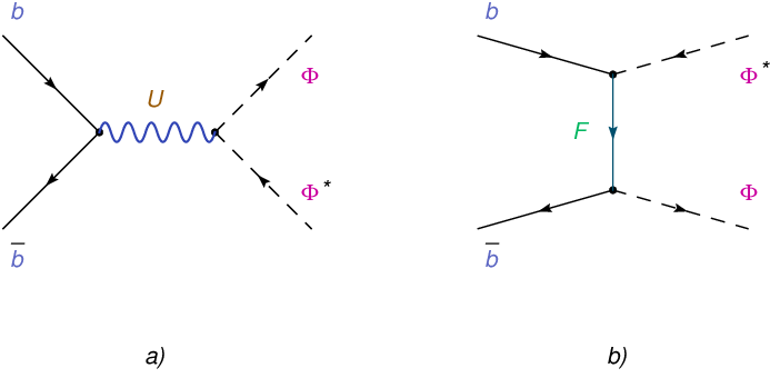
Possible tree level diagrams for transition within New Physics models are presented in Fig. 6. They involve exchange of either a neutral gauge boson or a charge -1/3 fermion. These type of diagrams may occur e.g. within U-boson models33 3 Scenarios with decaying into DM with a large rate through the SM Z boson may be excluded right away, as it would imply that Dark Matter contributes to the Z boson invisible width. or within mirror fermion models with light scalar Dark Matter [6, 7, 13, 14, 15].
Models with a new (beyond the SM) neutral gauge U-boson have been considered yet long ago, both within the supersymmetric theories and within the other SM extensions [40] - [44]. decays into invisible states (with or without a photon emission) have been studied in details in [29, 7, 45], within the scenarios with a light U-boson (with a mass less than a hundred MeV scale). In this paper only scenarios with a heavy U-boson are of interest. In that case, however, U-boson should be much heavier than the Z [6]. Both and branching ratios (inversely proportional to ) would be then suppressed too much to yield any constraints on the parameters of U-boson models.
Thus, we concentrate here only on the models with mirror fermions, where meson decays into Dark Matter by exchange of a heavy, charge -1/3 fermion, as shown in Fig. 6(b). Within these models, scalar Dark Matter couples to ordinary matter by means of Yukawa interactions, such as [6, 13]
| (5.1) |
where is a charge -1/3 colored mirror fermion. Unlike ordinary quarks, however, the right-handed component of transforms as a member of a weak isospin gauge doublet, while the left-handed component of transforms as a singlet. In other words, appears to be a mirror counterpart of b-quark. and other mirror fermions do not mix with ordinary quarks and leptons, as they - along with the DM particle - are odd under so-called M-parity [6], or mirror parity transformation, whereas ordinary matter is M-even. The scalar DM particle is the lightest M-odd particle of the theory.
Mirror fermion scenario may be realized [13, 14, 15] within the MSSM with gauge-mediated supersymmetry breaking and the DM particle in the hidden sector. It has been argued [13] that the thermal relic density constraint may be satisfied irrespectively of the DM particle mass and, in particular, within the light DM scenario (the ”WIMPless miracle”). As for the mirror fermions, they serve as connectors between the hidden and the MSSM sectors. For the sake of simplicity, it is assumed that each connector couples to one quark (or lepton), but other scenarios are in principle possible, where each mirror fermion has multiple couplings with the SM fermions, or each quark or lepton couples to multiple mirror fermions. The masses of mirror fermions are expected to be of the order of electroweak braking scale or heavier44 4 Unlike [13, 14, 46], we do not apply the bound on the fourth generation quark mass, [47]. In our opinion, this bound is irrelevant for the mirror fermion models. Indeed, constraints coming from the annihilation channel, , are invalid here: mirror fermions may annihilate to a DM particles pair (through interactions like that in (.1)) and hence escape detection. The other channel in use, , is also invalid, due to the mirror symmetry of the model., i.e. .
The tree level matching between the full and effective theories yields
| (5.2) |
where is the bottom mass evaluated at the matching scale. The natural choice of the matching scale is the heavy mass, , or, according (.2), . The bottom mass evolution with the scale is known up to four loops [48], yet to the leading-order approximation used here, it is given by
| (5.3) |
where [34].
Running of with the scale is the only QCD effect, relevant for our analysis. As it has been already mentioned above, the Wilson coefficients are low-energy renormalization scale-independent. That is to say, equations (.2) hold also at any scale , including the decay scale.
We begin with using (.2) to transform bound on , as a function of and , into that on the couplings and , as functions of and . This bound, in general, depends on possible correlations in the values of and . Here the following two scenarios are considered:
- •
the chiral scenario, when one of these coupling vanishes, e.g. ;
- •
non-chiral scenario, with .
Within the chiral scenario, the use of (.2) and (.2) yields
| (5.4) |
To the best of our knowledge, bound on the coupling (equivalently on , if we choose instead ) is derived for the first time. Dark Matter direct search experiments, based on DM scattering off nuclei, are sensitive to the light quark - mirror fermion interaction couplings only [13, 14]. So is the dominant contribution to DM annihilation processes. The decays or would inevitably depend both on and on , but not on alone. Other quarkonium, , invisible decay modes still need improvement of experimental sensitivity [46].
At first glance, bound (.4) on is weak. Furthermore, it is essential only for a restricted range of the mirror fermion mass: it becomes weaker than the perturbativity limit, , if . Nevertheless, the use of (.4) may lead to phenomenological upper bounds on some of bottomonium decay channels, and in particular, on .
Indeed, for the chiral scenario, matching conditions (.2) may be rewritten in the following form:
| (5.5) |
Thus, bound (.4) on may be transformed into the constraints on the Wilson coefficients and . Then, using formulae (.18) - (.20), for and the other parameters values specified in Sections 2 and 3, and applying the constraints on and , one derives an upper bound on (total) branching ratio, as a function of DM particle mass, .

We present this bound in Fig. 7. It may also be rewritten as , with the limit being saturated, as . Certainly, within the chiral scenario, is far away of the present experimental sensitivity. This result is not surprising: it has been anticipated in the previous section, for the models with no enhancement factors in the Wilson coefficients. The use of the derived constraint (.4) on enables one to formulate this quantitatively, by imposing a well defined limit on the branching ratio.

It is worth noting that a signal for the transition, above the quoted limit on , would rule out the mirror fermion models with light complex spin-0 Dark Matter and chiral mirror couplings. The following statement is also true: such a signal would imply that light spin-0 DM field is self-conjugate within the mirror fermion models with chiral mirror couplings. This result is not surprising as well: it has been noted previously that study of transition (combined with that of represents an opportunity to test, whether Dark Matter, if being light and a spin-0 state, is self-conjugate or complex.
Within the non-chiral scenario, , noting that , we may rewrite bound (.2) on in the following form:
| (5.6) |
We present this bound in Fig. 8, as a function of , for . The derived constraint on changes rather slowly with the WIMP mass, if . To simplify the analysis, one may use, within a crude approximation, for this range of the WIMP mass and . The behavior of bound (.6) with the mirror fermion mass is rather trivial ( grows linearly with ). We note here only that (.6) should be replaced by the perturbativity limit, , if .
Generally speaking, it is expected that ordinary-to-mirror fermion couplings be significantly less than one [6, 13]. If these couplings are of the same order for all three quark generations, one expects [6] from the DM relic abundance condition, . Otherwise, if a hierarchy in the couplings exists, one may argue that this expectation does not hold for : its value is not affected by the Dark Matter direct search designated experiments, nor does it have essential impact on DM annihilation and, hence, relic abundance. Furthermore, having a third generation Yukawa coupling to be of order unity is not unusual. However, bound (.6) on may be significantly improved due to possible constraints coming from the study of transition.
Indeed, within the non-chiral scenario, matching conditions (.2) may be rewritten for the Wilson coefficients , and as
| (5.7) |
Because of the enhancement factor , may be enormously large: as it has been discussed in Section 4, branching ratio is then within the reach of the present experimental sensitivity. Furthermore, due to this enhancement factor, roughly55 5 Slight deviation from this rule occurs due to running of the bottom mass with the heavy mass scale., unlike . Thus, within the non-chiral scenario, mode may be sensitive to a wider range of the mirror fermion mass than .
For the numerical analysis, we use . As it is mentioned above, this bound may be used in a crude approximation for and . In order to highlight the behavior of with the mirror fermion mass properly, we keep using for as well (even though the constraint on is significantly weaker then). This yields , and , for , and respectively, with the limits being saturated, as . We compare these limits to bound (.3) on . Recall that bound (.3) is derived for the emitted photon having monochromatic energy, thus it may be invalid for the scenarios where light DM is produced due to exchange of heavy non-resonant degrees of freedom. Yet, comparison of the above derived limits on to (.3) allows us to infer that upcoming BaBaR constraint on , for the case of non-monochromatic photon emission, may essentially improve the existing bound on .
If this constraint is of the same order as (.3), one would get , and , for sufficiently low WIMP mass and for , and respectively. The upcoming experimental data, however, may be not so optimistic, they may lead to a much weaker experimental limit than (.3). In either case, we want to emphasize again that we derive here preliminary estimates only of possible improvements of the existing bound on . More rigorously, regardless of any expectation, one must presently use the existing bound on , given by Eq. (.6).
To summarize our discussion of the mirror fermion models, we note that study of decay into a spin-0 DM particles pair, , leads - for the first time - to the bounds on the couplings of b-quark interaction with its mirror counterpart. Within the non-chiral scenario, these bounds may be somewhat improved by upcoming constraints on the mode for a non-monochromatic photon emission. Recall also that we assumed throughout this section that light spin-0 DM field has complex nature. Otherwise, within the self-conjugate DM scenario, no constraints on couplings, apart from preliminary estimates, may presently be derived.
6 Self-Conjugate DM Scenario: Dark Matter Model with two Higgs Doublets (2HDM)
In this section we will discuss the models, where interaction of (self-conjugate) spin-0 Dark Matter with the ordinary matter is mediated by heavy Higgs degrees of freedom. These models are known to be the most economical SM extensions, containing Dark Matter: they are created by extending (if necessary) the SM Higgs sector and embedding a scalar DM particle into theory, by adding a rather small number of unknown parameters.
The simplest model of this type is the Minimal Scalar Dark Matter Model [49, 50, 10]. It has the same particle content as the SM, plus a gauge singlet real scalar field , odd under discrete symmetry () and coupled to the SM particles through the exchange of Higgs boson. This model has been widely studied in the literature [10, 12, 11], [49]-[62]. Presently, the Minimal Scalar DM Model has a very restrained parameter space [10, 53, 12, 11], if the DM particle is chosen to have a GeV or smaller mass. Also, the decay channels considered here are not sensitive to the parameter space of this model. Indeed, as it has been shown in Section 4, for to be within the reach of the present experimental sensitivity, the Wilson coefficients and must contain some enhancement factors, such as heavy-to-light mass ratio or a large Higgs vev’s ratio. None of these enhancement factors may be generated in the Minimal Scalar Dark Matter Model, where DM particle production occurs solely via the SM Higgs boson exchange. Recall also that the other decay, , rate vanishes, when . Instead, the Minimal Scalar DM Model is well tested by mode, if assuming that DM particle has a GeV or smaller mass. Study of this mode leads to rigorous bounds on the model parameter space [11, 12].
In this section we consider the simplest extension of the Minimal Scalar DM Model, the two-Higgs doublet model (2HDM) with a gauge singlet real scalar DM particle. The DM interaction part of Lagrangian, relevant for our analysis, may be written as [11]
| (6.1) |
where is a odd real scalar DM field and
Following Refs. [11, 62], we consider type II version of 2HDM, where generates masses of down-type quarks and charged leptons, whereas generates masses of up-type quarks66 6 The used definition of and corresponds to the following notations for the Yukawa interactions: .. The Higgs vev’s, , , are constrained by the condition . The Higgs vev’s ratio, , is a free parameter of the theory. We assume here that . As discussed before, is then enhanced and may be within the reach of the BaBaR experimental sensitivity. Large scenarios are also known to be much less restrained than the Minimal Scalar DM Model. One may avoid tension with satisfying the DM relic density constraint. Another point worth mentioning is that the fine-tuning of parameters needed to generate a GeV or smaller DM mass is, in general, significantly weaker [11] than that within the Minimal Scalar DM Model.
After eliminating Goldstone modes, one may express and in terms of two CP-even, one CP-odd and two complex charged mass eigenstates - , , , respectively [63], [62]:
| (6.2) |
Here and are the lightest and heaviest CP-even states respectively, and is the CP-even mass-matrix diagonalization angle.
Using Eqs. (.2), one may rewrite (.1) in the following form:
| (6.3) |
where
| (6.4) |
is the DM particle mass,
| (6.5) | |||
| (6.6) |
and the ellipsis in (.3) stands for the dropped quartic interaction terms. To the leading order in the perturbation theory, transition occurs at tree level by exchange of a single Higgs boson. Thus, to the leading-order approximation, it is sufficient to consider only the cubic interaction terms in (.3). Then, as it follows from (.3), only the CP-even Higgs states are relevant for our analysis.
The b-quark Yukawa interaction terms may be written in the following form [63, 62, 34]:
| (6.7) |
where we write down explicitly only the b-quark interactions with the CP-even Higgs bosons.
Our strategy is the following now. We use (.3), (.5) - (.7), to derive the matching conditions for the Wilson coefficients and . Then, we transform bound (.6) on into that on the relevant couplings of the model, depending on the DM particle mass, Higgs mass and . We have to recall, however, that this bound may serve only as a preliminary estimate of possible constraints on the parameter space of the model.
In the limit of , the CP-even mixing angle has two possible solutions [63]:
- (a)
- (b)
In the former case (case a), the lightest CP-even Higgs boson, , is Standard Model-like: its phenomenology is similar to that of the SM Higgs boson and the experimental bound on its mass is close to the SM limit77 7 Also, if the SM Higgs decays predominantly invisibly, the SM lower experimental bound is distorted by a few GeV only [64, 65]. (see [34] and references therein).
In the latter case (case b), is ”New-Physics (NP) like”: its phenomenology differs drastically from that of the SM Higgs boson [63]. In particular, may be much below the Standard Model experimental limit: according the existing experimental data [66, 67], or in the general type II 2HDM.
As it was mentioned above, the light Higgs scenario is beyond the scope of the present paper, thus we assume here that . Notice, however, that this bound is derived, provided that no invisible Higgs decay mode exists. On the other hand, if the NP-like Higgs invisible decay mode is dominant, it may escape detection. No bound on , to our best knowledge, exists in that case.
Within the considered model with light scalar Dark Matter, analysis of the mode may restrict the scenarios with an invisibly decaying lightest Higgs boson by putting severe constraints on the interaction coupling, , given by Eq. (.5). If the lightest CP-even Higgs boson is NP-like (, case b), one may also rewrite (.5) as
| (6.8) |
The last term in the r.h.s. of (.8), although being suppressed by a factor of , must be retained because of possible hierarchy in the values of and or . Scenarios with such a hierarchy may be of importance, as is constrained to be , if mass approaches to its lower limit, .
Indeed, neglecting the heaviest SM-like CP-even Higgs exchange contribution, the matching conditions for the Wilson coefficients have the following form:
| (6.9) |
Thus, one may rewrite bound (.6) on as
| (6.10) |
where , , is given by Eq. (.5).

Formula (.10) implies a stringent upper bound on at the Higgs mass lower threshold, . Choosing e.g. , one has for the WIMP mass, , less than 2 GeV, as one can see from Fig. 9. For the other choice of the Higgs vev’s ratio, , the same constraint on is derived for , one also gets , as . For such small values of , it seems to be very unlikely that would escape detection and its mass be below 55 GeV. More rigorously, however, detailed reanalysis of the Higgs production and decay rates, including that of , should be performed (which is beyond the scope of the present paper).
Bound on may still be rigorous, if the mass is heavier than 55 GeV. For instance, choosing (in which case is still NP-like) and , one gets for , and for , . Yet, constraints become weaker with decreasing and increasing WIMP mass. It may be of order of the SM weak coupling, if and .
Thus, within the type II 2HDM with a light spin-0 Dark Matter, study of decay channel may lead to severe constraints on the lightest CP-even Higgs invisible decay coupling, if that Higgs is New-Physics like.
As it follows from Eq. (.8), bound (.10) on may also be transformed into that on the couplings , and . Constraints on and/or may also be derived from the study of transition [11]. Those, in general, are strong enough: in particular, values of and for are ruled out, if . In that case, suppressed terms in Eq. (.8) may safely be neglected, so that . In other words, bound (.10) on is also that on , if .
Note that due to cancellation effects in the relevant diagrams, WIMP pair production rate in B meson decays is insensitive to the value of [11], and hence, in general, to the value of . The scenarios with dominant, or at least non-negligible, have been thus far unconstrained. To our best knowledge, bound on the interaction coupling, , is derived for the first time. Thus, study of DM production in decays enables one to test the regions of the parameter space of 2HDM with scalar Dark Matter, which are inaccessible by B meson decays with missing energy.
It may seem naively that the rigorous constraint on the interaction coupling, , results also to suppress the DM annihilation rate, which in its turn may lead to scenarios with overabundant Dark Matter. Yet, the DM annihilation rate to down-type quarks and charged leptons is enhanced by a factor of (due to enhancement of these fermions Yukawa interaction with the CP-even Higgs, if the one is NP-like). Or, equivalently, using the notations of ref. [11], the effective coupling for these annihilation processes is
In terms of the coupling , bound (.10) may be rewritten as
| (6.11) |
Keeping in mind that or, equivalently, , bound (.11) on yields no essential constraints on DM annihilation and, hence, no tension with satisfying DM relic abundance constraint above the Lee-Weinberg limit of the model, [11]. Thus, the 2HDM scenario with dominant, or at least non-negligible, is much less restrained, than those with or dominant or than Minimal Scalar DM Model [11, 12].
So far it has been assumed that the lightest CP-even Higgs boson is NP-like. In the opposite case, when is the SM-like (case a), the matching between the full and effective theories yields
| (6.12) |
In deriving (.12), we used, for and ,
| (6.13) |
It is not hard to see from our further analysis that omitted terms in Eqs. (.13) are not essential in this case.
The first term in the expression for is due to the SM-like Higgs exchange. As expected, it has no enhancement factor - thus, as it was discussed in Section 4, contribution of this term to the rate is by (at least) an order of magnitude lower than the present experimental sensitivity. We may further disregard the Dark Matter interaction with the lightest CP-even Higgs . Then, we may rewrite matching conditions (.12) in a more transparent form:
| (6.14) |
In other words, we restrict ourselves by considering the contribution to amplitude due to exchange of the heaviest (NP-like) Higgs boson only. This contribution is enhanced by factor, coming from Yukawa interaction coupling in (.7) (if ). The remarkable feature of the considered scenario is that even though transition is generated by exchange of the heaviest CP-even Higgs boson, the decay branching ratio for a certain range of mass is well within the reach of the present experimental sensitivity, due to enhancement. As a consequence, one may derive constraints on the coupling , as a function of , and .
Indeed, using Eqs. (.14), one may rewrite bound (.6) on as
| (6.15) |
Choosing as a reference value is not accidental. Within the general type II 2HDM, theoretical upper bound restricts the SM-like Higgs to be less than 180 GeV [68]. Also, the SM Higgs mass interval has been recently excluded with 95% C. L. by the CDF and D0 data [69]. Thus, within type II 2HDM, above 160 GeV, the CP-even Higgs boson is presumably the heaviest one and NP-like.


As one can see from Eq. (.15) and Fig. 10(a), for and , is constrained to be of order of the SM weak coupling or smaller (), if . Also, for the same choice of the Higgs mass and , is to be less than one, if the WIMP mass is less than 2 GeV. Bound on is significantly more rigorous for higher values of . For instance, if choosing , one gets and for and respectively.
The restrictions on are essential also for higher values of the heaviest CP-even Higgs mass: for , they are still of interest up to , as one can see from Fig. 10(b). Our analysis may be spread for the range as well, leading to more rigorous constraints than those in Fig. 10.
Recall that bound on is derived for the first time. It is also worth noting that constraints on imply also those on the heaviest CP-even Higgs invisible decay rate, if that Higgs is NP-like. As it follows from Eq. (.13), is the interaction coupling in this case. Yet, as in the case (b), bound (.15) does not seem to have an impact on the DM annihilation rate (which is enhanced). Vice versa, DM annihilation processes (and possibly scattering off nucleons) may lead to additional constraints on . Study of these processes, however, goes beyond the scope of the present paper.
Thus, within type II 2HDM with a scalar Dark Matter, for large scenario, meson decay into a Dark Matter particles pair and a photon, , may be used to derive essential constraints on the parameters of the model, which otherwise cannot be tested by B meson decays with invisible outcoming particles.
7 Conclusions and Summary
Thus, spin-0 Dark Matter production in meson decays has been investigated. We restricted ourselves by consideration of the models where the decays occur due to exchange of heavy non-resonant degrees of freedom. Both the scenarios with a complex scalar DM field and those with DM particle being its own antiparticle have been analyzed.
We performed our calculations within low-energy effective theory, integrating out heavy degrees of freedom. This way we derived model-independent formulae for the considered branching ratios. We used these formulae to confront our theoretical predictions with existing experimental data on invisible decays, both in a model-independent way and within particular models. It has been shown that within the considered class of models, DM production rate in decays is within the reach of the present experimental sensitivity. Thus, meson decays into Dark Matter, with or without a photon emission, may be used to constrain the models with a GeV or lighter spin-0 DM. In particular, within the mirror fermion models, using the existing BaBaR constraint on the mode, we derived for the first time bounds on the parameters of the model that otherwise could not be tested by other DM search processes.
Experimental constraints on the other mode, , are derived assuming that Dark Matter is produced by exchange of a light resonant scalar state. Within the scenarios with non-resonant DM production, these constraints may be used only to make preliminary estimates of possible bounds on the parameters of the models. Yet, those estimates show that these bounds may be rigorous enough; besides, they are derived within the least restrained presently light scalar DM scenarios. Our goal is thus to encourage the experimental groups to analyze the experimental data on also for the case of non-monochromatic photon emission and spin-0 invisible states.
So, from our analysis one may conclude that Dark Matter production in meson decays may serve as an interesting alternative to commonly used DM search methods, capable of providing a valuable information on DM particles, if those turn to have a mass of the order of a few GeV or smaller.
Acknowledgements.
The author is grateful to Yu. Kolomensky, A. Blechman, A. A. Petrov, B. McElrath and J. Cao for valuable comments and stimulating discussions. The author thanks A. Badin for verifying some of derivations.This work has been supported by NSF Grant No. PHY-0547794 and DOE Grant No. DE-FGO2-96ER41005.
References
- [1] G. Bertone, D. Hooper, J. Silk, Phys. Rep. 405, 279 (2005).
- [2] J. Dunkley et al., (WMAP Collaboration), Astrophys. J. Suppl. 180, 306 (2009).
- [3] B. W. Lee and S. Weinberg, Phys. Rev. Lett. 39, 165 (1977); M. I. Vysotsky, A. D. Dolgov and Y. B. Zeldovich, JETP Lett. 26, 188 (1977) [Pisma Zh. Eksp. Teor. Fiz. 26, 200 (1977)].
- [4] J. F. Gunion, D. Hooper, B. McElrath, Phys. Rev. D73, 015011 (2006).
- [5] J. Cao, H. E. Logan, J. M. Yang, Phys. Rev. D 79, 091701 (2009).
- [6] C. Boehm, P. Fayet, Nucl. Phys. B 683, 219 (2004).
- [7] P. Fayet, Phys. Rev. D 75, 115017 (2007).
- [8] Y. Kahn, M. Schmitt, T. M. P. Tait, Phys. Rev. D 78, 115002 (2008).
- [9] D. Hooper, K. M. Zurek, Phys. Rev. D 77, 087302 (2008).
- [10] C. P. Burgess, M. Pospelov, T. ter Veldhuis, Nucl. Phys. B 619, 709 (2001).
- [11] C. Bird, R. Kowalewski, M. Pospelov, Mod. Phys. Lett. A 21, 457 (2006).
- [12] C. Bird, P. Jackson, R. Kowalewski, M. Pospelov, Phys. Rev. Lett. 93, 201803 (2004).
- [13] J. L. Feng, J. Kumar, Phys. Rev. Lett. 101, 231301 (2008).
- [14] J. L. Feng, J. Kumar, L. E. Strigari, Phys. Lett. B 670, 37 (2008).
- [15] J. L. Feng, J. Kumar, I. Learned, L. E. Strigari, JCAP 0901, 032 (2009), arXiv:0808.4151[hep-ph].
- [16] G. Kane and S. Watson, Mod. Phys. Lett. A 23, 2103 (2008).
- [17] B. S. Acharya, P. Kumar, G. Kane, S. Watson, arXiv:0908.2430 [astro-ph.CO].
- [18] R. Bernabei et al., (DAMA Collaboration) Eur. Phys. J. C 56, 333 (2008).
- [19] R. Bernabei et al., (DAMA Collaboration) Int. J. Mod. Phys. D 13, 2127 (2004).
- [20] R. Bernabei et al., (DAMA Collaboration) Riv. Nuovo Cimento, 26 N1, 1 (2003), arXiv:astro-ph/0307403.
- [21] Z. Ahmed et al., CDMS Collaboration, Phys. Rev. Lett. 102, 011301, (2009).
- [22] J. Angle et al. (XENON Collaboration) Phys. Rev. Lett. 101, 091301 (2008).
- [23] J. Angle et al. (XENON Collaboration) Phys. Rev. Lett. 100, 021303 (2008).
- [24] B. McElrath, ECONF-C070805, arXiv:0712.0016 [hep-ph].
- [25] F. Aharonian et al., HESS Collaboration, Astrophys. J. 691, 175 (2009), arXiv:0809.3894 [astro-ph].
- [26] S. W. Barwick, HEAT Collaboration, Astrophys. J. 482, L191 (1997).
- [27] O. Adriani, et al., (PAMELA Collaboration) Nature 458, 607 (2009).
- [28] O. Adriani, et al., (PAMELA Collaboration) Phys. Rev. Lett. 102, 051101 (2009).
- [29] P. Fayet, Phys. Rev. D 74, 054034 (2006).
- [30] The BaBaR Collaboration, B. Aubert et al., arXiv: 0908.2840 [hep-ex].
- [31]
The BaBaR Collaboration, B. Aubert et al., arXiv: 0808.0017 [hep-ex];
S. J. Sekula, for the BaBaR Collaboration, arXiv: 0810.0315 [hep-ex]. - [32] O. Tajima et al., The Belle Collaboration, Phys. Rev. Lett. 98, 132001 (2007).
- [33] R. Balest et al., CLEO Collaboration, Phys. Rev. D 51, 2053 (1995).
- [34] C. Amsler et al. (Particle Data Group), Phys. Lett. B 667, 1 (2008).
- [35] V. Barger et al. Phys. Rev. D 79, 015018 (2009).
- [36] L. Bergstrm, H. Rubinstein, Phys. Lett. B 201, 283 (1988).
- [37] L. N. Chang, O. Lebedev, J. N. Ng, Phys. Lett. B 441, 419 (1998).
- [38] H. M. Choi, Phys. Rev. D 75, 073016, (2007).
- [39] R. Dermisek, J. F. Gunion, B. McElrath, Phys. Rev. D 76, 051105 (2007); R. Dermisek, J. F. Gunion, Phys. Rev. D 75, 075019 (2007); R. Dermisek, J. F. Gunion, Phys. Rev. D73, 111701 (2006).
- [40] P. Fayet, Phys. Lett. B 95, 285 (1980).
- [41] P. Fayet, Nucl. Phys. B 187, 184 (1981).
- [42] P. Fayet, Phys. Lett. B 227, 127 (1989).
- [43] P. Fayet, Nucl. Phys. B 347, 743 (1990).
- [44] P. Fayet, Class. Quant. Grav. 13, A19 (1996).
- [45] P. Fayet, arXiv:0812.3980 [hep-ph].
- [46] D. McKeen Phys. Rev. D 79, 114001 (2009), arXiv:0903.4982 [hep-ph].
- [47] G. D. Kribs, T. Plehn, M. Spannowsky, T. M. P. Tait, Phys. Rev. D 76, 075016 (2007).
- [48]
K. G. Chetyrkin, Phys. Lett. B 404, 161 (1997);
J. A. M. Vermaseren, S. A. Larin, T. van Ritbergen, Phys. Lett. B 405, 327 (1997). - [49] V. Silveira, A. Zee, Phys. Lett. B 161, 136 (1985).
- [50]
J. McDonald, Phys. Rev. D 50, 3637 (1994);
J. McDonald, Phys. Rev. Lett. 88, 091304 (2002). - [51] M. C. Bento, O. Bertolami, R. Rosenfeld, L. Teodoro, Phys. Rev. D 62, 041302 (2000).
- [52] D. E. Holz, A. Zee, Phys. Lett. B 517, 239 (2001).
- [53] M. C. Bento, O. Bertolami, R. Rosenfeld, Phys. Lett. B 518, 276 (2001).
- [54] H. Davoudiasl, R. Kitano, T. Li, H. Murayama, Phys. Lett. B 609, 117 (2005).
- [55] G. Cynolter, E. Lendvai, G. Pocsik, Acta Phys. Polon. B 36, 827 (2005), arXiv:hep-ph/0410102.
- [56] Shou-Hua Zhu, Chin. Phys. Lett. 24, 381 (2007), arXiv:hep-ph/0601224.
- [57] V. Barger et al., Phys. Rev. D 77, 035005 (2008).
- [58] S. Andreas, T. Hambye, M. H. G. Tytgat, JCAP 0810:034 (2008), arXiv:0808.0255 [hep-ph].
- [59] C. E. Yaguna, JCAP 0903:003 (2009), arXiv:0810.4267 [hep-ph].
- [60] A. Goudelis, Y. Mambrini, C. Yaguna, arXiv:0909.2799 [hep-ph].
- [61] X. G. He, T. Li, X. Q. Li, H. C. Tsai, Mod. Phys. Lett. A 22, 2121 (2007).
- [62] X. G. He et al., Phys. Rev. D 79, 023521 (2009) .
- [63] J. F. Gunion, H. E. Haber, G. Kane, S. Dawson, The Higgs Hunter’s Guide, Addison-Wesley Publishing Company, 1990.
- [64] J. Abdallah, et al., DELPHI Collaboration, Eur. Phys. Journal C32, 475, (2004).
- [65] P. Achard et al., L3 Collaboration, Phys. Lett. B 609, 35 (2005).
- [66] G. Abbiendi et al., The OPAL Collaboration, Eur. Phys. Journal C 40, 317 (2005).
- [67] G. Abbiendi et al., The OPAL Collaboration, Eur. Phys. Journal C 18, 425 (2001).
- [68] G. M. Asatrian, A. N. Ioannisian, S. G. Matinyan, Sov. J. Nucl. Phys. 53, 371, (1991), Yad. Fiz. 53, 592, (1991).
- [69] D. Benjamin, for the CDF, D0 Collaborations, arXiv: 0906.1403 [hep-ex].