Simulations of Doppler Effects in Nuclear Reactions for AGATA Commissioning Experiments

According to the Pauli principle the fermions cannot occupy the same quantum state. Therefore nucleons can orbit almost freely inside the nucleus, similarly to the electrons in the atom. In the atom, electrons are moving in a central potential caused by the positively charged nucleus. In the nucleus, the potential is created by the nucleons themselves through the nucleon-nucleon interaction. In the shell model, the nucleons move in a central potential usually parametrized as

The first term in equation 2.1 is the Woods Saxon potential with the parameters: potential depth $V_{0}$, diffuseness parameter $a$, nuclear radius $R=r_{0}A^{2/3}$ ($A$ is the nucleon number and $r_{0}$ is the radius parameter). The second term is the spin-orbit interaction, where the spin ($\overrightarrow{s}$) and angular momentum ($\overrightarrow{\ell}$) vectors can be oriented either parallel or anti-parallel in the total nucleon spin quantum number $\overrightarrow{j}=\overrightarrow{\ell}\pm\frac{1}{2}$.

The single-particle model is an extreme shell model form where the nucleons move freely in a central potential without interacting with each other. An odd-$A$ nucleus in this model is composed of an inert even-even core, plus an unpaired nucleon. The last unpaired nucleon determines the nuclear properties, such as spin and parity. All known even-even nuclei have spin and parity $J^{\pi}=0^{+}$ in the ground state. By introducing a residual force in the shell model, called pairing, one can explain the ground state spin and parity of even-even nuclei. The pairing interaction implies an attractive force between pairs of nucleons with opposite orbital angular momenta in identical orbits. The strongest attractive interaction occurs for nucleon pairs with largest possible quantum numbers $m_{j}$ of opposite sign, i.e. $m_{j}=+j$ and $m_{j}=-j$. The quantum number $m_{j}$ is the projection of $j$ on a quantization axis and can have values from $-j$ to $j$. The spin and parity of each pair of nucleons in identical orbits with $\pm m_{j}$ is $0^{+}$. The attractive pairing interaction leads to an increase of the binding energy for a completely paired nucleus with total spin and parity $0^{+}$, compared with one with any number of non-paired nucleons.

The shell model can explain the presence of magic proton ($Z$) and neutron ($N$) numbers in the nuclei. By including the spin-orbit term in the potential, the shell model gives the magic numbers $Z,\>N=$ 2, 8, 20, 28, 50, 82, 126, which corresponds to strongly bound nuclei at filled shells. Experimental results verify these theoretical shell model predictions. Doubly magic nuclei have magic proton and neutron numbers. The few nuclei which are doubly magic are strongly bound, like e.g. ${}^{4}\mathrm{He}$.

Two major modes of collective excitations are described within this model, namely vibrational and rotational excitations [3].

In a direct reaction the projectile can undergo stripping in which case some of the nucleons are transferred from the projectile to the target. An example of a stripping reaction is (d,p). A knockout reaction can also occur, in which the incident nucleus knocks out nucleons from the target nucleus, as in a (p,np) reaction. Direct reactions occur on a very short time scale, $10^{-22}$ to $10^{-23}$s [3], and do not change the structure of the projectile and the target dramatically.

According to [5], compound nucleus reactions occur when two nuclei form an intermediate state. The compound nucleus formation between nuclei a and A is depicted as

where $X^{*}$ is the excited compound nucleus and R is the excited residual nucleus. The timescales of these reactions are relatively long, roughly $10^{-16}$ to $10^{-18}$s. The information about the constituents before the collision is permanently destroyed, hence the output decay channels is independent of the compound nucleus formation. If the same compound nucleus is reached through another reaction, say $c+C\rightarrow X^{*}$with different colliding nuclei, the probability of the decay channel $X^{*}\rightarrow R^{*}+\sum\mathrm{particles}$ remains the same. This hypothesis is called the independence hypothesis and it implies that it is possible to separate the cross section $\sigma$, into the formation cross section $\sigma_{\mathrm{aA}}^{\mathrm{CN}}$ for projectile a and target A, and the branching ratio $G_{\mathrm{Bb}}^{\mathrm{CN}}$ (CN=compound nucleus) for the decay to particle b and nucleus B:

The cross section term $\sigma_{\mathrm{Aa}}^{\mathrm{CN}}(E)$ is the probability of the compound nucleus formation at the center of mass energy $E$. As the compound nucleus must decay, the sum of all the partial decays is $\underset{i}{\sum}G_{i}^{\mathrm{CN}}(E)=1$. The excitation energy $E_{\mathrm{CN}}^{*}$ of the compound nucleus can be expressed as

where $E_{\mathrm{lab}}$ is the kinetic energy of the projectile in the laboratory frame and the masses $m_{a}$, $m_{A}$ and $m_{CN}$ are the atomic masses of the projectile, target, and compound nucleus, respectively. The compound nucleus de-excites through particle evaporation.

When irradiating a metal surface with light above a certain frequency, an electric current will flow. Einstein found that electrons are removed from the metal and that the photon is absorbed by the atom [10]. The photo-electron can only be ejected when the photon energy is higher than the binding energy of the electron. The kinetic energy for the photoelectron is given by

where $E_{\gamma}$ is the photon energy and $B_{e}$ is the electronic binding energy. The photoelectric effect dominates at low $E_{\gamma}$ (see figure 3.1).

When the photon energy increases, the probability of photon scattering with electrons increases (see figure 3.1). According to Compton in his article from 1923 [11], the observed photon wavelength $\lambda$ increases after the interaction, leading to a decreasing energy, since $E=hc/\lambda$. Recoil energy is transferred from the photon to the electron. Due to energy and momentum conservation, one arrives at the Compton scattering formula which gives the energy of the scattered $\gamma$ ray

Here $E_{\gamma}$ is the initial energy of the $\gamma$ ray, and $m$ is the mass of the electron. the scattering angle of the photon is $\theta_{\mathrm{C}}$.

If the photon energy is large enough, pair production may occur, i.e. creation of an electron-positron pair, as $\gamma\rightarrow\mathrm{e}^{+}+\mathrm{e}^{-}$. The minimum energy required is 1.022 MeV. Due to momentum and energy conservation this process is only possible if it occurs nearby a particle with non-zero rest mass, e.g. a nucleus [12].

The intensity of a beam passing through matter, decreases exponentially

where $I_{0}$ is the incident beam intensity, $\mu$ is the total attenuation coefficient and $\delta$ is the material thickness. The probability for a photon removal per unit length is given by $\mu$. The total attenuation coefficient is the sum of the attenuation coefficients for the photoelectric effect $\left(\tau\right),$ Compton scattering $\left(c\right)$ and pair production $\left(\kappa\right)$

The inverse of the attenuation coefficient is equal to the mean free path of the $\gamma$ rays

The high-purity germanium (HPGe) detector is undoubtedly the most successful instrument for spectroscopic studies of the nuclear structure. The superior performance of the HPGe detector is mainly due to its excellent energy resolution, which allows the distinction of $\gamma$ rays with close lying energies. The energy resolution is characterized by the full width at half maximum (FWHM) of the $\gamma$-ray peaks. Two factors contribute to the FWHM, here labeled $W$ [15]:

The intrinsic width $W_{\mathrm{i}}$ is caused by the properties of the detector itself and consists of three terms: the electronic noise $W_{\mathrm{en}}$, which is independent of the measured $\gamma$-ray energy, the statistical factor $W_{\mathrm{sf}}$, which depends on the square root of the energy, and the incomplete charge collection $W_{\mathrm{cc}}$, which is proportional to the energy,

The second factor $W_{D}$ is due to the Doppler effects and it is non-zero only if the $\gamma$ ray is emitted by a moving source. The Doppler factor consists of three terms:

$W{}_{\theta_{\gamma}}$ is due to the broadening caused by the uncertainty in the determination of the emission angle of the $\gamma$ ray, $\theta_{\gamma}$. This term depends on the position resolution of the first interaction point in the detector. The terms $W{}_{\mathrm{\theta_{r}}}$ and $W{}_{v_{\mathrm{r}}}$ are due to the uncertainty in the determination of the angle and velocity, respectively, of the residual nucleus.

When the ions enter the target material they are deflected due to the electromagnetic interaction primarily with the electrons. Thus, the ions will loose energy and deviate from the beam direction, which leads to so called energy and angular straggling of the ions. There are two main aspects of the target effects in the simulations.

1. 1.

   Position of the reaction in the target. If the reaction occurs in the beginning of the target, the residual nucleus will experience energy and angular straggling, whereas if the reaction occurs at the end, the incident ion instead of the residual nucleus will lose kinetic energy. The difference both in kinetic energy and atomic number of the incident ion and residual nucleus leads to the difference in straggling.

2. 2.

   Neutron energy and angular distribution. After the reaction the excited compound nucleus is formed, and particles are emitted. Depending on the energy and angular distribution of the particles, the residual nucleus will obtain different kinetic energies. The recoil due to the neutron evaporation will either boost the nucleus or slow it down. Since this happens inside the target material the energy and angular straggling will change after the reaction. Two extreme cases were investigated, one where the neutron is emitted at about $0^{\mathrm{o}}$ relative to the ion beam, and the other where it is emitted in at about $180^{\mathrm{o}}$.

In table 6.1 two reactions were shown with a dominating neutron emission channel. These are the reactions that were further studied. Both reactions leads to an even-even residual nucleus, and they have appropriate life times. The first reaction, $\mathrm{{}^{37}Cl\left(d,n\right){}^{38}Ar}$, leads to ${}^{38}\mathrm{Ar}$ which has a first excited state $2^{+}$ at 2168 keV. The high $\gamma$-ray energy which decays to the $0^{+}$ ground state is very good for the Doppler-effect measurements. The cross-section calculation from TALYS is shown in the upper plot of figure 6.5. The reaction $\mathrm{{}^{37}Cl(d,n)^{38}Ar}$ is clearly dominating.

The second reaction, $\mathrm{{}^{51}V\left(d,n\right){}^{52}Cr},$ is for the same reason a suitable reaction. The first excited state has an excitation energy of 1434 keV. The calculated cross section for this reaction is shown in the lower plot of figure 6.5.

The cross section of the reaction ${}^{37}\mathrm{\mathrm{Cl}\left(d,n\right)}\mathrm{{}^{38}Ar}$ reaches a maximum of about 350 mb at a deuteron energy of about 4 MeV. The cross section of the $\mathrm{{}^{51}V\left(d,n\right){}^{52}Cr}$ reaction has a local maximum at about $\mathrm{E_{d,LAB}=3}.4$ MeV and it increases at higher energies without competition with other channels. Based on the TALYS results, both reactions, $\mathrm{d+^{37}Cl}$ and $\mathrm{d+^{51}V}$, are suitable for further studies. The energies chosen are $E_{d}=3.8$MeV and $E_{d}=3.2$MeV for the $\mathrm{d+^{37}}\mathrm{Cl}$ and $\mathrm{d}+^{51}\mathrm{V}$ reactions respectively. In inverse kinematics reactions thus correspond to $E_{37_{\mathrm{Cl}}}=70.0$ MeV and $E_{51_{\mathrm{V}}}=81.6$ MeV, respectively.

To verify the calculations, a comparison between TALYS and evapOR was made. The results for the $\mathrm{d+^{51}V}$ reaction are presented in figure 6.6.

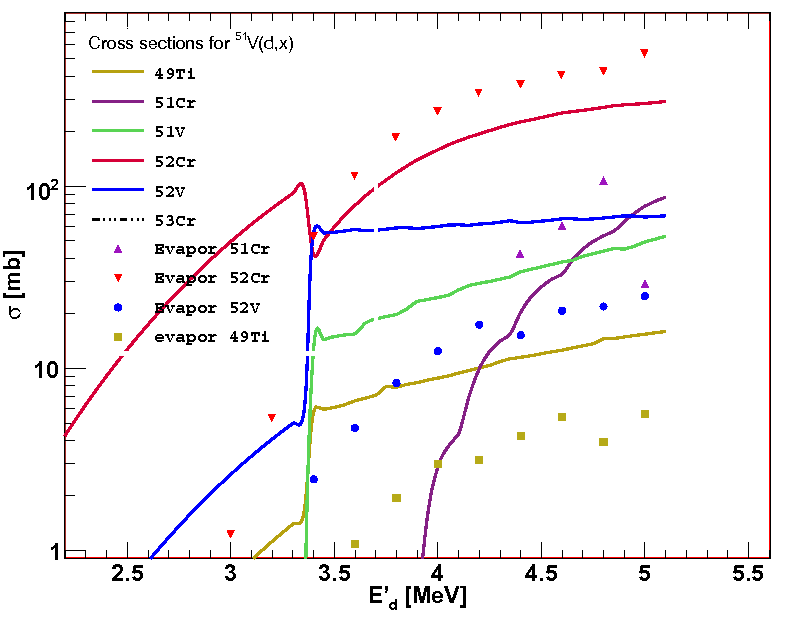
As seen in figure 6.6, large discrepancies were obtained. Below $E_{\mathrm{}}\approx 3.4\mathrm{\;MeV}$ the TALYS and evapOR results are closer. Above 3.4 MeV the cross sections are similar in particular for the $\mathrm{{}^{51}V\left(d,n\right)^{52}Cr}$ reaction.

The target studies were based on the two effects presented in section 5.2.1, due to the neutron distribution and the position of the reaction. Here only results of the study of the reaction $\mathrm{d+^{51}V}$ are presented. The results of the target studies for the $\mathrm{d+^{37}Cl}$ reaction are very similar. In order to study the effect of different neutron emission angles, two events with relatively high and low residual nucleus (${}^{52}\mathrm{Cr}$) kinetic energies were chosen from the evapOR simulation. The energies were $E_{\mathrm{RN1}}=82.4$ MeV and $E_{\mathrm{RN2}}=73.6$ MeV in the laboratory system. The difference is due to the neutron emission angle: the event with energy $E_{\mathrm{RN}1}$ had a large neutron emission angle, $\theta_{\mathrm{n,CM}}^{\mathrm{}}=174.4^{\circ}$ while the event with $E_{\mathrm{RN2}}$ had a small angle, $\theta_{\mathrm{n},\mathrm{CM}}=6.7{}^{\circ}$. The energies $E_{\mathrm{RN1}}$ and $E_{\mathrm{RN2}}$ were used as input to TRIM. The energy losses of the residual nuclei are shown in figure 6.7.

For the two cases the average energy losses are

which gives the velocity

And

which gives the velocity

Next, the effects of this energy-loss difference on the Doppler shifts were studied. In the case of the ${}^{52}\mathrm{Cr}$ residual nucleus, the $\gamma$-ray energy from the $2^{+}$ excited state to the $0^{+}$ ground state is 1434 keV. For detector position at $90^{\mathrm{o}}$relative to the incoming beam and a distance of 15 cm from the target to the front face of the detector, which was chosen for these simulations (see section 6.4), the smallest angle for $\gamma$-ray detection, which corresponds to the largest Doppler shift, is about $70^{\mathrm{o}}$. Thus the difference in $\gamma$ ray energy becomes

which is a small effect. The contribution from the Doppler shift from this studied effect is hence negligible.

The second target effect concerns the position of the reaction. A new TRIM calculation was performed for ${}^{51}\mathrm{V}$ ions with an energy of $E=81.6$ MeV. The energy loss of the ${}^{51}\mathrm{V}$ beam in the target is shown in figure 6.8.

The energy loss of the beam through the target is,

From the previous study of ${}^{52}\mathrm{Cr,}$ the average of $E_{\mathrm{RN1}}$ and $E_{\mathrm{RN2}}$ gives the average energy loss in the case the reactions occur at the beginning of target:

The velocity of the ${}^{52}\mathrm{Cr}$ residual nucleus for the case of a reaction at the end of the target is

and

if the reaction occurs in the beginning of the target. Note that it is assumed that the $\gamma$ rays are emitted after the residual nucleus has exited the target (see section ). The difference in velocities is small and gives a negligible effect on the Doppler shifts at $\theta_{\gamma}=70^{\mathrm{o}}$:

Hence, the position of the reaction in the target can be neglected.

A similar study was done for the $\mathrm{d({}^{37}Cl,n)}$ reaction showing a negligible effect on the Doppler shifts. The average energy loss for the $\mathrm{d({}^{37}Cl,n)}$ reaction was

In figure 6.9, the angular deviation from the beam direction of the ${}^{51}\mathrm{V}$ ions after passing through the $200$ $\mu\mathrm{g/cm^{2}}$ thick Ti target is shown.

The angular distribution of the ions due to straggling has a maximum at $0.1^{\circ}$. This is much smaller than the maximum of the angular distribution due to the neutron emission, see fig. 6.14. Thus, the angular straggling in the target can be neglected.

The compound nucleus has a very short life time compared to the time it takes for it to pass through the target. To prevent the $\gamma$ rays to be emitted while the residual nucleus is still in the target, it is required that the life time are long enough (see section 4). If the $\gamma$ rays are emitted while the residual nucleus still is located inside the target a too large spread of Doppler shift will be the result. The average flight distances of the residual nuclei before emitting the $\gamma$ rays were studied. For the reaction $\mathrm{d({}^{51}V,n)^{52}\mathrm{Cr}}$ the average flight distance $x$, before the emission of the $2^{+}\rightarrow 0^{+}$ $\gamma$-ray in ${}^{52}\mathrm{Cr}$ is

which is an order of magnitude larger than the target thickness $\approx 0.5\mu m$. The life-time of the $2^{+}\rightarrow 0^{+}$ transition in ${}^{38}\mathrm{Ar}$ is 0.578 ps and gives

which is also large compared to the target thickness. Thus the photons will be emitted outside the target material in both reactions.

The effective life time of the transitions of interest must also be shorter than the time it takes for the residual nuclei to travel a distance $\lesssim 1\mathrm{mm}$. This effect was not studied in the present work.

The intrinsic part of the FWHM, $W_{\mathrm{i}}$, given in equation 3.10 is unique for every detector type. This value is used as input to the tracking program MGT. Data from a measurement of the core segment of AGATA crystal number C002 using a ${}^{226}\mathrm{Ra}$ source [34] was used to obtain the energy dependence of $W_{\mathrm{i}}$ for a typical AGATA detector. A straight line was fitted to the data points, see fig. 6.10.

Using the fitted straight line of fig. 6.10, the intrinsic FWHM of the peaks corresponding to the 1434keV and 2168keV $2^{+}\rightarrow 0^{+}$ transitions in ${}^{52}Cr$ and ${}^{38}Ar$ are 2.30keV and 2.83keV, respectively.

Figure 6.11 shows the energy and angular distribution of the neutrons as obtained by evapOR.

The energy distribution (left hand figure) is Maxwellian as expected from equation 2.11. The distribution has a maximum at about 1MeV. According to the plot on the right hand side of figure 6.11, the neutrons have a large emission angle in the laboratory frame. The centroid of the distribution is around $40^{\circ}$.

Figure 6.12 shows the angular distribution of the neutrons in the center of mass system.

Figure 6.13 shows the velocity distribution of the residual nuclei in both reactions. The neutron energy distributions in the laboratory frame are shown in the left panel of figure 6.14. The $\mathrm{d({}^{51}V,n)^{52}Cr}$ reaction contains more neutron events and thus the area under the red histogram is larger. The right panel of figure 6.14 shows the angular distributions of the residual nuclei. There is an evident shift of the angular distribution, implying a smaller mean deflection of the ${}^{52}\mathrm{Cr}$ nuclei compared to the ${}^{38}\mathrm{Ar}$ nuclei. This difference in angular deflection plays a major role in the Doppler shift of the $\gamma$-ray energies.

In figure 6.15 a graphical illustration of the Geant4 simulation is shown. Ten events of the reaction $\mathrm{{}^{51}V\left(77\>MeV\right)+d}$ were generated by evapOR. The direction of motion of the incoming ${}^{51}\mathrm{V}$ beam is from right to left in the figure. For the plot only events belonging to the reaction channel $\mathrm{d({}^{51}V,n)^{52}Cr}$ were selected. Each $\mathrm{{}^{52}Cr}$ residual nucleus emits one $\gamma$ ray, with an energy of 1434 keV, corresponding to the $2^{+}\rightarrow 0^{+}$ transition in ${}^{52}\mathrm{Cr}$.

The $\gamma$ rays were forced to be emitted isotropically into a cone with an opening angle of $20^{\mathrm{o}}$, centered at $90^{\mathrm{o}}$ relative to direction of incoming beam. An AGATA triple cluster detector was placed at that angle, and covered a solid angle which was smaller than the solid angle of the $\gamma$-ray emission cone. The distance between the $\gamma$-ray source and the front of the HPGe crystals was 15 cm in the figure.

Except if otherwise noted, the setup shown in fig. 6.15, with the angle and distance given above, was used in the simulations presented in the following subsections.

As a first simple test, a $\gamma$-ray spectrum was created by summing for each event the total energy deposited in the detector. Such a spectrum is shown in fig. 6.16 for the 2168 keV $\gamma$ ray emitted in the $\mathrm{d({}^{37}Cl,n){}^{38}Ar}$ reaction at $E_{\mathrm{LAB}}\left({}^{37}\mathrm{Cl}\right)=66.5\>\mathrm{MeV}$. The $\gamma$ rays were emitted isotropically into a $90^{\mathrm{o}}\pm 0.5^{\mathrm{o}}$ cone. The intrinsic energy resolution was set to $0$ ($W_{\mathrm{i}}=0$ keV) and no Doppler corrections were applied. The full-energy peak, the single- and double-escape peaks, and Compton background are clearly visible in the spectrum.

Tracked $\gamma$-ray energy spectra were created by feeding the output of the Geant4 simulation into the MGT tracking program. The MGT smearing parameter, which emulates a finite interaction position resolution in the HPGe crystals, was used as one of the parameters in the simulations.

The $\gamma$-ray emission angle, which is needed by the Doppler correction procedure, was calculated by assuming that the $\gamma$ rays were emitted from the center of AGATA and detected at the first interaction point, which was obtained from MGT. For the Doppler correction the velocity vector of the residual nucleus is also needed. Except were otherwise noted, an average value of the velocity vector was used, namely an angle of $0^{\mathrm{o}}$ (motion parallel to the beam) and the average velocity given by the evapOR simulation. The use of such average values is common in fusion-evaporation reactions, when no ancillary detector is available for the event-by-event detection of the velocity vector of the residual nuclei.

Initially, two simulations were performed to verify that the tracking and Doppler correction procedures functioned as expected. In the first simulation, shown in the left panel of fig. 6.17, the 1434 keV $\gamma$ rays from the reaction $\mathrm{d\left({}^{51}V,n\right)^{52}Cr}$, at $E_{\mathrm{LAB}}\left({}^{51}\mathrm{V}\right)=77.0$ MeV, were emitted at an angle of exactly $90^{\mathrm{o}}$ relative to the incoming beam. Gamma-ray tracking with a 5 mm smearing was used, but no Doppler corrections were applied. In the second simulation, shown in the right panel of fig. 6.17, the 1434 keV $\gamma$ rays were emitted isotropically into the $90^{\mathrm{o}}\pm 20^{\mathrm{o}}$ cone covering the solid angle subtended by the triple cluster detector, and both tracking (with 5 mm smearing) and Doppler corrections were applied. The distance from the source to the front of the HPGe crystals was 15.0 cm. The FWHM of the 1434 keV peak in both panels of fig. 6.17 are almost identical, which shows that the $\gamma$-ray tracking and Doppler correction algorithms functioned as expected.

Results of tracked and Doppler corrected $\gamma$-ray spectra from simulations in which also the energy dependence of the intrinsic energy resolution (see section 6.2.4) has been included, are shown for the two reaction in fig. 6.18 and 6.19. The smearing parameter was kept at 5 mm and the $\gamma$ rays were emitted isotropically into the $90^{\mathrm{o}}\pm 20^{\mathrm{o}}$ cone.

Numerical values of the total FWHM $W$ of the peaks in fig. 6.19, and their components (see eq. 3.9) due to the intrinsic resolution ($W_{\mathrm{i}}$ obtained from fig. 6.10) and due to the Doppler effects $W_{\mathrm{D}}$, are given in table 6.1.

The results given in the table clearly show that the contribution to the total FWHM, due to the Doppler effects, is much larger in the reaction $\mathrm{d\left({}^{37}Cl,n\right)^{38}Ar}$ than in the reaction $\mathrm{d\left({}^{51}V,n\right)^{52}Cr}$. The main reason for this is the difference in mass number of the compound nuclei ${}^{38}\mathrm{Ar}$ and ${}^{52}\mathrm{Cr}$. This mass difference leads to a somewhat larger and broader velocity distribution of the residual nuclei (see fig 6.13) and, more importantly, to an angular distribution of the residual nuclei which is both broader and has a maximum at a larger angle (see right panel of fig. 6.14) for the reaction $\mathrm{d\left({}^{37}Cl,n\right)^{38}Ar}$ compared to $\mathrm{d\left({}^{51}V,n\right)^{52}Cr}$. The angular and velocity distributions of the $\gamma$-ray emitting residual nuclei influence directly the Doppler effects, which is seen as an effect on the FWHM of the peaks.

A simulation was also performed by correcting for the Doppler effects introduced by the variation the velocity vector of the residual nucleus. A comparison of the FWHM of the 1434 keV peak obtained when using the average velocity vector and the precise value, as obtained event-by-event from the evapOR simulation, is shown in fig 6.20. For the reaction $\mathrm{d\left({}^{51}V,n\right)}$ at $E_{\mathrm{LAB}}\left({}^{51}\mathrm{V}\right)=77.0$ MeV the FWHM is improved from 4.7 keV to 3.9 keV when the precise value of the velocity vector of the residual nucleus is applied in each event.

A simulation of Doppler effects, following a reaction channel in which $\alpha$ particles are emitted, is shown in fig. 6.21. The emitted $\alpha$ particles are four times heavier than neutrons and have much higher kinetic energies in the laboratory system (compare the left panels of fig. 6.14 and 6.21), which leads to very large spreads both of the energy and angle of the residual nuclei. This in turn leads to very broad $\gamma$-ray peaks, as seen in the right panel of fig. 6.21. Thus, for reaction channels with emission of $\alpha$ particles it is usually necessary to determine event-by-event the velocity vector of the residual nuclei.

Simulations, in which the total FWHM of the 1434 keV and 2168 keV peaks were determined as a function of the MGT smearing parameter, are shown in figures 6.22 and 6.23 for two different detector distances, 15.0 cm and 23.5 cm, respectively. As seen in the figures, the slopes increase for small values of the smearing parameter, up to about 4-8 mm and become more or less constant for larger values. The slopes are quite similar in all cases, although slightly larger for the $\mathrm{d(^{51}V,n)^{52}Cr}$ reaction and for the shorter distance of 15.0 cm.

The interaction position resolution which is expected for the AGATA HPGe crystals is of the order of 5 mm, a value which, however, is not constant. The resolution will depend on the position of the interaction in the crystal. For example in the front part of the crystal, where the electric field is rather non-uniform, the interaction position resolution will be worse compared to a position in the central parts. The interaction position resolution will also depend on the energy deposited in the interaction point. It is expected that it will be proportional to the inverse square root of the interaction energy, a dependence which is implemented in MGT, although not used in this work.

A conclusion of the results shown in fig. 6.22 and 6.23 is that with the proposed reactions, $\mathrm{d(^{37}Cl,n)^{38}Ar}$ at $E_{\mathrm{LAB}}(^{37}\mathrm{Cl})=66.5$ MeV and $\mathrm{d(^{51}V,n)^{52}Cr}$ at $E_{\mathrm{LAB}}(^{51}\mathrm{V})=77.0$ MeV, it will be difficult to get a good determination of the interaction position resolution from the measured FWHM of the peaks. One possibility to improve the sensitive, is to make the measurements for much smaller distances, than what was used in this work (15.0 cm and 23.5 cm). Another possibility is to try to find another reaction with larger average recoil velocities but which still has small enough spread of the residual nucleus velocity vector so that the average Doppler correction procedure may be used.

References

- [1] I. Y. Lee, M. A. Deleplanque, and K. Vetter. Developments in large gamma-ray detector arrays. Reports of Progress in Physics, 66:1095, 2003.
- [2] J. Simpson. The AGATA Project. Journal of physics:Conference Series, 41:72, 2006.
- [3] G. A. Jones. The Properties of Nuclei. Oxford Science Publications, Oxford, 2nd edition, 1987.
- [4] B. Höistad. Lecture notes nuclear physics nv2, 2008.
- [5] G. R. Satchler. Introduction to Nuclear Reactions. The Macmillan press LTD, 1980.
- [6] R. Bock. Heavy Ion Collisions, volume 2. North-Holland, 1980.
- [7] D. G. Swanson and N. T. Porile. Statistical-Model Calculation of the Angular Distributions of (a, n) Reaction Products. Phys. Rev., C1:4, 1970.
- [8] D. W. Lang and K. J. Le Couteur. Pairing energy effects in excited nuclei. Nuclear Physics, 14:21, 1959.
- [9] T. Ericson and V. Strutinsky. On Angular Distributions in Compound Nucleus Processes. Nuclear Physics, 9:689, 1958.
- [10] A. Einstein. On a Heuristic Viewpoint Concerning the Production and Transformation of Light. Annalen der Physik, 17:132, 1905.
- [11] A. H. Compton. A Quantum Theory of the Scattering of X-rays by Light Elements. Phys. Rev., 21:483 , 1923.
- [12] K. S. Krane. Introductory Nuclear physics. Wiley, 3rd edition, 1988.
- [13] H. Bethe. Zur Theorie des Durchgangs schneller Korpuskularstrahlen durch Materie. Annalen der Physik, 397:305, 1930.
- [14] R.P.Feynman. The Feynman lectures on physics, volume 2. ADDISON-WESLEY, 1963.
- [15] G. F. Knoll. Radiation Detection and Measurement. Wiley, 3rd edition, 1999.
- [16] A. Lopez-Martens, et al. Gamma-ray tracking algorithms: a comparison. Nucl. Inst. Meth., A533:454, 2004.
- [17] E. Farnea. Private communication, 2008.
- [18] A. J. Koning, S. Hilaire, and M. C. Duijvestijn. TALYS-1.0. In O. Bersillon, et al. (editors), Proceedings of the International Conference on Nuclear Data for Science and Technology 2007, page 211. EDP Sciences, 2008.
- [19] J. Ziegler and J. Biersack. The Stopping and Range of Ions in Solids. Pergamon Press, New York, 1985.
- [20] J. Beene. Unbublished program evapor, 2008.
- [21] M. Palacz. Private communication, 2008.
- [22] E. Farnea and D. Bazzacco. A Monte Carlo Code for the AGATA Array. In D. R. Napoli, et al. (editors), LNL Annual Report 2003, page 158. 2004.
- [23] S. Agostinelli, et al. Geant4–a simulation toolkit. Nuclear Instruments and Methods in Physics Research A, 506:250, 2003.
- [24] D. Bazacco. Unbublished program mgt, 2008.
- [25] S.Qiang. SubCoulomb Proton Induced Reactions on Copper. Ph.D. thesis, University of Kentucky, 1990.
- [26] M. Sevior, et al. Absolute Cross Sections of Proton Induced Reactions on Cu-65,Ni-64,Cu-63. Australian Journal of Physics, 36:463, 1983.
- [27] D. M. Drake, et al. The Radiative Capture of Fast Protons by Medium-Mass Nuclei. Nuclear Physics, A203:257, 1973.
- [28] Z. E. Switkovski, et al. Threshold Effects in Proton-induced Reactions on Copper. Australian Journal of Physics, 31:253, 1978.
- [29] T. Zhenlan, et al. Excitation Function of Deutron Induced Reactions on Natural Iron. Atomic Energy Science and Technology, 5:506, 1983.
- [30] M. R. Zaman and S. M. Qaim. Excitation functions of (d,n) and (d,a) reactions on high enriched 54Fe: Relevance to the Production of high purity 55Co at a small cyclotron. Radiochimica Acta, 75:59, 1996.
- [31] S. Kailas, et al. V-51(p,n)Cr-51 Reaction from Energy of Protons 1.9 to 4.5 MeV. Pramana, 24:629, 1985.
- [32] J. Zyskind, et al. Competition effects in proton-induced reactions on 51V. Nuclear Physics, A343:295, 1980.
- [33] A. Gadea. Private communication, 2008.
- [34] A. Wiens. Private communication, 2008.