The $\mu\nu$SSM and gravitino dark matter

Supersymmetry (SUSY) is still one of the most attractive theories for physics beyond the Standard Model, and we expect to find its signatures in the forthcoming LHC. However, SUSY has also theoretical problems, and, in particular, a very important one is the so-called $\mu$-problem. This problem arises from the requirement of a SUSY mass term for the Higgs fields in the superpotential of the Minimal Supersymmetric Standard Model (MSSM), $\mu\hat{H}_{u}\hat{H}_{d}$, which must be of the order of the electroweak scale to successfully lead to electroweak symmetry breaking. In the presence of a GUT and/or a gravitational theory with typical scales $10^{16}$ and $10^{19}$ GeV, respectively, one should explain how to obtain a SUSY mass term of the order of $10^{2}-10^{3}$ GeV.

On the other hand, neutrino experiments have confirmed during the last years that neutrinos are massive. As a consequence, all theoretical models must be modified in order to reproduce this result.

The “$\mu$ from $\nu$” Supersymmetric Standard Model ($\mu\nu$SSM) was proposed in the literature [12, 13]¹¹ 1 Several recent papers have studied different aspects of the $\mu\nu$SSM. See the works in [14, 6, 8, 15]. as an alternative to the MSSM. In particular, it provides a solution to the $\mu$-problem and explains the origin of neutrino masses by simply using right-handed neutrino superfields.

The superpotential of the $\mu\nu$SSM contains, in addition to the usual Yukawas for quarks and charged leptons, Yukawas for neutrinos $\hat{H}_{u}\,\hat{L}\,\hat{\nu}^{c}$, terms of the type $\hat{\nu}^{c}\hat{H}_{d}\hat{H}_{u}$ producing an effective $\mu$ term through right-handed sneutrino vacuum expectation values (VEVs), and also terms of the type $\hat{\nu}^{c}\hat{\nu}^{c}\hat{\nu}^{c}$ avoiding the existence of a Goldstone boson and contributing to generate effective Majorana masses for neutrinos at the electroweak scale. Actually, the explicit breaking of R-parity in this model by the above terms produces the mixing of neutralinos with left- and right-handed neutrinos, and as a consequence a generalized matrix of the seesaw type that gives rise at tree level to three light eigenvalues corresponding to neutrino masses [12]. It is worth noticing here that this possibility of using a seesaw at the electroweak scale avoids the introduction of ad-hoc high energy scales in the model.

The breaking of R-parity can easily be understood if we realize that in the limit where neutrino Yukawa couplings are vanishing, the $\hat{\nu}^{c}$ are just ordinary singlet superfields, without any connection with neutrinos, and this model would coincide (although with three instead of one singlet) with the Next-to-Minimal Supersymmetric Standard Model (NMSSM) where R-parity is conserved. Once we switch on the neutrino Yukawas, the fields $\hat{\nu}^{c}$ become right-handed neutrinos, and, as a consequence, R-parity is broken. Indeed this breaking is small because, as mentioned above, we have an electroweak scale seesaw, implying neutrino Yukawas no larger than $10^{-6}$ (like the electron Yukawa) to reproduce the neutrino masses ($\raise 1.29167pt\hbox{$\;<$\kern-7.5pt\raise-4.73611pt\hbox{$\sim\;$}}10^{-2}$ eV).

Since R-parity is broken, one could worry about fast proton decay through the usual baryon and lepton number violating operators of the MSSM. Nevertheless, the choice of $R$-parity is ad hoc. There are other discrete symmetries, like e.g. baryon triality which only forbids the baryon violating operators [4]. Obviously, for all these symmetries R-parity is violated. Besides, in string constructions the matter superfields can be located in different sectors of the compact space or have different extra $U(1)$ charges, in such a way that some operators violating $R$-parity can be forbidden [16], but others can be allowed.

On the other hand, when $R$-parity is broken the lightest supersymmetric particle (LSP) is no longer stable. Thus neutralinos or sneutrinos, with very short lifetimes, are no longer candidates for the dark matter (DM) of the Universe. Nevertheless, if the gravitino is the LSP its decay is suppressed both by the gravitational interaction and by the small R-parity violating coupling, and as a consequence its lifetime can be much longer than the age of the Universe [18]. Thus the gravitino can be in principle a DM candidate in R-parity breaking models. This possibility and its phenomenological consequences were studied mainly in the context of bilinear or trilinear R-parity violation scenarios in [18, 7, 2, 10, 1, 9, 19, 11, 3]. In [2, 1, 9, 11] the prospects for detecting gamma rays from decaying gravitinos in satellite experiments were also analyzed. In a recent work [17] we have discussed these issues, gravitino DM and its possible detection in the FERMI satellite, in the context of the $\mu\nu$SSM. In this talk I will summarize the results obtained in this work.

The superpotential of the $\mu\nu$SSM introduced in [12] is given by

In addition to terms from $L_{soft}$, the tree-level scalar potential receives the $D$ and $F$ term contributions. The final neutral scalar potential can be found in [12, 14]. In the following we will assume for simplicity that all parameters in the potential are real. Once the electroweak symmetry is spontaneously broken, the neutral scalars develop in general the following VEVs:

For our computation below we are interested in the neutral fermion mass matrix. As explained in [12, 14], neutralinos mix with the neutrinos and therefore in a basis where ${\chi^{0}}^{T}=(\tilde{B^{0}},\tilde{W^{0}},\tilde{H_{d}},\tilde{H_{u}},\nu_{R_{i}},\nu_{L_{i}})$, one obtains the following neutral fermion mass terms in the Lagrangian $-\frac{1}{2}(\chi^{0})^{T}\mathcal{M}_{\mathrm{n}}\chi^{0}+\mathrm{c.c.}$, where

with $M$ a $7\times 7$ matrix showing the mixing of neutralinos and right-handed neutrinos, and $m$ a $7\times 3$ matrix representing the mixing of neutralinos and right- and left-handed neutrinos. Both matrices can also be found in [12, 14]. The above $10\times 10$ matrix, Eq. (3), is of the seesaw type giving rise to the neutrino masses which have to be very small. This is the case since the entries of the matrix $M$ are much larger than the ones in the matrix $m$. Notice in this respect that the entries of $M$ are of the order of the electroweak scale while the ones in $m$ are of the order of the Dirac masses for the neutrinos [12, 14].

Concerning the low-energy free parameters of the $\mu\nu$SSM in the neutral scalar sector, using the eight minimization conditions for the scalar potential, one can eliminate the soft masses $m_{H_{d}}$, $m_{H_{u}}$, $m_{\widetilde{L}_{i}}$, and $m_{\widetilde{\nu}_{i}^{c}}$ in favour of the VEVs $v_{d}$, $v_{u}$, $\nu_{i}$, and $\nu^{c}_{i}$. On the other hand, using the Standard Model Higgs VEV, $v\approx 174$ GeV, $\tan\beta$, and $\nu_{i}$, one can determine the SUSY Higgs VEVs, $v_{d}$ and $v_{u}$, through $v^{2}=v_{d}^{2}+v_{u}^{2}+\nu_{i}^{2}$. We thus consider as independent parameters the following set of variables:

where we have assumed for simplicity that there is no intergenerational mixing in the parameters of the model, and that in general they have the same values for the three families: ${\lambda}\equiv{\lambda_{i}}$, $\kappa\equiv{\kappa_{iii}}$, $\nu^{c}\equiv\nu^{c}_{i}$, $A_{\lambda}\equiv A_{\lambda_{i}}$, $A_{\kappa}\equiv A_{\kappa_{iii}}$, $A_{\nu}\equiv A_{\nu_{ii}}$. In the case of neutrino parameters, following the discussion in [15, 14], we need at least two generations with different VEVs and couplings in order to obtain the correct experimental pattern. Thus we have choosen $Y_{\nu_{1}}\neq Y_{\nu_{2}}=Y_{\nu_{3}}$ and $\nu_{1}\neq\nu_{2}=\nu_{3}$.

The soft SUSY-breaking terms, namely gaugino masses, $M_{1,2,3}$, scalar masses, $m_{\tilde{Q},\tilde{u}^{c},\tilde{d}^{c},\tilde{e}^{c}}$, and trilinear parameters, $A_{u,d,e}$, are also taken as free parameters and specified at low scale.

Let us now show that the lifetime of the gravitino LSP is typically much longer than the age of the Universe in the $\mu\nu$SSM, and therefore it can be in principle a candidate for DM. In the supergravity Lagrangian there is an interaction term between the gravitino, the field strength for the photon, and the photino. Since, as discussed above, due to the breaking of R-parity the photino and the left-handed neutrinos are mixed, the gravitino will be able to decay through the interaction term into a photon and a neutrino [18]. Thus one obtains:

where $m_{3/2}$ is the gravitino mass, $M_{P}=2.4\times 10^{18}\,\textrm{GeV}$ is the reduced Planck mass, and $|U_{\widetilde{\gamma}\nu}|^{2}$ determines the photino content of the neutrino

Here $N_{i1}$ ($N_{i2}$) is the Bino (Wino) component of the $i$-neutrino.

The lifetime of the gravitino can then be written as

If $|U_{\widetilde{\gamma}\nu}|^{2}\sim 10^{-16}-10^{-12}$ in order to reproduce neutrino masses, as we will show below, the gravitino will be very long lived as expected (recall that the lifetime of the Universe is about $10^{17}$ s).

For the gravitino to be a good DM candidate we still need to check that it can be present in the right amount to explain the relic density inferred by WMAP, $\Omega_{DM}h^{2}\simeq 0.1$. As it is well known, adjusting the reheating temperature after the inflatinary period of the Universe, one can reproduce the correct relic density for each possible value of the gravitino mass. For example for $m_{3/2}$ of the order of $1-1000$ GeV, as expected from supergravity scenarios, one obtains $\Omega_{3/2}h^{2}\simeq 0.1$ for $T_{R}\sim 10^{8}-10^{11}$ GeV, with gluino masses of order $1$ TeV. It is worth noticing here that even with a high value of $T_{R}$ there is no gravitino problem, since the next-to-LSP decays to standard model particles much earlier than BBN epoch via R-parity breaking interactions.

Let us now show that $|U_{\widetilde{\gamma}\nu}|^{2}\sim 10^{-16}-10^{-12}$ in the $\mu\nu$SSM. We can easily make an estimation [17]. For a $2\times 2$ matrix,

the mixing angle is given by $\tan 2\theta=2c/(a-b)$. In our case (see Eq. (3) and Refs. [12, 14]) $c\sim g_{1}\nu\sim 10^{-4}$ GeV (represents the mixing of Bino and left handed neutrino), $a\sim 1$ TeV (represents the Bino mass $M_{1}$), and $b=0$. Thus one obtains $\tan 2\theta\sim 10^{-7}$, implying $\sin\theta\sim\theta\sim 10^{-7}$. This gives $|U_{\widetilde{\gamma}\nu}|^{2}\sim 10^{-14}$. More general, $\theta\sim\frac{g_{1}\nu}{M_{1}}\sim 10^{-6}-10^{-8}$, giving rise to

We have carried out the numerical analysis of the whole parameter space discussed in Sect. 2, and the results confirm this estimation [17].

Since in R-parity breaking models the gravitino decays producing a monochromatic photon with an energy $m_{3/2}/2$, one can try to extract constraints on the parameter space from gamma-ray observations [18]. Actually, model independent constraints on late DM decays using the gamma rays were studied in [20].

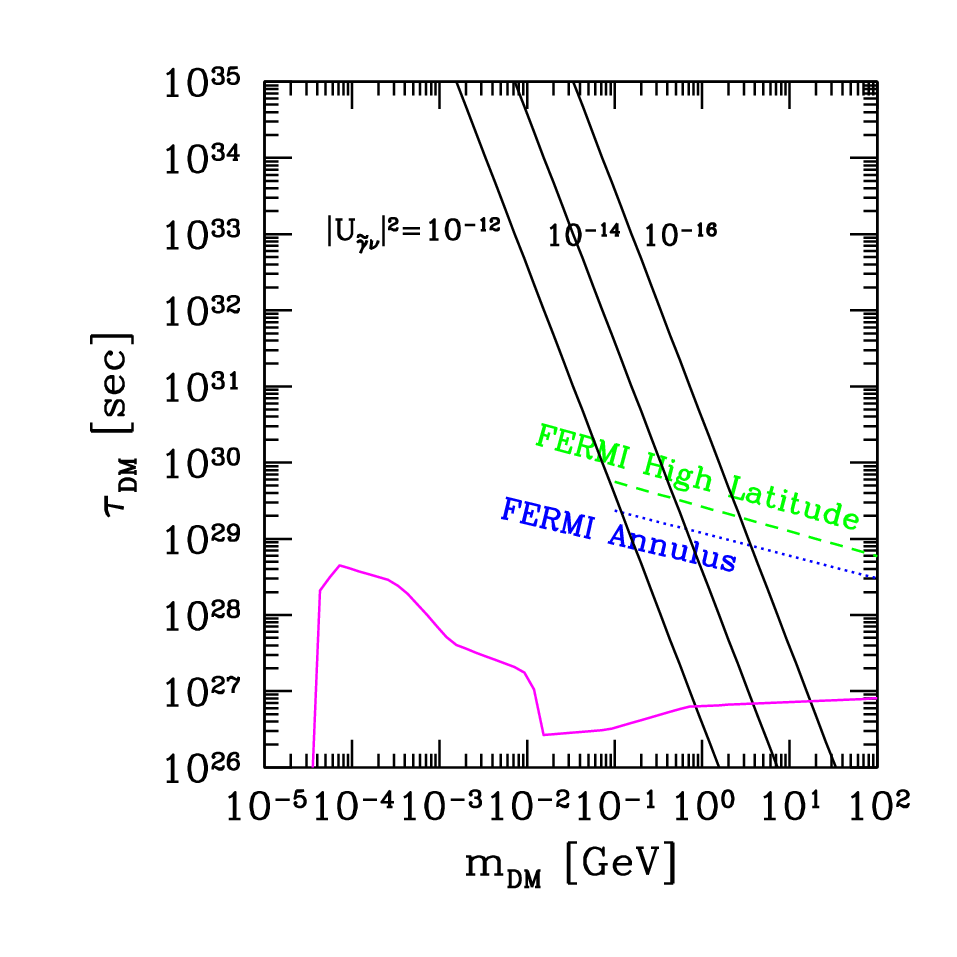There, the decaying DM was constrained using the gamma-ray line emission limits from the galactic center region obtained with the SPI spectrometer on INTEGRAL satellite, and the isotropic diffuse photon background as determined from SPI, COMPTEL and EGRET data. These constraints are shown in Fig. 1 (from Ref. [17]), where the region below the magenta line is excluded. A conservative non-singular profile at the galactic center is used.

On the other hand, the FERMI satellite [5] launched in June 2008 is able to measure gamma rays with energies between 0.1 and 300 GeV. We also show in Fig. 1 the detectability of FERMI in the ’annulus’ and ’high latitude’ regions following the work in [1]. Below the lines, FERMI will be able to detect the signal from decaying DM. Obviously, no signal means that the region would be excluded and FERMI would have been used to constrain the decay of DM [1].

Finally, we show in the figure with black solid lines the values of the parameters predicted by the $\mu\nu$SSM using Eq. (7), for several representative values of $|U_{\widetilde{\gamma}\nu}|^{2}$ discussed in Eq. (9). We can see that values of the gravitino mass larger than 20 GeV are disfavored in this model by the isotropic diffuse photon background observations (magenta line). In addition, FERMI will be able to check important regions of the parameter space with gravitino mass between $0.1-20$ GeV and $|U_{\widetilde{\gamma}\nu}|^{2}=10^{-16}-10^{-12}$ (those below the green line).

Let us now discuss in more detail [17] what kind of signal is expected to be observed by FERMI if the gravitino lifetime and mass in the $\mu\nu$SSM (black solid lines) correspond to a point below the green line in Fig. 1

As it is well known, there are two sources for a diffuse background from DM decay. One is the cosmological diffuse gamma ray coming from extragalactic regions, and the other is the one coming from the halo of our galaxy.

The photons from cosmological distances are red-shifted during their journey to the observer and the isotropic extragalactic flux can be found in [18, 1]. On the other hand, the photon flux from the galactic halo shows an anisotropic sharp line. For decaying DM this is given by

where the halo DM density is integrated along the line of sight, and we will use a NFW profile, $\rho_{NFW}(r)=\frac{\rho_{h}}{r/r_{c}(1+r/r_{c})^{2}}$, where we take $\rho_{h}=0.33\,\textrm{GeV}/\,\textrm{cm}^{3}$, $r_{c}=20$ kpc, and $r$ is the distance from the center of the galaxy. The latter can be re-expressed using the distance from the Sun, $s$, in units of ${R_{\odot}}=8.5$ kpc (the distance between the Sun and the galactic center) and the galactic coordinates, the longitude, $l$, and the latitude, $b$, as $r^{2}(s,b,l)={R_{\odot}}^{2}[(s-\cos b\cos l)^{2}+(1-\cos^{2}b\cos^{2}l)]$.

As an example, let us compute with these formulae the expected diffuse gamma-ray emission in the mid-latitude range ($10^{\,\circ}\leq|b|\leq 20^{\,\circ}$), which is being analized by FERMI, for the case of gravitino DM. Let us assume for instance a value of $m_{3/2}=3.5$ GeV and $\left|U_{\tilde{\gamma}\nu}\right|^{2}=8.8\times 10^{-15}\,(1.7\times 10^{-15})$ in the $\mu\nu$SSM, corresponding to $\tau_{3/2}=10^{27}$ ($5\times 10^{27}$) s, using Fig. 1. We convolve the signal with a Gaussian distribution with the energy resolution $\Delta E/E=0.09$, between $E=1-10\,\textrm{GeV}$, following [5], and then we average the halo signal over the region for the mid-latitude range mentioned above.

The results for the two examples are shown in Fig. 2, where the green dashed line corresponds to the diffuse extragalactic gamma ray flux, the magenta solid line corresponds to the gamma-ray flux from the halo, and the black solid lines represent the conventional background. The total gamma-ray flux, including background, extragalactic, and line signal, is shown with red solid lines. We can see that the sharp line signal associated to an energy half of the gravitino mass, dominates the extragalactic signal and can be a direct measurement (or exclusion) in the FERMI gamma ray observation.