Quantum Adiabatic Algorithms, Small Gaps, and Different Paths
Abstract
We construct a set of instances of 3SAT which are not solved efficiently using the simplest quantum adiabatic algorithm. These instances are obtained by picking random clauses all consistent with two disparate planted solutions and then penalizing one of them with a single additional clause. We argue that by randomly modifying the beginning Hamiltonian, one obtains (with substantial probability) an adiabatic path that removes this difficulty. This suggests that the quantum adiabatic algorithm should in general be run on each instance with many different random paths leading to the problem Hamiltonian. We do not know whether this trick will help for a random instance of 3SAT (as opposed to an instance from the particular set we consider), especially if the instance has an exponential number of disparate assignments that violate few clauses. We use a continuous imaginary time Quantum Monte Carlo algorithm in a novel way to numerically investigate the ground state as well as the first excited state of our system. Our arguments are supplemented by Quantum Monte Carlo data from simulations with up to 150 spins.
I Introduction
Quantum adiabatic algorithms are designed for classical combinatorial optimization problems [8]. In the simplest case, such algorithms work by adiabatically evolving in the ground state of a system with Hamiltonian that is a function of a parameter which is increased from to as a function of time. is called the beginning Hamiltonian and , which is instance dependent, is called the problem Hamiltonian. The minimum (for ) eigenvalue gap between the ground state and first excited state of is related to the runtime of the adiabatic algorithm. If has an exponentially small minimum gap then the corresponding algorithm is inefficient, whereas a minimum gap which scales inverse polynomially corresponds to an efficient quantum adiabatic algorithm.
Whether or not quantum adiabatic algorithms can be used to solve classically difficult optimization problems efficiently remains to be seen. Some numerical studies have examined the quantum adiabatic algorithm on random sets of instances of optimization problems where these sets are thought to be difficult for classical algorithms. These studies have reported polynomial scaling of the minimum gap out to about bits [6, 20, 12]. Whether this scaling persists at high bit number has recently been called into question [21]. Meanwhile there has been no rigorous analytical result that characterizes the performance of the quantum adiabatic algorithms on random instances of NP-complete problems.
Over the years there have been a number of proposed examples which were meant to demonstrate failures of the adiabatic algorithm on specific problems. In reference [18], van Dam et al constructed examples intended to foil the adiabatic algorithm, but these examples used a nonlocal cost function. Related 3SAT examples of van Dam and Vazirani [19] indeed cannot be solved efficiently using the quantum adiabatic algorithm. However it was shown in [5] that such 3SAT instances do not pose a problem for the quantum adiabatic algorithm if, having fixed a specific problem Hamiltonian, one randomly chooses multiple interpolating paths between the initial and final Hamiltonians and runs the adiabatic algorithm once for each random path. Fisher [9] has constructed an interesting but specialized example on which the quantum adiabatic algorithm is inefficient. (A later example of Reichardt [17] is based on this.) We do not know if random path change helps here. (It is interesting to note that in this case the runtime scales like where is the number of bits.) The authors of reference [22] pointed out that a certain adiabatic algorithm for 3SAT is not efficient. However, this was due to a perverse and avoidable nonlocal choice of beginning Hamiltonian [7].
One purpose of this paper is to discuss a different type of challenge to adiabatic optimization which has recently come to light. (See references [3, 4, 2] and in a different context [15].) It seems to us that in the history of challenges to adiabatic optimization, this may be the most serious. The takeaway message of this work is that a small minimum gap for can arise when the Hamiltonian has features which are seen in the following construction. First suppose that we start with a problem Hamiltonian which has two degenerate ground states and corresponding to bit strings of length that differ in order bits. We then expect that the two lowest eigenvalues of will look something like figure 1. Note that one curve is always below the other except at even though in the figure they appear to meld because they have the same slope at . Suppose that the upper curve (the first excited state for near ) approaches the state and the lower curve approaches the state as We now form the problem Hamiltonian , where is a term that penalizes the state but not the state Then, for the two lowest eigenvalues of , we expect to have the situation pictured in figure 2, where there is a small gap near .


In this paper we discuss a simple way of generating random instances of 3SAT where the corresponding adiabatic Hamiltonian has the difficulty discussed above. We argue in section III that this problem can be overcome (for the set of instances we consider) by randomizing the choice of beginning Hamiltonian.
We present a continuous imaginary time Quantum Monte Carlo algorithm, which is a modification of the Heat Bath algorithm of Krzakala et al [14]. (“Quantum Monte Carlo” is a completely classical numerical technique for finding properties of quantum systems and is not a quantum algorithm.) We use this numerical technique in a novel manner which allows us to investigate both the ground state and the first excited state of our Hamiltonian and thereby detect the presence or absence of a small gap between them. This differs from the standard application of the Quantum Monte Carlo method in that we are able to obtain information about the first excited state using a simple procedure which we have validated at low bit number by comparing our results to exact numerical diagonalization. These Quantum Monte Carlo simulations support our claim that the problem we describe can be overcome using random path change.
II Problematic Instances
We now describe the method we use to generate bit random instances of 3SAT that lead to quantum adiabatic Hamiltonians with small minimum gaps. To do this we first generate an instance with exactly two satisfying assignments given by the bit strings and . Each clause of the 3SAT instance specifies a subset of 3 bits and a particular assignment to those three bits which is disallowed. In order to only generate instances which are consistent with the bit strings and , we only use clauses for which
We add such clauses one at a time uniformly at random and stop as soon as these two bit strings are the only bit strings which satisfy all of the clauses that have been added. (In practice to check whether or not this is the case we use a classical 3SAT solver.) We write for the total number of clauses in the instance. We note that the number of clauses obtained using this procedure scales like . We need this many clauses in order to ensure that each bit is involved in some clause. On the other hand, when the number of clauses is the probability of additional satisfying assignments goes to zero as .
We now consider the problem Hamiltonian corresponding to this instance, which we define to be
Each term in this sum is if violates the clause and otherwise. For the beginning Hamiltonian we choose
| (1) |
The two lowest eigenvalues of the Hamiltonian will then both approach as , as in figure 1. The ground state for values of which are sufficiently close to 1 will approach either or as . Suppose for values of close to the state that approaches has lowest energy. Then we add an extra term which acts on bits and and which penalizes this state but not
and pick
(Note that this extra term has a multiplicative factor of , to avoid any degeneracy of the first excited state at .) In the case where the lowest energy state near approaches we instead add
The Hamiltonian is then expected to have a small gap near as depicted in figure 2. We expect the location of the minimum gap to approach as .
Location of the Minimum Gap
In order to determine the dependence of the location of the avoided crossing on the number of spins and the number of clauses , we consider the perturbative corrections to the energies of the states and around . We will show that the low order terms in the perturbation series reliably predict a crossing at11 1 The notation means that, for sufficiently large, for some constants and . .
With the Hamiltonian constructed in the previous section, one of these states has energy at (call this the lower state ) and the other state has energy at (we call this the upper state ). We write our Hamiltonian as
| (2) |
and we then consider the term as a perturbation to expanding around .
To understand why we trust perturbation theory to predict the location of the near crossing, consider a system which is composed of two disconnected sectors, and , so the corresponding Hamiltonian is of the form
In this situation the generic rule that levels do not cross does not apply and we can easily imagine that the two lowest levels look like what we show in figure 3, where the levels actually cross at .

Imagine that low order perturbation theory around can be used to get good approximations to the ground state energies of and for near , even for somewhat to the left of Then it is possible to accurately predict . Our situation is very close to this. We can think of as consisting of the states close to in Hamming weight, and as states close to in Hamming weight. Similarly, we view and as the restrictions of to these sectors. Note that it takes powers of the perturbation to connect and and this is why we view and as essentially disconnected.
Although figure 3 looks like figure 2, it is figure 2 that depicts the actual situation, where the two levels avoid crossing. This true near cross means that the perturbation series in the actual theory will diverge very close to . However this divergence will only be seen at high order, in fact at an order which is proportional to . The low order terms of the perturbation series in figure 3 are the same as the low order terms of the perturbation series in figure 2, so we can trust low order perturbation theory to locate .
(We argue below that as a function of the number of bits, , goes to as goes to infinity. This implies that the radius of convergence of the perturbation theory for the full , expanded about , goes to as goes to infinity. This fact has no bearing on our argument that low order perturbation theory can be used to accurately predict
For small values of the parameter , the energies of the two states under consideration can be expanded as
| (3) | |||||
| (4) |
It is easy to see that each expansion (inside the square brackets) only contains even powers. Note that is guaranteed to be negative as is always the case for 2nd order perturbation theory of the ground state. In addition, since we added a term to penalize the state which had smaller energy near before adding the clause, we expect that . We are interested in the behaviour of the difference for randomly generated instances (as generated using the prescription of the previous section) as a function of the number of spins in the limit . This requires us to further investigate the behaviour of each coefficient and as a function of and .
In fact to locate we need only to go to second order in perturbation theory. From equation 2 we view as the unperturbed Hamiltonian, and as the perturbation, with as the expansion parameter. Now so at second order we get
Similarly,
where the in the denominator is
The expected energy penalty incurred when flipping a bit of either or is of order since each bit is typically involved in clauses. So the coefficients and are of order since the energy denominators involved are . We now show that their difference is of order . Write
where for each ,
| (5) |
Recall that where is the penalty term from the final clause which acts only on the first 3 bits. Therefore, for
Our procedure for generating instances is symmetric between the strings and so averaging over instances it is clear that the mean of for is . Thus we expect to be (approximately) Gaussian with mean and standard deviation proportional to , where is the standard deviation of each for . To compute we note that
Again using the symmetry between all zeros and all ones, we conclude that the numerator is of order and the denominator is of order . Hence we expect to be . So is of order We will now locate using second order perturbation theory and afterwards argue that higher orders do not change the result. Returning to equations 3 and 4, equating the two energies at second order we have
so
| (6) |
The 4th order correction to the energy of the lower state is given by
where
and . Writing , this can be expressed as
Now consider the terms in this expression corresponding to indices for which and the bits and do not appear in a clause together. Under these conditions we have
So we can write
| (7) | |||||
Here the subscript “clausemates” indicates that we sum only over pairs of indices which appear together in at least one clause of the 3SAT instance corresponding to . For , since the unperturbed energy is we obtain
| (8) | |||||
Let’s look at the first sum in each of equations 7 and 8 where goes from to . Each term as goes from to is of order and so the difference of the two sums is . The second sums (those which are restricted to clausemates) contain of order terms. Each denominator is of order and the numerators are since the only contribution to the numerator is from clauses in which involve bits and together. Separating out the terms where and/or are or , we conclude that the contribution to from the clausemate terms is . For our instance generation grows like so this clausemate contribution is asymptotically dominated by the first term which scales like . So the fourth order contribution to the difference of energies is . At which we determined at second order to be , the fourth order contribution to the energy difference is . The fourth order corrections can therefore be neglected in determining the location of Sixth order and higher contributions to the difference are even smaller.
III Fixing the Problem by Path Change
In our instance generation we manufactured a small gap by penalizing the planted assignment corresponding to the energy eigenstate with the smallest energy near . Since the slopes of the two curves in figure 1 are the same at , the second derivatives determine which eigenvalue is smaller near . After penalization we have which is consistent with the near crossing in figure 2. Suppose instead that we penalize the assignment corresponding to larger energy in figure 1. Then we expect the situation depicted in figure 4 where no level crossing is induced.
We imagine that the instances that we manufacture with a small gap as in figure 2 are a model for what might be encountered in running the quantum adiabatic algorithm on some instance a quantum computer is actually trying to solve. There is a strategy for overcoming this problem. The idea is to produce figure 4, with reasonable probability, by randomly modifying the adiabatic path which ends at , of course making no use of the properties of the particular instance. For this purpose one could use any random ensemble of paths such that and the ground state of is simple to prepare. However in this paper we only consider randomly changing the beginning Hamiltonian. We have made this choice so that we are able to use our Quantum Monte Carlo method to numerically verify our arguments. Like other Quantum Monte Carlo methods, the method we use does not work when the Hamiltonian has nonzero off-diagonal matrix elements with positive sign.
Starting with an instance where has a tiny gap due to the problem discussed above, we now consider a different adiabatic path obtained by keeping the same problem Hamiltonian but choosing a different beginning Hamiltonian in a random fashion which we will prescribe below. We argue that the small gap near is then removed with substantial probability, so that by repeating this procedure a constant number of times it is possible to find an adiabatic path without a small gap near .

The way that we choose a random Hamiltonian is to first draw random variables for , where each is chosen to be or with equal probability. We then take
| (9) |
We write and for the analogous quantities to and for the new Hamiltonian . The point is that by randomizing in the way we prescribe, there is a substantial probability that one will obtain , and in that case one expects no avoided crossing near Write
where the are fixed by the instance (and are defined in equation 5). Since we have fixed the problem Hamiltonian , the only random variables appearing in the above equation are the . We have so the mean value of is then
But more importantly
The variance of this difference is
which is . For a fixed instance with a corresponding fixed set the random variable is approximately Gaussian and from its mean and variance we see that the probability that is positive and in fact greater than , for , is bounded away from independent of . This means that there is a good chance that randomizing turns the situation depicted in figure 2 into the situation depicted in figure 4.
In the case of two planted satisfying assignments with one penalized to produce a small gap when the beginning Hamiltonian is of equation 1, we have shown that a random choice for the beginning Hamiltonian of equation 9 can with substantial probability remove the small gap. This gives further weight to the idea that when running the quantum adiabatic algorithm on a single instance of some optimization problem, the programmer should run the quantum adiabatic algorithm repeatedly with different paths ending at [5].
What if there are satisfying assignments and all but one are penalized?
We have considered instances of 3SAT for which the corresponding problem Hamiltonian has a unique ground state and a nondegenerate first excited state that is far from the ground state in Hamming weight. In this case we have shown that the path change strategy succeeds in removing a tiny gap. What happens when we have mutually disparate solutions and we penalize all but one of them? We show (under some assumptions) that for large , path change will succeed after a number of tries polynomial in . We can therefore hope for success if there are disparate assignments which violate few clauses and scales polynomially with . On the other hand when is superpolynomial in we have no reason to be optimistic about the performance of the quantum adiabatic algorithm.
The energies for of the states under consideration can be expanded as in equations 3 and 4. Write for the second order corrections in these expansions. If we add a small number of clauses to this instance which penalize all the solutions except for a randomly chosen one which we call (forming a new problem Hamiltonian ) then the differences will not change substantially. So we are interested in the differences
where
| (10) |
and where are the ground states of . The adiabatic algorithm applied to this instance with problem Hamiltonian will succeed if all of the above differences are positive, for There is a chance of this occurring. If they are not all positive, then we have encountered an instance which we expect to have a small gap. In this case, we randomize the beginning Hamiltonian as in the previous subsection. This produces new values for the second order energy corrections and the relevant differences are given by
| (11) |
where the random variables are or with equal probability (and the are fixed). With this fixed problem Hamiltonian, how many times do we have to randomize the beginning Hamiltonian (by drawing a random set ) to produce algorithmic success? For large , the random variables are approximately jointly Gaussian with expectation and variance given by
The correlation (the covariance divided by the product of the standard deviations) between any two of these random variables is given by
| (12) |
We now argue that the above correlation is typically equal to when is large. To see this, we can expand the above expression using equation 10. We imagine that the instances have been generated so that the law of large numbers applies and that in the limit of large n the quantity
approaches an independent value and the quantity
approaches a value independent of and for . Using this in equation 12, we obtain that the correlation is equal to (for and in the limit of large ).
Recall that the problem Hamiltonian has been fixed and therefore the are set. We have argued that for large n the differences have approximately a joint normal distribution with pairwise correlations equal to The probability that a random choice of the make the algorithm succeed is
Note that in the last line we have subtracted the mean and divided by the standard deviation. Using a standard trick we can rewrite the above probability as (in the limit of large n),
| (13) |
where and are independent normal random variables with mean zero and variance . This follows from the fact that the joint normal distribution is specified by its marginal distributions and pairwise correlations. Essentially and are the (normalized) changes in the quantities and provided by the randomization.
At this point, in order to evaluate equation 13 we need to understand the magnitude of the RHS of the inequality. Consider typical values for the sum . As in section II we assume that this sum is Gaussian in the limit of large with mean and standard deviation approximated by .
(In the argument below, we use some properties of the Gaussian distribution which follow from the inequalities
For the approximately Gaussian random variables with mean and variance , for some constant it will hold with high probability (in the limit of large ) that
Now the random variable satisfies with probability which is only polynomially small in . For each the probability that is polynomially small in and we use the bound
The first term on the RHS is only polynomially small, and each of the terms in the product are at least if is large enough. So the probability that the adiabatic algorithm succeeds is at worst polynomially small in . By repeating the randomization a polynomial number of times we expect to succeed with high probability.
IV Quantum Monte Carlo and Numerical Results
Continuous Imaginary Time Quantum Monte Carlo
This section is a review of continous imaginary time Quantum Monte Carlo (which is a classical path integral simulation technique for extracting properties of quantum systems [16]). In particular we will show how this method can be used to compute thermal expectation values of Hermitian operators at inverse temperature . We start with a Hamiltonian H which we write as
where is diagonal in some known basis , and V is purely off diagonal in this basis. We require that all the nonzero matrix elements of are negative. For the Hamiltonian with as in equation 1, we have
Here we include the factor of in the definition of since we are not doing perturbation theory in this quantity.
The partition function can be expanded using the Dyson series as follows
Here we use the notation . We can then insert complete sets of states and take the trace to obtain the path integral
| (14) | ||||
In this formula we have used the notation , where the function is defined by
So in particular
We view the function as a path in imaginary time which begins at and ends at Then equation 14 is a sum over paths, where every path is assigned a positive weight according to a measure
Note that the fact that is positive semidefinite follows from our assumption that all matrix elements of are negative. We write
| (15) |
for the normalized distribution over paths.
We now discuss how one can obtain properties of the quantum system as expectation values with respect to the classical measure We are interested in ground state properties, but in practice we select a large value of and compute thermal expectation values at this inverse temperature. If is sufficiently large then these expectation values will agree with the corresponding expectation values in the ground state. It is straightforward to show that for any operator which is diagonal in the basis, the thermal expectation value can be written as
| (16) |
where The notation means average with respect to the classical probability distribution over paths.
This immediately allows us to estimate quantities such as the diagonal part of the Hamiltonian
| (17) |
Another quantity that we find useful in our study is the Hamming weight operator defined by
| (18) |
which can also be estimated using equation 16. In order to estimate the thermal expectation value of the full Hamiltonian we use equation 17 as well as the expression
| (19) |
where is the number of transitions in the path. (Equation 19 is not as simple to derive as equation 16.) So by generating paths from the distribution and then computing averages with respect to , we can evaluate the thermal expectation value of the energy at a given inverse temperature and by taking sufficiently large we can approximate the ground state energy.
Generating paths from the distribution is itself a challenging task. We use a modified version of the heat bath algorithm of Krzakala et al [14] which we describe in the appendix. As with other Quantum Monte Carlo methods, this algorithm is a Markov Chain Monte Carlo method. In order to sample from the distribution , one defines a Markov Chain over the state space consisting of all paths, where the limiting distribution of the chain is . To obtain samples from one starts in an initial path and then applies some number of iterations of the Markov Chain. If is sufficiently large then the distribution of the paths found by further iteration will be close to We use these subsequent paths to compute averages with respect to .
Equilibration of the Quantum Monte Carlo and Identification of Level Crossings
The discussion in the previous section demonstrates how one can estimate expectation values of various quantities in the ground state of a quantum system. The method is “continuous time” so there is no discretization error and for fixed quantities can be arbitrarily well approximated with enough statistics. We use the Quantum Monte Carlo method in a nonstandard way in order to be able to study the lowest two eigenstates of our Hamiltonian (as opposed to just the ground state).
As described in the previous section, the standard procedure for generating configurations is to equilibrate to the distribution from some initial path (we call this the seeded path) by applying the Monte Carlo update times. In order to ensure that one has equilibrated after Monte Carlo updates, one could for example do simulations with two or more different initial paths (seeded paths) and check that the values of Monte Carlo observables appear to converge to the same seed independent values.
For each instance we consider, we run two different Monte Carlo simulations that are seeded with two different paths and . These seeds are paths with no flips in them, corresponding to the two states and ,
With each seed, we run the Monte Carlo simulation for some total number of Monte Carlo sweeps, taking data every sweeps. Here a single sweep is defined to be iterations of our Monte Carlo update rule as described in the appendix (where is the number of spins). We then remove the first Monte Carlo samples, and use the remaining Monte Carlo samples to estimate the thermal averages
In order to convince the reader that the Monte Carlo algorithm works correctly, and that we can obtain information about the first excited state, we show data at 16 bits where exact numerical diagonalization is possible. In figures 5 and 6 we show the result of this procedure for a 3SAT instance with 16 bits, with problem Hamiltonian (before adding the penalty term , so that the levels are degenerate at ). This instance has 122 clauses. The inverse temperature is . The total number of Monte Carlo sweeps at each value of is , with data taken after every fifth sweep (this gave us data samples). We use samples solely for equilibration at each value of . Note that the Monte Carlo simulations with the two different seeds (corresponding to the circles and crosses in the figures) only agree for values of less than roughly . We interpret this to mean that at these values of the Quantum Monte Carlo has equilibrated to the proper limiting distribution regardless of the seed. As increases past , the two simulations abruptly begin to give different results. In this case the simulation seeded with finds a metastable equilibrium of the Markov Chain (i.e not the limiting distribution ), which corresponds in this case to the first excited state of the Hamiltonian. For above we can see from the comparison with exact diagonalization that the two differently seeded values allow us to compute the energies (figure 5) and Hamming weights (figure 6) of the lowest two energy levels of our Hamiltonian.
What is happening here is that for large , the quantum system can be thought of as consisting of two disconnected sectors. One sector consists of states in the z basis with low Hamming weight and the other with Hamming weight near . The Quantum Monte Carlo “equilibrates” in each sector depending on the initial seed as can be seen by the smooth data in each sector. (Note that data is taken independently at each value of s.) The lower of the cross and circle at each value of in figure 5 is the ground state energy. Of course if the classical algorithm ran for long enough then the circles in figure 5 would lie on the crosses for every value of .
In figures 7 and 8 we show data taken for the same instance after the penalty clause is added that removes the degeneracy at . In this case the two levels have an avoided crossing as expected and which can be seen by exact numerical diagonalization in figure 7. However in the Monte Carlo simulation with two seeds there are two essentially disconnected sectors and the two levels being tracked do cross. When we see this behaviour in the Monte Carlo simulation, we interpret it as compelling evidence that there is a tiny gap in the actual system, which occurs where the curves cross. In figure 8 first look at the curves coming from the exact numerical diagonalization. The Hamming weight of the ground state decreases and then abruptly rises at the location of the minimum gap. The Hamming weight of the first excited state also undergoes an abrupt change at the location of the minimum gap. Not surprisingly the exact diagonalization clearly shows the behaviour we expect with the manufactured tiny gap. Now look at the Monte Carlo data which is interpreted by first looking at figure 7. In figure 7 the true ground state is always the lower of the circles and the crosses. For below it is the crosses and for larger than it is the circles. Accordingly in figure 8 the Hamming weight of the ground state is tracked by the crosses for below and by the circles for above . We can therefore conclude, based only on the Monte Carlo data, that the Hamming weight of the ground state changes abruptly. At higher bit number we do not have exact numerical diagonalization available but we can still use the Quantum Monte Carlo to extract key information.
Randomizing the Beginning Hamiltonian
For the 16 spin Hamiltonian depicted above, we now consider randomizing the beginning Hamiltonian as described in section III. In order to minimize the number of times we run the Monte Carlo algorithm (this will be more of an issue at high bit number where simulations are very time consuming), we generated many different sets of coefficients and calculated the differences with fixed problem Hamiltonian and beginning Hamiltonians
According to our discussion in section III, we expect the avoided crossing near to be removed for choices of coefficients such that the difference . We made a histogram of the (shown in figure 9) and randomly chose three sets of coefficients such that for each. Our analysis predicts that in these cases the crossing will be removed. As expected, each of these three sets of coefficients resulted in an adiabatic Hamiltonian with the small gap removed, although in one there was another small gap at a smaller value of . We plot the Monte Carlo data for one of these sets in figures 10 and 11.
In section II we argued that we could manufacture a small gap in a 3SAT instance as sketched in figure 2. Our 16 bit instance is a concrete example of this and the tiny gap can be seen in figure 7. In section III we argued that by randomizing the beginning Hamiltonian we should be able to produce figure 4. This is what we see concretely at 16 bits in figure 10. We now tell the same story at 150 bits using only Monte Carlo data since exact numerical diagonalization is not possible.
Data for an Instance of 3SAT with 150 bits
In addition to validating our method at 16 bits, we studied 3SAT instances with and bits using our Quantum Monte Carlo simulator. The data from these simulations for the most part supported our arguments. In this section we present Monte Carlo data taken for a double plant instance of 3SAT with 150 spins and 1783 clauses. In this case the inverse temperature , and the total number of Monte Carlo sweeps at each value of is , with data taken every fifth sweep (giving data samples). The first data samples at each value of are removed for equilibration. We ran our simulations on a 648 processor SiCortex computer cluster in embarrassingly parallel fashion. We used a different processor for each value of and each value of the seed. Data taken at the lower values of took the longest to accumulate, in some cases more than 10 days on a single processor for a single data point.
Figures 12 and 13 show the energy and the Hamming weight before the penalty clause is added, running with two different seeds. In figure 12 for large values of , the crosses are always below the circles and track the ground state which ends at as can be seen in figure 13. We have also plotted the second order perturbation theory energies for these two levels, expanding around . Note the good agreement between the second order perturbation theory and the Monte Carlo data all the way down to .
Since the lower curve corresponds to , we penalize this assignment by the addition of a single clause to form attempting to manufacture a near crossing. In figure 14, the circle data is below the cross data for near but the two curves cross near . This is seen clearly in figure 15 where the energy difference is plotted. From the Monte Carlo data we conclude that has a tiny gap. The location of the avoided crossing is well predicted by second order perturbation theory as can be seen in figure 15.
The Monte Carlo data at 150 bits shows that we can make an instance of 3SAT with a tiny gap following the procedure outlined in section II. We now use the Monte Carlo simulator to show that a randomly chosen can alter the Hamiltonian so that this small gap becomes large. For the instance at hand we first compute the difference for randomly chosen sets of coefficients. The histogram of these differences is plotted in figure 17. After doing this we randomly selected (from this set) two sets of coefficients such that . For both of these sets of coefficients we saw that the crossing at was no longer present, although in one case there appeared to be a new crossing at a much lower value of . Figures 18 and 19 show the Monte Carlo data for the choice of which does not appear to have any crossing. At 150 bits we see compelling evidence that the story outlined in sections II and III is true.
Is near ?
We argued that should go to for large enough . However our 16 bit example has and the 150 bit example has . Recall from equation 6 that . At 16 bits with we have and at 150 bits with we have . Although asymptotically is of order , for these values of we are not yet in the regime where .
Even though is not near 1 for our instance at 150 bits, we see from figure 15 that second order perturbation theory can be used to predict the location of . This is because the fourth order contribution to the energy difference is quite small. So already at 150 bits we can predict the presence or absence of an avoided crossing using second order perturbation theory.
V Conclusions
We have introduced a new Quantum Monte Carlo technique to analyze the performance of quantum adiabatic algorithms for instances of satisfiability. Using seeded configurations (in the Monte Carlo simulation) corresponding to disparate low lying states, our technique exposed the presence or absence of an exponentially small gap without ever actually computing the gap.
We used this method to numerically investigate a set of random instances of 3SAT which were designed to expose a weakness of the adiabatic algorithm. We confirmed that this weakness can be overcome for our set of instances by using path change. Our numerical work and the main part of our analysis pertains to instances of 3SAT with 2 planted satisfying assignments.
We have also considered the scenario where an instance has satisfying assignments and then all but one are penalized with a small number of clauses. However, in the case we have made certain assumptions which make our analysis possible and we do not know if they apply to randomly generated instances. In our scenario the adiabatic algorithm with path change will succeed in a number of tries which is polynomially large in . Here is fixed and goes to infinity but we take the calculation in section III as an indication that the algorithm will succeed when grows polynomially with .
Throughout this paper we have assumed that our instances have a unique satisfying assignment. In this case we believe that the crucial distinction is whether there are polynomially many or exponentially many low lying mutually disparate states above the unique satisfying assignment. If there are polynomially many, we have argued that the adiabatic algorithm with path change will succeed, but if there are exponentially many we have no reason to be optimistic about the performance of the algorithm.
When there are exponentially many satisfying assignments our analysis does not apply. This situation was considered in recent work by Knysh and Smelyanskiy [13].
Our results give further evidence that path change must be considered an integral part of the quantum adiabatic algorithm. For any given instance, the algorithm should be run with many different randomly selected paths which end at the problem Hamiltonian. As long as the algorithm succeeds on at least a polynomially small fraction of the trials, it can be used to solve decision problems.
VI Acknowledgements
We would like to thank Mohammad Amin, Yale Fan, Florent Krzakala, Jeremie Roland, and Peter Young for interesting discussions. We also thank Alan Edelman for generously offering us access to his SiCortex computer cluster and Andy Lutomirski for fixing it. This work was supported in part by funds provided by the U.S. Department of Energy under cooperative research agreement DE-FG02-94ER40818, the W. M. Keck Foundation Center for Extreme Quantum Information Theory, the U.S Army Research Laboratory’s Army Research Office through grant number W911NF-09-1-0438, the National Science Foundation through grant number CCF-0829421, and the Natural Sciences and Engineering Research Council of Canada.
References
- [1] Dorit Aharonov, Wim van Dam, Julia Kempe, Zeph Landau, Seth Lloyd, and Oded Regev. Adiabatic quantum computation is equivalent to standard quantum computation. SIAM JOURNAL OF COMPUTING, 37:166, 2007. arXiv:quant-ph/0405098.
- [2] Boris Altshuler, Hari Krovi, and Jeremie Roland. Adiabatic quantum optimization fails for random instances of NP-complete problems, 2009. arXiv:0908.2782.
- [3] M. H. S. Amin and V. Choi. First order quantum phase transition in adiabatic quantum computation, 2009. arXiv:0904.1387.
- [4] Yale Fan. Adiabatic quantum algorithms for boolean satisfiability, 2009. (RSI summer project at MIT).
- [5] Edward Farhi, Jeffrey Goldstone, and Sam Gutmann. Quantum adiabatic evolution algorithms with different paths, 2002. arXiv:quant-ph/0208135.
- [6] Edward Farhi, Jeffrey Goldstone, Sam Gutmann, Joshua Lapan, Andrew Lundgren, and Daniel Preda. A quantum adiabatic evolution algorithm applied to random instances of an NP-complete problem. Science, 292:472–475, 2001. arXiv:quant-ph/0104129.
- [7] Edward Farhi, Jeffrey Goldstone, Sam Gutmann, and Daniel Nagaj. How to make the quantum adiabatic algorithm fail. International Journal of Quantum Information, 6:503, 2008. arXiv:quant-ph/0512159.
- [8] Edward Farhi, Jeffrey Goldstone, Sam Gutmann, and Michael Sipser. Quantum computation by adiabatic evolution, 2000. arXiv:quant-ph/0001106.
- [9] Daniel Fisher. Private communication based on references [10] and [11].
- [10] Daniel S. Fisher. Critical behavior of random transverse-field ising spin chains. Phys. Rev. B, 51(10):6411–6461, Mar 1995.
- [11] Daniel S. Fisher and A. P. Young. Distributions of gaps and end-to-end correlations in random transverse-field ising spin chains. Phys. Rev. B, 58(14):9131–9141, Oct 1998.
- [12] Tad Hogg. Adiabatic quantum computing for random satisfiability problems. Physical Review A, 67:022314, 2003. quant-ph/0206059.
- [13] S. Knysh and V. Smelyanskiy. On the relevance of avoided crossings away from quantum critical point to the complexity of quantum adiabatic algorithm. May 2010. arXiv:1005.3011.
- [14] Florent Krzakala, Alberto Rosso, Guilhem Semerjian, and Francesco Zamponi. On the path integral representation for quantum spin models and its application to the quantum cavity method and to monte carlo simulations. Physical Review B, 78:134428, 2008. arXiv:0807.2553.
- [15] Yoshiki Matsuda, Hidetoshi Nishimori, and Helmut G. Katzgraber. Ground-state statistics from annealing algorithms: Quantum vs classical approaches. New Journal of Physics, 11:073021, 2009. arXiv:0808.0365.
- [16] N. V. Prokof’ev, B. V. Svistunov, and I. S. Tupitsyn. Exact quantum monte carlo process for the statistics of discrete systems. ZH.EKS.TEOR.FIZ., 64:853, 1996. arXiv:cond-mat/9612091.
- [17] Ben W. Reichardt. The quantum adiabatic optimization algorithm and local minima. In STOC ’04: Proceedings of the thirty-sixth annual ACM symposium on Theory of computing, pages 502–510, New York, NY, USA, 2004. ACM.
- [18] Wim van Dam, Michele Mosca, and Umesh Vazirani. How powerful is adiabatic quantum computation?, 2002. arXiv:quant-ph/0206003.
- [19] Wim van Dam and Umesh Vazirani. Limits on quantum adiabatic optimization (unpublished manuscript).
- [20] A. P. Young, S. Knysh, and V. N. Smelyanskiy. Size dependence of the minimum excitation gap in the quantum adiabatic algorithm. Physical Review Letters, 101:170503, 2008.
- [21] A.P Young. Private communication, 2009.
- [22] Marko Znidaric and Martin Horvat. Exponential complexity of an adiabatic algorithm for an NP-complete problem. Physical Review A, 73:022329, 2006. arXiv:quant-ph/0509162.
Appendix: A modified Version of the Heat Bath algorithm of Krzakala et al
The authors of [14] give a Quantum Monte Carlo algorithm for spin systems in a transverse field. The algorithm we use, which is described in this section, is a modified version of that algorithm. The modification which we have made is described in subsection .2; everything else in this section constitutes a review of reference [14]. Like other worldline Quantum Monte Carlo techniques, the algorithm samples the appropriate probability distribution (see section IV) over paths in imaginary time via Markov Chain Monte Carlo. However this algorithm is only applicable to the case where the Hamiltonian is of the form , where is diagonal in the computational basis and
for some set of coefficients which are all positive.
For a Hamiltonian of this form, the distribution over paths (from equation 15) is given by
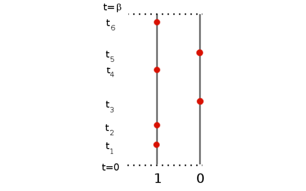
where in this case a path is specified by an bit string (call this the starting state) at time and a sequence of flips which occur in bits labeled at times (which are ordered), where each and for . Another way of specifying a path is to specify the path of each spin . So a path of the n spin system can be written . For each , specifies the th bit of the starting state as well as the times at which bit flips occur in bit j. Note that we only need to consider paths which flip each bit an even number of times, since only these paths occur with nonzero probability. An example of a path for a system with 2 spins is given in figure 20.
We now define in detail the Markov Chain which has limiting distribution It will be useful to define (for each ) to be the conditional probability distribution of the path of the th bit, conditioned on the remainder of the path being fixed.
As in [14], the update rule for the Monte Carlo algorithm consists of the following 3 steps:
- 1.
Randomly and uniformly choose a spin j (where ).
- 2.
Remove all flips in the path which occur in bit . Also remove the th bit from the starting state . This step corresponds to wholly removing the path of spin .
- 3.
Draw a new path (starting value and flip times) for spin j from the conditional distribution .
Of course, the nontrivial part of this algorithm is in specifying a procedure which executes step (3) in the above. To do this, the authors of reference [14] note that for any index , the diagonal part of the Hamiltonian can be written as
| (20) |
where and are operator valued functions of all except for . For a given path , we define for . The function ) is then piecewise constant, and for a given path can be written as
Although the above expression involves all the bit flips in the path, the function can actually only change value at times where bit flips occur in bits other than the th bit, since the operator does not involve . Let us then write
In this expression the times correspond to times at which bit flips occur in bits other than bit (also, ).
With this notation, the procedure of reference [14] that generates a new path for bit consists of the following:
- 1.
Compute the value of as a function of imaginary time along the path.
- 2.
In this step we generate boundary conditions for the path of bit at times . In other words we choose values such that at time the bit will be set to the value in the new path that we are generating. To do this, we sample the values for spin j at the times from their joint distribution, which is given by
where
and . We also define .
- 3.
Having chosen boundary conditions, we now generate subpaths for bit on each interval of length . Such a subpath is specified by a number of flips and the time offsets at which flips occur (note that the starting value of the bit is determined by the boundary conditions). The number of flips is restricted to be either even or odd depending on the boundary conditions that were chosen for this interval in the previous step. In this step, the subpath for each interval is drawn from the distribution
(21) - 4.
Put all the subpaths together to form a new path for bit on .
In section .1 we review the method outlined in [14] for sampling from the distribution in step (2) of the above. In section .2 we outline our method for sampling from the distribution , which differs from the method suggested in reference [14].
.1 Generating Boundary Conditions for A Single Spin Path
The prescription outlined in [14] for generating a set from the distribution
is as follows. First generate according to the distribution
(computing these probabilities involves multiplying two by two matrices). Then generate according to
Then generate from the distribution
and so on. Note that this generates the correct distribution since
.2 Algorithm for Sampling from the Single Spin Path Integral with Fixed Boundary Conditions
We now present an algorithm which samples from the normalized probability distribution over single spin paths for ( takes values in ). Here we only present the case of paths with boundary conditions and . The other three cases are completely analogous. We can parameterize such a path with fixed boundary conditions by the times at which changes value. Note that the number of such flips is odd due to our choice of boundary conditions. The distribution over paths that we aim to sample from is given by
| (22) |
It will also be useful for us to make the change of variables from the times to the waiting times defined by
Then the weight assigned to each path is
which we can also write as
The algorithm is as follows:
- 1.
Start at t=0 in state defined by the boundary conditions. Define Set i=1.
- 2.
Draw the waiting time until the next flip from the distribution
If then go to step 3. Otherwise define and set and repeat step 2.
- 3.
Take the path you have generated (which will in general be longer than ), and look at the segment . If this path satisfies the boundary condition at then take this to be the generated path. Otherwise, throw away the path and repeat from step (1).
We now show that this algorithm generates paths from the distribution (22). Before conditioning on the boundary conditions being satisfied, the probability of generating a sequence of waiting times in followed by any waiting time such that is given by
In the last line we have used the difference of squares formula to simplify consecutive terms: . When we condition on fixed boundary conditions (whatever they may be), this generates the correct distribution over paths. *