On the Newtonian limit of emergent NC gravity
and long-distance corrections

UWTHPh-2009-07

Harold Steinacker¹

Department of Physics, University of Vienna
Boltzmanngasse 5, A-1090 Wien, Austria

¹¹footnotetext: harold.steinacker@univie.ac.at

Abstract

We show how Newtonian gravity emerges on 4-dimensional non-commutative spacetime branes in Yang-Mills matrix models. Large matter clusters such as galaxies are embedded in large-scale harmonic deformations of the space-time brane, which screen gravity for long distances. On shorter scales, the local matter distribution reproduces Newtonian gravity via local deformations of the brane and its metric. The harmonic “gravity bag” acts as a halo with effective positive energy density. This leads in particular to a significant enhancement of the orbital velocities around galaxies at large distances compared with the Newtonian case, before dropping to zero as the geometry merges with a Milne-like cosmology. Besides these “harmonic” solutions, there is another class of solutions which is more similar to Einstein gravity. Thus the IKKT model provides an accessible candidate for a quantum theory of gravity.

1 Introduction

The aim of this paper is to study the physical properties of the effective (“emergent”) gravity which arises in matrix models such as the IKKT model, with emphasis on long-distance and cosmological aspects.

The presently accepted description for cosmology, known as $\Lambda$ CDM model, is able to reproduce the basic observational data. Its is based on the assumption that gravity is described by general relativity (GR), leading to the Friedmann equations which describe a homogeneous and isotropic universe. However, this requires a very delicate fine-tuning of the basic parameters in order to reproduce the observational constraints. The most problematic aspect is dark energy or the cosmological constant $\Lambda$ , which must be fine-tuned to $\Lambda\approx 2\times 10^{-3}eV$ on order to produce the apparent cosmic acceleration inferred from the type Ia supernovae data. The standard model also requires significant amounts of dark matter in order to reconcile the galactic rotation curves with GR: The rotation velocities of stars near or outside the visible bulk of typical galaxies does not decrease with radius as implied by GR resp. Newtonian gravity, rather it is more-or-less flat or even increasing. This is usually explained by postulating large dark matter halos around the galaxies, which however has never been observed directly.

These and other problems provide sufficient motivation to look for alternative descriptions of gravity, in particular at large distances. Indeed in spite of its undisputed success, general relativity has never been tested directly on cosmological scales. Finally, all attempts to define a quantum version of GR are faced with serious conceptual and technical difficulties.

In this paper, we show that matrix models, notably the IKKT matrix model [1], provide a very interesting alternative theory of gravity which might allow to resolve these problems. The geometric mechanism for gravity in these Yang-Mills matrix models was clarified recently [2, 3, 4], realizing related ideas [5, 6, 7, 8] in a concise framework. Space-time is described in terms of a 3+1-dimensional noncommutative (NC) brane solution embedded in ${\mathbb{R}}^{10}$ , i.e. a quantized space ${\cal M}_{\theta}\subset{\mathbb{R}}^{10}$ which carries a non-degenerate Poisson tensor $\theta^{\mu\nu}(x)$ . All matter and gauge fields live on this space-time brane, and there are no physical fields propagating in the ambient 10-dimensional space¹¹ 1 unlike in other braneworld scenarios such as [9, 10]. An effective dynamical metric $G^{\mu\nu}(x)$ arises on this space-time brane, which governs the kinetic term of all fields more-or-less as in GR. This metric is composed of the embedding metric $g_{\mu\nu}$ and the Poisson tensor, $G^{\mu\nu}\sim\theta^{\mu\mu^{\prime}}\theta^{\nu\nu^{\prime}}g_{\mu^{\prime}\nu^{\prime}}$ , and defines the effective gravity seen by matter and fields as in GR. However, the dynamics of the effective metric is not described by the Einstein equations.

An essential difference to general relativity is that the metric is not a fundamental degree of freedom, but arises effectively in terms of scalar fields describing the embedding of space-time ${\cal M}_{\theta}\subset{\mathbb{R}}^{10}$ , and the Poisson tensor $\theta^{\mu\nu}$ describing noncommutativity. This makes the dynamics of emergent NC gravity somewhat difficult to disentangle. In this paper, we obtain approximate solutions which correspond to static and somewhat localized matter distributions, having in mind galaxies and their stars inside. The bottom line is that large matter clusters such as galaxies are embedded in “gravity bags” or halos, which are deformations of the embedding ${\cal M}_{\theta}\subset{\mathbb{R}}^{10}$ with very long (galactic or cosmological) wavelength. These gravity bags turn out to screen gravity at large distances, and enclose an effective positive “vacuum energy”. Localized matter distributions such as stars then induce local deformation of this large-scale embedding, which leads to Newtonian gravity within these gravity bags at shorter scales.

The effective vacuum energy inside the gravity bags can be considerably larger than the currently preferred value in the $\Lambda$ CDM model, which – along with other contributions – leads to a significant enhancement of the (galactic) rotation velocities at large distances. This might provide an explanation of the observed galactic rotation curves without invoking large amounts of dark matter. Moreover, the effective Newton constant is determined by the large-scale deformation resp. the gravitational background, and therefore can vary somewhat in different locations of the universe.

The screening of gravity and the different physics of vacuum energy naturally leads to a consistent cosmological picture, where the localized matter distributions are embedded in a Milne-like cosmology [11]. This is in remarkably good agreement with basic observations, requiring considerably less fine-tuning than in the standard model. We briefly recall this cosmological solution in section 4.4, and show how the present results naturally fit into this cosmological context.

Due to the nonlinear nature of the problem, the results of this paper are somewhat incomplete and preliminary. However, the basic results concerning the Newtonian limit and the long-distance deviations from Newtonian gravity and GR are expected to be reliable. At short distances the approximations are less reliable, and a more complete analysis is required before seriously addressing e.g. the solar system precision tests. But in any case, it is remarkable how naturally emergent NC gravity seems to reproduce most of the basic observations, with far less fine-tuning than in the $\Lambda$ CDM model. Given the rigidity of the model and its perspective to define a full quantum theory of fundamental interactions, it certainly deserves to be studied very thoroughly.

2 The Matrix Model

We consider the following type of Yang-Mills matrix models

S_{YM}=-\Lambda_{0}^{4}\,{\rm Tr}\left(\frac{1}{4}[X^{a},X^{b}][X^{a^{\prime}},X^{b^{\prime}}]\eta_{aa^{\prime}}\eta_{bb^{\prime}}\,\,+\,\,\frac{1}{2}\,\overline{\Psi}\Gamma_{a}[X^{a},\Psi]\right)

(1)

where $\eta_{aa^{\prime}}=\mbox{diag}(-1,1,...,1)$ ; the Euclidean version of the model is obtained by replacing $\eta_{aa^{\prime}}$ with $\delta_{aa^{\prime}}$ . The degrees of freedom of this model are hermitian²² 2 in the Minkowski case, we will assume that the time-like matrices are anti-hermitian, see below. This is consistent with a real metric and action, and will be addressed in more detail elsewhere. matrices $X^{a}\,\in Mat(\infty,{\mathbb{C}})$ for $a=0,1,2,...,D-1$ , as well as Grassmann-valued matrices $\Psi$ which are spinors of $SO(D-1,1)$ resp. $SO(D)$ . The $\Gamma_{a}$ generate the Clifford algebra in $D$ dimensions. We introduced also an energy scale $\Lambda_{0}$ which gives the matrices $X^{a}$ the dimension of length. The action is invariant under the fundamental gauge symmetry

X^{\mu}\to U^{-1}X^{\mu}U,\quad\Psi\to U^{-1}\Psi U\qquad U\in{\cal U}({\cal H})

(2)

as well as a global $ISO(D-1,1)$ resp. $ISO(D)$ symmetry, where translations act as $X^{a}\to X^{a}+c^{a}\mbox{1 \kern-5.89996pt{\rm l}}$ . However there is no space-time or geometry to start with; space and geometry “emerge” only as solutions or backgrounds of the model. The models can be obtained as dimensional reduction of large- $N$ super-Yang-Mills theory to dimension zero. The IKKT model with $D=10$ is singled out by an extended matrix supersymmetry [1].

It is easy to see how space(time) arises in such a model³³ 3 This basic observation has been made by many authors including [12, 15, 13, 14], and it is obvious from the point of view of NC gauge theory [18, 16, 17].. Dropping the fermionic terms for now, the equations of motion

[X^{a},[X^{b},X^{a^{\prime}}]]\eta_{aa^{\prime}}=0

(3)

admit in particular $4$ -dimensional noncommutative or quantum spaces ${\cal M}_{\theta}\subset{\mathbb{R}}^{{10}}$ as solution. This means that we can split the set of matrices as

X^{a}=(X^{\mu},\phi^{i}),\qquad\mu=0,...,3,\,\,\,i=4,...,9

(4)

where the 4 generators $X^{\mu}$ are assumed to generate the full matrix algebra $Mat(\infty,{\mathbb{C}})$ , which is interpreted as space of (noncommutative) functions on ${\cal M}$ , i.e. $Mat(\infty,{\mathbb{C}})\cong{\cal C}_{\theta}({\cal M})$ . This is the basic idea of noncommutative geometry. The “scalar fields” $\phi^{i}=\phi^{i}(X^{\mu})$ are then functions of $X^{\mu}$ . The prototype of such a solution is the Moyal-Weyl quantum plane where $[X^{\mu},X^{\nu}]=i\overline{\theta}^{\mu\nu}\mbox{1 \kern-5.89996pt{\rm l}},\,\,\phi^{i}=0$ , but we will focus on the case of nontrivial $\phi^{i}$ here.

The basic hypothesis in is that space-time is described by such a quantum space solution of (3). We focus on the semi-classical limit of such quantum spaces, indicated by $\sim$ . Then the $\phi^{i}(x)$ define the embedding of a 4-dimensional submanifold⁴⁴ 4 cf. [19] for a different approach to NC submanifolds. ${\cal M}\subset{\mathbb{R}}^{10}$ , and

[X^{\mu},X^{\nu}]\sim i\theta^{\mu\nu}(x),\quad\mu,\nu=1,...,4

(5)

can be interpreted as Poisson structure on ${\cal M}$ . In particular, the matrices $X^{\mu}\sim x^{\mu}$ are interpreted as quantization of coordinate functions on ${\cal M}$ . Thus the matrix model provides preferred coordinates $x^{\mu}$ , which however have no physical meaning whatsoever. From the point of view of GR, they essentially “fix the gauge”, disposing of diffeomorphism invariance which does not make sense in the matrix model. Since gauge-dependent objects are always unphysical, this has no implications on the physical content of the model.

All physical fields in this model arise from fluctuations in the matrix model around such a background (leading to nonabelian⁵⁵ 5 In the nonabelian case the background solution is generalized to include a $\mathfrak{s}\mathfrak{u}(n)$ factor, see e.g. [4, 20] gauge fields and scalars) and from the fermionic matrices $\Psi$ . Since $Mat(\infty,{\mathbb{C}})\cong{\cal C}_{\theta}({\cal M})$ by assumption, it follows that they all live only on the brane ${\cal M}$ , and there is no physical higher-dimensional “bulk” which could carry any propagating degrees of freedom. This does not exclude the existence of compactified physical extra dimensions in the matrix model, but these are different backgrounds which we will leave aside for simplicity here.

Emergent geometry.

The Poisson tensor $\theta^{\mu\nu}(x)$ not only governs the noncommutative structure of ${\cal M}$ , it also plays a crucial but implicit role in the low-energy effective action and the metric on ${\cal M}$ . We need to assume that it is non-degenerate, so that its inverse

\theta^{-1}_{\mu\nu}(x)\,

(6)

defines a symplectic 2-form on ${\cal M}$ . Then the trace on $Mat(\infty,{\mathbb{C}})$ is given semi-classically by the volume of this symplectic form,

	$\displaystyle(2\pi)^{2}\,Trf$	$\displaystyle\sim$	$\displaystyle\int d^{4}x\,\rho(x)\,f$
	$\displaystyle\rho(x)$	$\displaystyle=$	$\displaystyle(\det\theta^{-1}_{\mu\nu})^{1/2}.$		(7)

We can now extract the semi-classical limit of the matrix model and its physical meaning. To understand the effective geometry of ${\cal M}^{4}$ , consider a test-particle on ${\cal M}^{4}$ , modeled by a scalar field $\varphi$ for simplicity (this could be e.g. an $su(k)$ component of $\phi^{i}$ ). In order to preserve gauge invariance, the kinetic term must have the form

\displaystyle S[\varphi]

\displaystyle\equiv

\displaystyle-Tr[X^{a},\varphi][X^{b},\varphi]\eta_{ab}=-Tr\left([X^{\mu},\varphi][X^{\nu},\varphi]\eta_{\mu\nu}+[\phi^{i},\varphi][\phi^{j},\varphi]\delta_{ij}\right).

(8)

Expressing the $\phi^{i}$ in terms of $X^{\mu}$ and using

[\phi^{i},f(X^{\mu})]\,\sim\,i\theta^{\mu\nu}\partial_{\mu}\phi^{i}\partial_{\nu}f

(9)

this kinetic term can be cast into covariant form

\displaystyle S[\varphi]

\displaystyle\sim

\displaystyle\frac{1}{(2\pi)^{2}}\,\int d^{4}x\;|G_{\mu\nu}|^{1/2}\,G^{\mu\nu}(x)\partial_{\mu}\varphi\partial_{\nu}\varphi\,,

(10)

where [3]

$\displaystyle G^{\mu\nu}(x)$	$\displaystyle=$	$\displaystyle e^{-\sigma}\,\theta^{\mu\mu^{\prime}}(x)\theta^{\nu\nu^{\prime}}(x)g_{\mu^{\prime}\nu^{\prime}}(x)$	(11)
$\displaystyle e^{-\sigma}$	$\displaystyle=$	$\displaystyle\rho\,\|g_{\mu\nu}(x)\|^{-\frac{1}{2}},$
$\displaystyle g_{\mu\nu}(x)$	$\displaystyle=$	$\displaystyle\partial_{\mu}x^{a}\partial_{\mu}x^{a}\,\,=\eta_{\mu\nu}(x)+\partial_{\mu}\phi^{i}\partial_{\mu}\phi^{j}\delta_{ij}.$	(12)

Here $g_{\mu\nu}(x)$ is the metric induced on ${\cal M}^{4}\subset{\mathbb{R}}^{10}$ via pull-back of $\eta_{ab}$ . Therefore the kinetic term for $\varphi$ on ${\cal M}^{4}_{\theta}$ is governed by the metric $G_{\mu\nu}(x)$ , which depends on the Poisson tensor $\theta^{\mu\nu}$ and the embedding metric $g_{\mu\nu}(x)$ . It turns out that the same metric also governs nonabelian gauge fields [4] and fermions [3] in the matrix model, hence $G_{\mu\nu}$ must be interpreted as gravitational metric. There is no need and no room for invoking any “principles”.

We note that

|G_{\mu\nu}(x)|=|g_{\mu\nu}(x)|,

(13)

which means that the Poisson tensor $\theta^{\mu\nu}$ does not enter the Riemannian volume at all. This is important for stabilizing flat space, as we will see. Note also that the matrix model action (1) can be written in the semi-classical limit as

S_{YM}=-\Lambda_{0}^{4}\,Tr\frac{1}{4}[X^{a},X^{b}][X^{a^{\prime}},X^{b^{\prime}}]\eta_{aa^{\prime}}\eta_{bb^{\prime}}\,\sim\,\frac{1}{(2\pi)^{2}}\,\int d^{4}x\,\Lambda_{0}^{4}\,\rho(x)\eta(x),

(14)

where

\displaystyle\eta(x)

\displaystyle=

\displaystyle\frac{1}{4}e^{\sigma}\,G^{\mu\nu}(x)g_{\mu\nu}(x).

(15)

Covariant equations of motion.

As shown in [3], the basic matrix equations of motion (3) can now be cast into a covariant form as follows:

$\displaystyle\square_{G}\phi^{i}$	$\displaystyle=$	$\displaystyle 0$	(16)
$\displaystyle\square_{G}x^{\mu}$	$\displaystyle=$	$\displaystyle 0$	(17)
$\displaystyle\nabla_{G}^{\eta}(e^{\sigma}\theta^{-1}_{\eta\nu})\,$	$\displaystyle=$	$\displaystyle\,e^{-\sigma}\,G_{\mu\nu}\,\theta^{\mu\gamma}\,\partial_{\gamma}\eta(x)$	(18)

where we consider $x^{\mu}\sim X^{\mu}$ as a scalar function on ${\cal M}$ , consistent with the ambiguity of the splitting $X^{a}=(X^{\mu},\phi^{i})$ into coordinates and scalar fields. Here $\nabla_{G}$ denotes the Levi-Civita connection with respect to the effective metric $G^{\mu\nu}$ . In particular, such on-shell geometries imply [3]

\Gamma^{\mu}=0

(19)

for the preferred matrix coordinates $x^{\mu}$ , which in general relativity would be interpreted as gauge condition. Furthermore, it turns out that (18) is in fact a consequence of a matrix Noether theorem due to the translational symmetry $X^{a}\to X^{a}+c^{a}\mbox{1 \kern-5.89996pt{\rm l}}$ , and is therefore protected from quantum corrections [4]. It provides the relation between the noncommutativity $\theta^{\mu\nu}(x)$ and the metric $G^{\mu\nu}$ . Since (18) has essentially the form of covariant Maxwell equations coupled to an external current, it should have a unique solution for a given “boundary condition”

\theta_{\mu\nu}(x)\,\to\,\bar{\theta}_{\mu\nu}=const\qquad\mbox{for}\quad|x|\to\infty

(20)

up to radiational contributions, which play the role of gravitational waves here [5, 2].

Relation with string theory.

The IKKT matrix model was proposed originally as a non-perturbative definition of IIB string theory on ${\mathbb{R}}^{10}$ . From this point of view, ${\cal M}_{\theta}$ could be interpreted as a brane with open string metric $G^{\mu\nu}$ , while $g_{\mu\nu}$ could be viewed as closed string metric in the 10D bulk. Indeed there are also other solutions of the matrix model, in particular 10D solutions. Notably graviton scattering has been studied in this and related matrix models; for an incomplete list of references see e.g. [23, 12, 1, 15, 24, 14, 13, 22, 25] and references therein. Most of this work was based on a different kind of block-matrix backgrounds, and to simple geometries in the NC case. The essential point here is to consider general 4-dimensional NC brane solutions, without physical 10D bulk. On such a background, the matrix model can be viewed as NC gauge theory [16, 17], which includes gravity as we have seen. In this way the strength of string theory (notably the good behavior under quantization) is preserved while the main problems (lack of predictivity) are avoided. In particular, the matrix model should be viewed as background-independent here, since there is no physical space-time to start with.

A natural question arises how the present results relate to the BFSS matrix model [23] of (M)atrix theory, which involves 9 matrices depending on a classical “time” parameter. This model is not unrelated to the IKKT model as pointed out in [1], and some version of the present mechanism should be realized there as well; this should be studied elsewhere. We only want to stress here that the space-time brane ${\cal M}$ must be entirely noncommutative in the present framework, i.e. $\theta^{\mu\nu}$ must be non-degenerate. Nevertheless a conventional physical picture emerges at scales larger than $\Lambda_{NC}$ , and there is no need for a classical time parameter. Hence the IKKT model is more natural for the mechanism of emergent gravity. It is also very interesting that some evidence for 4-dimensional space-time (rather than some other dimension) emerging in that model has been found [26].

The topic of membranes and matrix models has of course a long history, cf. also [28, 29, 27]. It is also interesting to compare the present approach with other models of emergent gravity, see e.g. [30] and references therein.

2.1 Self-dual solutions and $g_{\mu\nu}=G_{\mu\nu}$

A simple class of solutions of (18) is given by “self-dual” 2-forms $\theta^{-1}_{\mu\nu}(x)$ which satisfy

\nabla^{\mu}\theta^{-1}_{\mu\nu}=0,\qquad g_{\mu\nu}=G_{\mu\nu}.

(21)

To see this, consider (at a point $x$ ) a local coordinate system where $g_{\mu\nu}=\mbox{diag}(s,1,1,1)$ (with $s=\pm 1$ in the Euclidean resp. Minkowski case) and $\theta^{\mu\nu}$ has the form

\sqrt{\rho}\,\theta^{\mu\nu}=\left(\begin{array}[]{cccc}0&0&0&-\sqrt{s}\alpha\\ 0&0&\pm\alpha^{-1}&0\\ 0&\mp\alpha^{-1}&0&0\\ \sqrt{s}\alpha&0&0&0\end{array}\right)\,;

(22)

this can always be achieved using a $SO(4)$ resp. $SO(1,3)$ transformation⁶⁶ 6 Note that we assume that $\theta^{0i}$ is imaginary in the Minkowski case. This might appear strange, but it is natural having in mind a Wick rotation $x^{0}=it$ , and it is essential for $g_{\mu\nu}=G_{\mu\nu}$ . This should be addressed in more detail elsewhere. at the point $x$ . Clearly this is (anti-) self-dual $\star\theta^{-1}=\pm\sqrt{s}\,\theta^{-1}$ if and only if $\alpha^{2}=1$ , where $\star$ denotes the Hodge star and $\theta^{-1}=\theta^{-1}_{\mu\nu}dx^{\mu}\wedge dx^{\nu}$ . On the other hand,

G^{\mu\nu}=\rho\theta^{\mu\mu^{\prime}}\theta^{\nu\nu^{\prime}}g_{\mu^{\prime}\nu^{\prime}}=\mbox{diag}(s\alpha^{2},\alpha^{-2},\alpha^{-2},\alpha^{2})

(23)

at the point $x$ , hence $e^{-\sigma}\eta=\frac{1}{2}(\alpha^{2}+\alpha^{-2})$ . Therefore $\star\theta^{-1}=\pm\sqrt{s}\,\theta^{-1}$ if and only if $g_{\mu\nu}=G_{\mu\nu}$ , or equivalently $e^{\sigma}=\eta$ . It is then easy to see that in this self-dual case (18) reduces to $\nabla^{\mu}\theta^{-1}_{\mu\nu}=0$ , which holds identically since $d\star\theta^{-1}=d\theta^{-1}=0$ .

Such (anti-)self-dual closed 2-forms $\theta^{-1}$ with constant asymptotics $\theta^{-1}_{\mu\nu}(x)\to\overline{\theta}^{-1}_{\mu\nu}$ as $x\to\infty$ always exist, at least on asymptotically flat spaces. This can be understood by interpreting $\theta^{-1}$ as sourceless electromagnetic field with constant field strength at infinity. Indeed, we only have to solve $d\star F=0,\,\,F=dA$ with suitable asymptotics $F\to\overline{F}$ as $r\to\infty$ , and define $\theta^{-1}$ to be the (anti-)selfdual component of $F$ .

In this self-dual case $g_{\mu\nu}=G_{\mu\nu}$ , the bare matrix model action (14) becomes

S_{MM}=\Lambda_{0}^{4}\int d^{4}x\,\rho\eta=\Lambda_{0}^{4}\int d^{4}x\,\rho e^{\sigma}=\int d^{4}x\,\sqrt{|G_{\mu\nu}|}\Lambda_{0}^{4}=\int d^{4}x\,\sqrt{|g_{\mu\nu}|}\Lambda_{0}^{4}

(24)

which is precisely the form of the vacuum energy resp. brane tension, interpreted as cosmological constant in GR. We collect all such (bare and induced) terms in

S_{vac}=-2\int d^{4}x\,\sqrt{|g_{\mu\nu}|}\Lambda_{1}^{4}

(25)

denoting with $\Lambda_{1}^{4}$ the sum of $\Lambda_{0}^{4}$ and the induced quantum-mechanical vacuum energy; the above sign is essential for stability reasons, cf. section 4.3. We also recall that the effective Yang-Mills coupling constant for the basic $SU(n)$ gauge fields on ${\cal M}^{4}$ is given by [4]

g^{2}_{YM}=\Lambda_{0}^{-4}\,e^{-\sigma}\sim\Lambda_{0}^{-4}\,\Lambda_{NC}^{4},

(26)

so that $g_{YM}=O(1)$ amounts to

\Lambda_{0}\sim\Lambda_{NC}.

(27)

Let us briefly discuss deviations from the self-dual case $g_{\mu\nu}\neq G_{\mu\nu}$ . These arise from (abelian) variations $\delta x^{\mu}=\theta^{\mu\nu}A_{\nu}$ of the tangential matrix degrees of freedom resp. “would-be $U(1)$ gauge fields”, which lead to $\delta\theta^{-1}_{\mu\nu}=F_{\mu\nu}$ where $F_{\mu\nu}$ is the corresponding field strength. The corresponding propagating degrees of freedom behave as gravitational waves, with metric fluctuations $h_{\mu\nu}=G_{\nu\nu^{\prime}}\theta^{\nu^{\prime}\rho}F_{\rho\mu}+G_{\mu\mu^{\prime}}\theta^{\mu^{\prime}\rho}F_{\rho\nu}\,+\frac{1}{2}G_{\mu\nu}F_{\rho\eta}\theta^{\rho\eta}$ [5, 2]. In the presence of matter, we expect additional source terms on the rhs of equations (16) – (18). While matter is not charged under this gravitational $U(1)$ , it is expected to induce e.g. dipole (and higher multipole) excitations of $F_{\mu\nu}$ . This would lead to short-distance modifications of the metric which decay more rapidly than $\frac{1}{r}$ . We therefore simply ignore such effects here, and consider only the simplest “self-dual” solutions with $g_{\mu\nu}=G_{\mu\nu}$ .

2.2 Static metric deformations

We focus on deformations of the embedding ${\cal M}^{4}\subset{\mathbb{R}}^{D}$ through the scalar fields $\phi^{i}$ with embedding metric (12)

	$\displaystyle g_{\mu\nu}$	$\displaystyle=$	$\displaystyle\eta_{\mu\nu}+\partial_{\mu}\phi^{i}\partial_{\nu}\phi^{i}$		(28)
		$\displaystyle\equiv$	$\displaystyle\eta_{\mu\nu}+h_{\mu\nu},$		(28)

and assume that $G_{\mu\nu}=g_{\mu\nu}$ , i.e. that $\theta^{\mu\nu}$ is self-dual w.r.t. $g_{\mu\nu}$ as discussed above. This is an ansatz⁷⁷ 7 In fact one of the main difficulties in this context is to understand and disentangle the effects of the embedding $\phi^{i}$ versus the NC structure $\theta^{\mu\nu}$ . We hope that this paper helps to clarify this issue. In particular, the ansatz in [2] with trivial embedding but nontrivial $\theta^{\mu\nu}$ may not be realized in the presence of matter. which may not be completely appropriate, but it is expected to give the correct long-distance physics in the static case since corrections due to $G_{\mu\nu}\neq g_{\mu\nu}$ lead to be short-distance effects and gravitational waves.

We furthermore focus on static metrics $g_{\mu\nu}$ , corresponding to static and somewhat localized matter distributions. One goal is to obtain the analog of the Schwarzschild solution at least in some regime. Since $h_{\mu\nu}$ is quadratic in $\phi$ , we cannot restrict ourselves to linearized fluctuations in $\phi$ around flat Minkowski space. We must include at least quadratic terms in $\phi$ , which makes the analysis somewhat non-trivial. Nevertheless we will find a class of solutions which appear to give the appropriate description of objects such as galaxies sparsely embedded in flat Minkowski space. This also fits naturally in the context of the cosmological solutions [11], as discussed in section 4.4.

Some insight can be gained by observing that the metric fluctuation $h_{\mu\nu}$ is closely related to the energy-momentum tensor of the massless scalar fields $\phi^{i}$ ,

	$\displaystyle T_{\mu\nu}^{\phi}$	$\displaystyle=$	$\displaystyle\partial_{\mu}\phi\partial_{\nu}\phi-\frac{1}{2}\eta_{\mu\nu}(\eta^{\alpha\beta}\partial_{\alpha}\phi\partial_{\beta}\phi)=h_{\mu\nu}-\frac{1}{2}\eta_{\mu\nu}\,h,$
	$\displaystyle h$	$\displaystyle=$	$\displaystyle\eta^{\alpha\beta}h_{\alpha\beta}=-\eta^{\mu\nu}T_{\mu\nu}^{\phi}.$		(29)

In particular, the effective Newtonian potential is related to the energy density of a free scalar field,

2U(x)=-h_{00}=-T_{00}^{\phi}+\frac{1}{2}\,h\approx-\frac{1}{2}T_{00}^{\phi}

(30)

assuming $T_{ij}^{\phi}\approx 0$ in the last step. Hence a static metric fluctuation corresponds to a a scalar field excitation with static energy-momentum tensor. Furthermore, since $\phi$ in vacuum satisfies the free wave equation (16), it will decay like $\frac{1}{r}$ outside of matter distributions, suggesting a $U(r)\sim\frac{1}{r^{2}}$ behavior for the gravitational potential. This appears very bad at first, since this is not the usual $U(r)\sim\frac{1}{r}$ law of Newtonian gravity.

The resolution of this puzzle is as follows: the relevant non-singular harmonic excitations necessarily have some finite wavelength, $\phi^{i}\sim\frac{\sin(\omega r)}{\omega r}e^{i\omega t}$ . These are localized excitations resp. “gravity bags”, which we will argue to have very long (astronomical) wavelength $\omega$ . This leads to a long-distance screening of gravity with $U(r)\sim\frac{1}{r^{2}}$ . However the crucial point is that inside these gravity bags (in particular inside of galaxies, say), the local matter distribution does indeed lead to the standard $U(r)\sim\frac{1}{r}$ , as we will show. Newtonian gravity therefore arises as a “short-distance” effect on the harmonically embedded spacetime brane.

Basic “rotating” embedding.

We consider brane embedding ${\cal M}^{4}\subset{\mathbb{R}}^{D}$ which are small deformations of flat Minkowski space, with the following structure:

\displaystyle x^{A}=\left(\begin{array}[]{c}x^{0}\\ x^{i}\\ \phi^{i}\end{array}\right)=\left(\begin{array}[]{c}t\\ x^{i}\\ g(x)\,\left(\begin{array}[]{c}\cos(\omega t)\\ \sin(\omega t)\end{array}\right)\\ \end{array}\right)

where $g(x)$ is independent of $t$ and $g(x)\to 0$ as $r\to\infty$ . There might be additional components in this ansatz. We stress that the $\phi^{i}$ comprise two space-like components which rotate with $t$ , rather than just of its components⁸⁸ 8 The time-like component(s) could have similar nontrivial embeddings. This should be elaborated elsewhere.. We will see in section 4.4 that due to its flat asymptotics, this type of embedding fits naturally into the context of the cosmological solutions obtained in [11]. An important feature of this ansatz is

\partial_{0}\phi^{k}\partial_{i}\phi^{k}=0,

(40)

leading to a static metric

ds^{2}=-(1-\omega^{2}\,g^{2})\,dt^{2}+(\delta_{ij}+\partial_{i}g\partial_{j}g)dx^{i}dx^{j}

(41)

This is consistent with the fact that there is no energy flux associated to standing waves. There might be several components of $g\to g^{i}$ whose contributions will simply add up; this will not alter the essential conclusions below. Clearly the rotating embedding with $\omega\neq 0$ must be responsible for Newtonian gravity, which cannot be reproduced with a purely static embedding. Additional components might be necessary to comply e.g. with the detailed solar system constraints. The embedding functions $\phi^{i}$ must be determined by solving the equations of motion in the presence of matter, which will be done below. Note that the preferred “matrix coordinates” $x^{\mu}$ automatically satisfy the e.o.m. $\square_{g}x^{\mu}=0$ in vacuum (16), (17); therefore we will only consider the equations of motion for $\phi^{i}$ below.

3 Coupling to matter and effective gravity

3.1 Effective action and equations of motion with matter

In this section we derive the equations of motion for gravity coupled to matter in the semi-classical limit, assuming $g_{\mu\nu}=G_{\mu\nu}$ as discussed above. Our starting point is the semi-classical effective action of the matrix model (25) together with the action for matter, and the Einstein-Hilbert action $R[G]=R[g]$ which is induced at one-loop⁹⁹ 9 Assuming a cutoff $\Lambda_{4}$ , which is the cutoff for $N=4$ SUSY in the IKKT model, see [32, 31]

S=\int d^{4}x\sqrt{|g|}\,(\Lambda_{4}^{2}R-2\Lambda_{1}^{4})+S_{\rm matter}.

(42)

Now recall

$\displaystyle\delta\int\sqrt{\|g\|}$	$\displaystyle=$	$\displaystyle\delta\sqrt{-\det g}=\frac{1}{2}\sqrt{\|g\|}\,g^{\mu\nu}\delta g_{\mu\nu},$
$\displaystyle\delta\int\sqrt{\|g\|}\,R$	$\displaystyle=$	$\displaystyle-\sqrt{\|g\|}\,{\cal G}^{\mu\nu}\delta g_{\mu\nu}$
$\displaystyle\delta S_{\rm matter}$	$\displaystyle=$	$\displaystyle 8\pi\sqrt{\|g\|}\,T^{\mu\nu}\delta g_{\mu\nu}$	(43)

where ${\cal G}^{\mu\nu}=R^{\mu\nu}-\frac{1}{2}g^{\mu\nu}R$ is the Einstein tensor, and $T^{\mu\nu}$ is the energy-momentum tensor for matter (recall that matter and fields couple to the effective metric essentially in the standard way). The crucial point is now that the fundamental geometrical degrees of freedom are not the $g_{\mu\nu}$ , but the embedding fields $\phi^{i}$ as well as $X^{\mu}$ resp. $\theta^{\mu\nu}$ . In the self-dual case $g_{\mu\nu}=G_{\mu\nu}$ , the most general variation can thus be decomposed into variations of $g_{\mu\nu}=\eta_{\mu\nu}+\partial_{\mu}\phi^{i}\partial_{\nu}\phi^{i}=G_{\mu\nu}$ and variations of $\theta^{\mu\nu}$ . The e.o.m. for $\theta^{\mu\nu}$ are satisfied¹⁰¹⁰ 10 This however amounts to neglecting matter contributions to $\theta^{\mu\nu}$ , as discussed before. For geometries with non-selfdual $\theta^{\mu\nu}$ this derivation must be refined. due to (21). The variation of $S$ with respect to the fundamental fields $\phi^{i}$ can be written using $\delta g_{\mu\nu}=\partial_{\mu}\phi^{i}\partial_{\nu}\delta\phi^{i}+\partial_{\mu}\delta\phi^{i}\partial_{\nu}\phi^{i}$ as

\delta S=\int d^{4}x\sqrt{|g|}\,\delta g_{\mu\nu}{\cal H}^{\mu\nu}=-2\int\delta\phi^{i}\partial_{\mu}(\sqrt{|g|}\,{\cal H}^{\mu\nu})\partial_{\nu}\phi^{i}

(44)

up to boundary terms, where

{\cal H}^{\mu\nu}=8\pi T^{\mu\nu}-\Lambda_{4}^{2}{\cal G}^{\mu\nu}-\Lambda_{1}^{4}g^{\mu\nu}.

(45)

This leads to the equations of motion for $\phi^{i}$

\displaystyle\partial_{\mu}(\sqrt{|g|}\,{\cal H}^{\mu\nu}\partial_{\nu}\phi)=0,

(46)

which using the identity $\nabla_{\mu}V^{\mu}\equiv\frac{1}{\sqrt{g}}\partial_{\mu}(\sqrt{g}\,V^{\mu})$ can be written as

\displaystyle\Lambda_{1}^{4}\square_{g}\phi

\displaystyle=

\displaystyle(8\pi T^{\mu\nu}-\Lambda_{4}^{2}{\cal G}^{\mu\nu})\nabla_{\mu}\partial_{\nu}\phi+8\pi(\nabla_{\mu}T^{\mu\nu})\partial_{\nu}\phi

(47)

recalling $\nabla_{\mu}{\cal G}^{\mu\nu}=0$ . This equation has 2 types (“branches”) of solutions:

1.

“Einstein branch”:

Clearly every solution of the Einstein equations

$\Lambda g^{\mu\nu}+{\cal G}^{\mu\nu}=8\pi G\,T^{\mu\nu}$ (48)

is also a solution of ${\cal H}^{\mu\nu}=0$ (47), upon identifying

$\frac{1}{G}=\Lambda_{4}^{2}\qquad\frac{\Lambda}{G}=\Lambda_{1}^{4}.$ (49)

Indeed using general embedding theorems [33], any solution of the E-H equations can be realized (locally) using embeddings in $D\geq 10$ . This should provide an interesting realization of Einstein gravity within matrix models, with technical advantages over other approaches in particular for quantization. Recall however that we assumed $G_{\mu\nu}=g_{\mu\nu}$ , which will not always hold; thus there will be some modifications of the Einstein equations due to $\theta^{\mu\nu}(x)$ . On the other hand, this Einstein branch would presumably lead to the same problematic aspects of GR, notably fine-tuning issues in cosmology. In this paper we will focus on the second kind of solution, which leads to significant and very interesting deviations from GR at long distances.
2.

“Harmonic branch”:

Besides to the above solutions, there are additional solutions of (47) with

$\partial_{\mu}(\sqrt{|g|}\,{\cal H}^{\mu\nu}\partial_{\nu}\phi)=0,\qquad{\cal H}^{\mu\nu}\neq 0$ (50)

The prototype of such a solution without matter is flat Minkowski space $\phi^{i}=0$ with $\Lambda_{1}>0$ . More generally if the vacuum energy dominates the matter density, then (47) reduces to $\square_{g}\phi\approx 0$ , leading essentially to minimal surfaces which will be deformed in the presence of matter. This in turn leads to the near-realistic cosmological solutions of FRW type found in [11] with Milne-like late-time behavior, which are stable and largely insensitive to the detailed matter content. Another attractive feature of this harmonic branch is that its quantization should be comparably simple, as the embedding fields $\phi^{i}$ are governed in vacuum by a simple action with positive excitation spectrum, cf. section 4.3.

We will simply assume in the following that $\Lambda_{2}^{4}{\cal G}^{ij}$ can be neglected in the static case. This is however far from trivial, since the simple ansatz (2.2) will generally not lead to ${\cal G}^{ij}\approx 0$ . There are 2 ways how this might nevertheless be justified: either a more sophisticated ansatz taking into account $\theta^{\mu\nu}$ will imply ${\cal G}^{ij}\approx 0$ , or $\Lambda_{4}^{2}$ is much smaller than the Planck scale. The latter is in fact very appealing as we will see. In any case we focus on the harmonic branch in this paper, since it leads to very interesting long-distance modifications of Newtonian gravity which is the main topic of this paper.

3.2 Perturbations of flat Minkowski space-time

For simplicity we focus on perturbations of flat Minkowski space, and only consider the case of “weak” gravity, i.e.

g_{\mu\nu}=\eta_{\mu\nu}+h_{\mu\nu}

(51)

keeping only terms linear in $h_{\mu\nu}=\partial_{\mu}\phi^{i}\partial_{\nu}\phi^{i}$ . The e.o.m. (47) then simplifies to

\square_{\eta}\phi=\frac{8\pi}{\Lambda_{1}^{4}}\,\tilde{T}^{\mu\nu}\partial_{\mu}\partial_{\nu}\phi,\qquad\tilde{T}^{\mu\nu}\equiv T^{\mu\nu}-\frac{\Lambda_{4}^{2}}{8\pi}{\cal G}^{\mu\nu}

(52)

using¹¹¹¹ 11 The conservation law for $T^{\mu\nu}$ is not entirely evident in the matrix model, in particular for fermions which have a non-standard spin connection [34]. Nevertheless it is expected to hold at least to a very good approximation since the matter action almost coincides with the usual one. $\nabla_{\mu}T^{\mu\nu}=0$ . We also replace $\square_{g}\approx\square_{\eta}$ to leading approximation. In the case of a static mass distribution $\rho$ , we assume furthermore that

\tilde{T}_{00}=\rho(x)\equiv\rho^{matter}(x)-\rho^{curv}(x)\geq 0,\qquad\rho_{curv}=\frac{\Lambda_{4}^{2}}{8\pi}{\cal G}^{00}

(53)

and $\tilde{T}_{ij}\approx 0$ as discussed above¹²¹² 12 One might think that due to the Einstein equations, $\rho=\rho_{matter}-\rho_{grav}=0$ would drop out of the harmonic equation. This is not the case here, as the Einstein equations do not hold in this form.. Then (52) can be written using $\square=-\partial_{t}^{2}+\Delta$ as

\Delta\phi=(1+\frac{8\pi}{\Lambda_{1}^{4}}\rho(x))\partial_{0}^{2}\phi.

(54)

Note also that

	$\displaystyle\partial^{\mu}h_{\mu\nu}$	$\displaystyle=$	$\displaystyle(\partial_{\mu}\phi)(\partial^{\mu}\partial_{\nu}\phi)+(\square\phi)(\partial_{\nu}\phi)$		(55)
		$\displaystyle=$	$\displaystyle\frac{1}{2}\partial_{\nu}h+(\frac{8\pi}{\Lambda_{1}^{4}}\tilde{T}^{\alpha\beta}\partial_{\alpha}\partial_{\beta}\phi)(\partial_{\nu}\phi)$		(55)

so that $h_{\mu\nu}$ satisfies the “harmonic gauge” $\partial^{\mu}h_{\mu\nu}=\frac{1}{2}\partial_{\nu}h$ up to corrections due to matter and curvature.

3.2.1 Harmonic gravity bags

We are mainly interested in static spacetime-geometries in this paper. Thus consider the following localized excitation of the embedding (2.2)

\phi^{i}(x,t)=g(x)e^{i\omega t}=g(x)\left(\begin{array}[]{c}\cos(\omega t)\\ \sin(\omega t)\end{array}\right)

(56)

with some very small $\omega$ , leading to the static metric (41)

ds^{2}=-(1-\omega^{2}\,g^{2})\,dt^{2}+(\delta_{ij}+\partial_{i}g\partial_{j}g)dx^{i}dx^{j}.

(57)

For $\rho=0$ and neglecting the curvature corrections $\Lambda_{4}^{2}{\cal G}_{\mu\nu}$ , the equation of motion (54) becomes

\square\phi_{0}(x)=0,\qquad\Delta g_{0}(x)=-\omega^{2}g_{0}(x).

(58)

Consider first the case of a spherical wave, where this equation reduces to

\partial_{r}(r^{2}g^{\prime})+\omega^{2}r^{2}g(r)=0.

(59)

The unique spherically symmetric solution which is regular at the origin and decays as $r\to\infty$ is given by

	$\displaystyle g_{0}(r)$	$\displaystyle=$	$\displaystyle g_{0}\frac{\sin(\omega r)}{\omega r},$
	$\displaystyle\phi_{0}(x)$	$\displaystyle=$	$\displaystyle g_{0}(r)\,e^{i\omega t}\,=\,g_{0}(r)\,\left(\begin{array}[]{c}\cos(\omega t)\\ \sin(\omega t)\end{array}\right)$

with radial wavelength given by

L_{\omega}=\frac{\pi}{\omega}.

(63)

Near the origin, we can write

	$\displaystyle g_{0}(r)$	$\displaystyle=$	$\displaystyle g_{0}\frac{\sin(\omega r)}{\omega r}\approx g_{0}(1-\frac{1}{6}\omega^{2}r^{2}+...),$
	$\displaystyle g^{\prime}(r)$	$\displaystyle=$	$\displaystyle g_{0}\Big(\frac{\cos(\omega r)}{r}-\frac{\sin(\omega r)}{\omega r^{2}}\Big)\approx g_{0}(-\frac{1}{3}\omega^{2}r+\frac{1}{30}\omega^{4}r^{3}+O(r^{5})).$		(64)

Note that $g^{\prime}$ is regular at the origin, and decays like $\frac{1}{r}$ as $r\to\infty$ . The effective metric (41) is

ds^{2}=-(1-\omega^{2}\,g(r)^{2})\,dt^{2}+(1+(g^{\prime})^{2})dr^{2}+r^{2}d\Omega^{2},

(65)

which allows to read off the effective gravitational potential: a static test particle in this metric perturbation feels an effective gravitational potential

\displaystyle g_{00}=-(1+2U_{0}),\qquad 2U_{0}(r)

\displaystyle=

\displaystyle-\omega^{2}\,g(r)^{2}=-\omega^{2}g_{0}^{2}\Big(\frac{\sin(\omega r)}{\omega r}\Big)^{2},

(66)

which satisfies

	$\displaystyle U_{0}(r)$	$\displaystyle\sim$	$\displaystyle-\omega^{2}\frac{1}{r^{2}},\qquad r\to\infty$		(67)
	$\displaystyle\Delta U_{0}(r)$	$\displaystyle=$	$\displaystyle g_{0}^{2}\omega^{4},\qquad\quad r\sim 0$		(68)

The last equation will be interpreted later in terms of an effective gravitational constant/vacuum energy $\Lambda_{\rm eff}$ (82) inside the bag. For large distances, $U(r)$ leads to a rapidly decreasing attractive gravitational force with range $L_{\omega}$ . This might appear strange at first, since such vacuum excitations do not exist in general relativity. However, they are not expected to survive in this naked form: Due to their attractive gravitational force, matter will tend to accumulate inside, and these “gravity bags” will typically enclose matter with $\rho\neq 0$ . In particular, large clusters of matter such as galaxies will be embedded in such “gravity bags”. The essential point is that the matter within such a gravity bag will experience Newtonian gravity, as we will show next.

3.2.2 Spherically symmetric mass distribution and Newtonian limit

We now show how Newtonian gravity arises in the simplest case of spherically symmetric localized mass distributions, due to a local deformation of the above harmonic gravity bag. This will lead moreover to significant long-distance deviation from Newtonian gravity and GR. Basically, gravity is confined within the bag, which also contains an effective vacuum energy. The case of a more general mass distribution will be studied in section 4. This will clarify the significance of the gravity bag which we simply assume here.

Consider a spherically symmetric mass distribution around the origin within the radius $r_{M}$ . For $r>r_{M}$ , the corresponding solution of (54) with the “static” ansatz (56) must have the form

	$\displaystyle\phi^{i}$	$\displaystyle=$	$\displaystyle g(r)e^{i\omega t},$
	$\displaystyle g(r)$	$\displaystyle=$	$\displaystyle g_{0}\frac{\sin(\omega r+\delta)}{\omega r}\quad\sim\,\,g_{0}(\cos(\delta)+\frac{\sin(\delta)}{\omega r})$		(69)

assuming $\omega r\ll 1$ in the last expression. This phase shift $\delta\neq 0$ is the key for obtaining Newtonian gravity. It leads to the effective metric

$\displaystyle g_{00}$	$\displaystyle=$	$\displaystyle-(1-\omega^{2}g^{2})$	(70)
	$\displaystyle=$	$\displaystyle-(1-g_{0}^{2}\omega^{2}\cos(2\delta))+\frac{g_{0}^{2}\omega\sin(2\delta)}{r}+\frac{g_{0}^{2}\sin^{2}(\delta)}{r^{2}}-\frac{2}{3}g_{0}^{2}\omega^{3}\sin(2\delta)\,r$
		$\displaystyle-\frac{1}{3}g_{0}^{2}\omega^{4}\cos(2\delta)r^{2}+O(r^{3}),$
$\displaystyle g_{rr}$	$\displaystyle=$	$\displaystyle 1+g^{\prime 2}$	(71)
	$\displaystyle=$	$\displaystyle 1+\frac{1}{3}\frac{g_{0}^{2}\omega\sin(2\delta)}{r}+\frac{g_{0}^{2}\sin^{2}(\delta)}{r^{2}}+\frac{g_{0}^{2}\sin^{2}(\delta)}{\omega^{2}r^{4}}+\frac{2}{15}g_{0}^{2}\omega^{3}\sin(2\delta)r$
		$\displaystyle+\frac{1}{9}g_{0}^{2}\omega^{4}\cos(2\delta)r^{2}+O(r^{3}).$

This corresponds to a gravitational potential $U(r)=-\frac{1}{2}\omega^{2}g^{2}$ , which for intermediate distances

\sin\delta\ll\omega r\ll 1

(72)

is well approximated by a $\frac{1}{r}$ potential with a constant shift,

U(r)=-\frac{1}{2}\omega^{2}g^{2}\approx\frac{1}{2}g_{0}^{2}\omega^{2}\cos(2\delta)-\frac{g_{0}^{2}\omega\sin(2\delta)}{2r}.

(73)

Thus all we need to obtain Newtonian gravity is $\delta\sim M$ , which is very intuitive and indeed correct as shown below.

Boundary condition.

Now consider the region near the origin where $\rho(r)\geq 0$ . Equation (54) gives

0=\omega^{2}r^{2}(1+\frac{8\pi}{\Lambda_{1}^{4}}\rho)g(r)+\partial_{r}(r^{2}g^{\prime}).

(74)

We focus on the region near the origin, where¹³¹³ 13 this will be justified in section 4, noting that $g_{0}$ is due to a large-scale background structure which dominates the local perturbation due to $M$ . $g\approx g(0)$ . Then

$\displaystyle r^{2}g^{\prime}(r)$	$\displaystyle=$	$\displaystyle-\omega^{2}\int_{0}^{r}dr^{\prime}g(r)r^{\prime 2}(1+\frac{8\pi}{\Lambda_{1}^{4}}\rho)$	(75)
	$\displaystyle\approx$	$\displaystyle-\omega^{2}g(0)\int_{0}^{r}dr^{\prime}r^{\prime 2}(1+\frac{8\pi}{\Lambda_{1}^{4}}\rho)$
	$\displaystyle\approx$	$\displaystyle-\omega^{2}g(0)\left(\frac{r^{3}}{3}+\frac{2M(r)}{\Lambda_{1}^{4}}\right)$

hence

\frac{g^{\prime}(r)}{g(0)}\approx-\omega^{2}\left(\frac{r}{3}+\frac{2M(r)}{r^{2}\Lambda_{1}^{4}}\right)

(76)

where $M(r)$ is the mass inside the sphere with radius $r$ (including possibly curvature contributions). Assuming that $\rho(r)=0$ for $r>r_{M}$ , we can match this with (69) which is valid for $r\geq r_{M}$ :

$\displaystyle g(r)$	$\displaystyle=$	$\displaystyle g_{0}\frac{\sin(\omega r+\delta)}{r}$
$\displaystyle\frac{g^{\prime}}{g_{0}}$	$\displaystyle=$	$\displaystyle\cos(\delta)(\omega\frac{\cos(\omega r)}{r}-\frac{\sin(\omega r)}{r^{2}})-\sin(\delta)(\frac{\cos(\omega r)}{r^{2}}+\omega\frac{\sin(\omega r)}{r})$	(77)
	$\displaystyle\approx$	$\displaystyle-\frac{\sin(\delta)}{r^{2}}(1+\frac{\omega^{2}r^{2}}{2})-\frac{1}{3}\omega^{3}\cos(\delta)\,r+O(\omega^{4}r^{2})$	(77)

assuming $\omega r\ll 1$ . Note that the singular terms are misleading, since this expression is valid only for $r>r_{M}$ . Combining this with (76) gives the matching condition

\displaystyle\frac{g^{\prime}(r)}{g_{0}}\approx\frac{\sin(\delta)}{\omega r^{2}}+\frac{1}{3}\omega^{2}\cos(\delta)r

\displaystyle\stackrel{{\scriptstyle!}}{{=}}

\displaystyle\omega^{2}\frac{g(0)}{g_{0}}\left(\frac{r}{3}+\frac{2M}{r^{2}\Lambda_{1}^{4}}\right)

where we neglect the constant term since $\omega r\ll 1$ . This implies the two conditions

	$\displaystyle\frac{g(0)}{g_{0}}\frac{2M}{\Lambda_{1}^{4}}\omega^{3}$	$\displaystyle=$	$\displaystyle\sin(\delta),$
	$\displaystyle\frac{g(0)}{g_{0}}$	$\displaystyle=$	$\displaystyle\cos(\delta).$		(78)

Thus the time-component of the effective metric (70) is

	$\displaystyle g_{00}$	$\displaystyle\approx$	$\displaystyle-1+g_{0}^{2}\omega^{2}+4\frac{g_{0}^{2}\omega^{4}}{\Lambda_{1}^{4}}\frac{M}{r}-\frac{4}{3}\frac{g_{0}^{2}\omega^{4}}{\Lambda_{1}^{4}}M\,\omega^{2}r-\frac{1}{3}g_{0}^{2}\omega^{4}r^{2}\,+\frac{4M^{2}g_{0}^{2}\omega^{6}}{\Lambda_{1}^{8}r^{2}}+O(r^{3})$		(79)
		$\displaystyle\equiv$	$\displaystyle-\left(1+2U_{0}-2\frac{GM}{r}+\frac{2}{3}MG\,\omega^{2}r-\frac{1}{3}\Lambda_{\rm eff}r^{2}+(\frac{MG}{r})^{2}\frac{1}{2U_{0}}\right)\,\,+O(r^{3})$		(79)

where we define

$\displaystyle U_{0}$	$\displaystyle=$	$\displaystyle-\frac{1}{2}g_{0}^{2}\omega^{2},$	(80)
$\displaystyle G$	$\displaystyle=$	$\displaystyle\frac{2g_{0}^{2}\omega^{4}}{\Lambda_{1}^{4}}=-4U_{0}\,\frac{\omega^{2}}{\Lambda_{1}^{4}}$	(81)
$\displaystyle\Lambda_{\rm eff}$	$\displaystyle=$	$\displaystyle-\frac{1}{2}G\Lambda_{1}^{4}=2U_{0}\omega^{2},$	(82)

(note that $G$ is naturally small given that $L_{\omega}$ is large), assuming $\delta\ll 1$ and $\omega r\ll 1$ .

Let us discuss the importance of the various terms. The $O(M^{2}/r^{2})$ term

\frac{g_{0}^{2}\sin^{2}(\delta)}{r^{2}}=(\frac{MG}{r})^{2}\frac{1}{2U_{0}},

(83)

can be neglected compared with the Newtonian term provided

\sin\delta<\omega r\quad\mbox{i.e.}\quad\frac{MG}{r}<g_{0}^{2}\omega^{2}=|2U_{0}|,

(84)

which we assume for simplicity. This means that the Newtonian potential due to the local mass $M$ should be smaller than the background potential $U_{0}$ due to the harmonic bag¹⁴¹⁴ 14 Having in mind e.g. a star within a galaxy; this will become more obvious in section 4 in the context of a general mass distribution.. This also implies that the vacuum energy term (as well as the Newtonian potential) dominates the linear term,

\displaystyle|\Lambda_{\rm eff}r^{2}|=2|U_{0}|\omega^{2}r^{2}\gg MG\,\omega^{2}r=\frac{MG}{r}\omega^{2}r^{2}

(85)

which we will omit henceforth. Thus the time-component $g_{00}$ of the effective metric (79) has approximately the form of a Schwarzschild-de Sitter metric with a constant shift [35],

\large{\framebox{$\,\,g_{00}\approx-\Large(1+2U_{0}-\frac{2GM}{r}-\frac{1}{3}\Lambda_{\rm eff}r^{2}\Large)\,\,$}}

(86)

assuming $\frac{MG}{U_{0}}<r<L_{\omega}$ and dropping the linear term $\frac{2}{3}\frac{GM}{r}\omega^{2}r^{2}$ . The Newtonian term dominates the $\Lambda_{\rm eff}r^{2}$ term provided the vacuum energy

E_{\rm vac}(r):=\frac{4\pi r^{3}}{3}\Lambda_{1}^{4}\ll M,

(87)

(cf. (129)) inside $r$ is smaller than the mass $M$ . We then obtain Newtonian gravity with potential

U(r)\,\,\approx\,\,U_{0}-\frac{GM}{r}.

(88)

This will be generalized to the case of an arbitrary mass distribution in section 4. Finally, we note that

U_{0}=-\frac{3}{16\pi^{3}}\frac{GE_{\rm vac}(L_{\omega})}{L_{\omega}}

(89)

can be interpreted as Newtonian potential due to the vacuum energy contained within the harmonic bag of size $L_{\omega}$ .

The basic result is that Newtonian gravity arises at intermediate scales, with important long-distance modifications. Notice that the precise form of the induced gravitational action was never used up to now, rather gravity arises through a deformation of the harmonic embedding which couples to $T^{\mu\nu}$ . Thus the mechanism is quite different from GR.

3.2.3 Deviations from Newtonian gravity

We have shown that under the above assumptions, $g_{00}$ has essentially the form of a Schwarzschild-de Sitter metric with an apparent negative cosmological constant $\Lambda_{\rm eff}$ (82) which is related to the vacuum energy. However, note that the sign of $\Lambda_{\rm eff}$ is different from GR (49). This is not a mistake, but underscores the fact that the physics of vacuum energy is different here from GR. Inside the gravity bag, the vacuum energy $\Lambda_{1}^{4}>0$ contributes a positive energy density to the gravitational potential. Note also that (68) for the harmonic gravity bag can now be written as¹⁵¹⁵ 15 recall that in GR, a negative $\Lambda$ leads to an additional attractive gravitational field as above, due to $\Delta U=4\pi G\rho_{\rm matter}-\Lambda$ , see [35].

\Delta U_{0}(r)=-\Lambda_{\rm eff}=4\pi G\,\frac{\Lambda_{1}^{4}}{8\pi}

(90)

corresponding to an effective energy density due to $\Lambda_{1}^{4}$ . However for very large distances $r\geq L_{\omega}$ , the effective metric approaches the harmonic behavior

U(r)\sim-\frac{1}{2}\omega^{2}g_{0}^{2}\frac{\sin^{2}(\omega r)}{r^{2}}

(91)

which is rapidly decaying and oscillating, smoothly merging with the flat large-scale metric $g_{\mu\nu}(x)\to\eta_{\mu\nu}$ resp. the Milne-like cosmology [11] as discussed in section 4.4. In particular, we will see that cosmology does not lead to the usual stringent constraints on the vacuum energy. However we obtain an upper bound for $\Lambda_{1}$ e.g. due to solar system constraints (for example $\Lambda_{1}=O(eV)$ would work, but certainly not $\Lambda_{1}=O(TeV)$ ).

A plot of the full $U(x)=-\frac{1}{2}\omega^{2}g(x)^{2}$ in comparison with the terms in (86) is given in figure 1 for $\omega=0.1,\,g_{0}=1,\delta=0.1$ hence $U_{0}=-0.005$ .

Refer to caption — Figure 1: Gravitational potential $U(x)$ compared with the Schwarzschild-de Sitter potential $U_{0}-\frac{MG}{r}-\frac{1}{6}\Lambda r^{2}$ (dashed line) and long-distance oscillations, for $\omega=0.1,\,g_{0}=1,\delta=0.1$ .

This clearly shows the dominating Newtonian form for small $r$ . The vacuum energy term takes over for larger $r$ , until the potential is cut off effectively at $L_{\omega}$ . Note that the amplitude of these oscillations is very small and thus may be very hard to detect, although in principle such oscillations should be present at very large distance from isolated spherical galaxies. They might be masked for various reasons such as matter distributions or the superposition of slightly different $\omega_{i}$ .

Now consider the radial part of the effective metric (71), which can be written as

\displaystyle g_{rr}

\displaystyle\approx

\displaystyle 1+\frac{1}{3}\frac{2GM}{r}-\frac{1}{9}\Lambda_{\rm eff}r^{2}\,\,-\frac{GM}{r}\frac{1}{2\Lambda_{\rm eff}r^{2}}\frac{GM}{r}(1+\omega^{2}r^{2})\,+O(r^{3})

(92)

There is a strange factor $\frac{1}{3}$ in (92) compared with general relativity. However, one should keep in mind that this metric is appropriate only for isolated masses resp. galaxies, but not for small perturbations within galaxies such as the solar system. The latter will be studied in section 4, confirming the factor $\frac{1}{3}$ for stars within galaxies, while the more singular terms are smaller in that case. This may be a challenge for the solar system constraints. However, there will be short-distance corrections e.g. due to $\theta^{\mu\nu}(x)$ , and a more complete analysis is required before a reliable judgment can be given.

Note incidentally that the metric is regular but becomes degenerate as $g_{00}\to 0$ . However, then the approximation of linearized gravity in (52) is no longer valid, and a more careful treatment is required.

(Galactic) rotation curves.

Now consider (non-relativistic) orbital velocities. For small distances $r<L_{\omega}$ , it is given by

v=\sqrt{U^{\prime}r}=\sqrt{2\frac{GM}{r}(1+\frac{\pi^{2}}{3}\frac{r^{2}}{L_{\omega}^{2}})-\frac{2}{3}\Lambda_{eff}r^{2}}.

(93)

This decreases like $r^{-1/2}$ as in Newtonian gravity as long as $E_{vac}(r)<M$ , but for $E_{vac}(r)\approx 4\pi M$ it starts to increase linearly like $v\sim\sqrt{|\Lambda_{eff}|}\,r$ until $r\approx L_{\omega}$ ; recall that $\Lambda_{eff}<0$ . At that scale, the velocities decrease again with oscillating behavior and

v=\sqrt{U^{\prime}r}\approx\frac{\sqrt{2}}{r}g_{0}

(94)

A plot of this orbital velocity for the exact $U(x)$ and the Newtonian approximation is given in figure 2, for $\omega=0.1,\,g_{0}=1,\delta=0.1$ thus $U_{0}=-0.005$ .

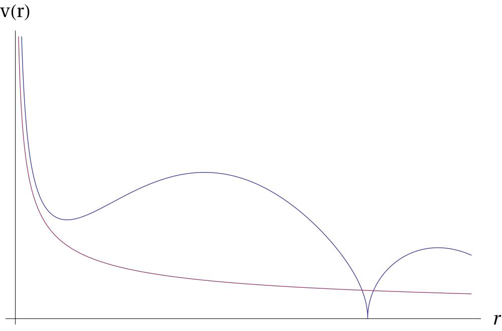
Note that these simple relations hold only outside of the mass distribution, and will be modified by the presence of mass e.g. in the halos of galaxies, and by the onset of the harmonic long-distance decay (94). The result is similar to that of an Schwarzschild-de Sitter geometry with $\Lambda_{\rm eff}$ given by (82), combined with a harmonic screening at $r\approx L_{\omega}$ . It remains to be seen if this indeed allows to explain the observed galactic rotation curves; however qualitatively, the above behavior certainly goes in the right direction. What is particularly striking is that it naturally predicts a slightly increasing rotation curve, which is indeed often observed. This may be masked by other effects, in particular the non-trivial matter distribution. In fact, the possibility that the galactic rotation curves might be explained in terms of a cosmological constant has been proposed in the literature [36]. It was argued to be feasible, provided $\Lambda_{\rm eff}$ can depend on the individual galaxy (the value $\Lambda_{\rm eff}\approx-5\times 10^{-55}cm^{-2}$ was given as a typical scale). Of course this does not make sense in conventional GR, and it is inconsistent with cosmological constraints in the $\Lambda$ CDM model. However the latter are irrelevant here as discussed below, and $G=\frac{g_{0}^{2}\omega^{4}}{\Lambda_{1}^{4}}$ is dynamical here and may indeed depend on the individual galaxy. It would be extremely interesting to study this in more detail.

Some estimates.

We certainly want to preserve $g_{00}<0$ , which implies that

1>2U_{0}=g_{0}^{2}\omega^{2}=G\frac{\Lambda_{1}^{4}}{2\omega^{2}}=\frac{\Lambda_{1}^{4}}{2\omega^{2}\Lambda_{\rm planck}^{2}}.

(95)

This allows to express the vacuum energy as

\Lambda_{1}^{2}=\sqrt{2U_{0}}\,\omega\Lambda_{\rm planck}=\sqrt{2U_{0}}\,\frac{\pi}{L_{\omega}L_{\rm planck}}

(96)

To get some idea of the scales we consider our galaxy. Assuming $L_{\omega}\approx L_{\rm galaxy}\approx 10^{20}m$ (so that the oscillations occur roughly at the size of our galaxy), this gives

\Lambda_{1}\approx U_{0}^{1/4}\,\sqrt{\frac{1}{10^{20}m10^{-35}m}}\approx U_{0}^{1/4}\,10^{7}m^{-1}\approx U_{0}^{1/4}\,10[eV].

(97)

To be specific assume that the potential energy at the center or the galaxy roughly coincides with its value given by Newtonian gravity,

U_{0}\approx MG/L_{\rm galaxy}\approx\frac{10^{15}m}{10^{20}m}\approx 10^{-5}

(98)

where $M\approx 10^{41}kg$ . Then we get a bound on $\Lambda_{1}$ of the order of electronvolt. We will see in section 4.4 that the cosmology in this model is not very sensitive to the actual value of $\Lambda_{1}$ . Moreover, $\Lambda_{4}$ could be much smaller than the Planck scale in this model as discussed below. Thus the fine-tuning is considerably milder than in the standard $\Lambda$ CDM model where $\Lambda_{1}\approx 2\times 10^{-3}eV$ .

4 General matter distribution

In this section, we generalize the above considerations to the case of an arbitrary but still somewhat localized mass distribution. The approach is a bit different from the one on the previous section, which also provides a confirmation of the above results.

Consider a large harmonic “gravity bag” solution (3.2.1) with size $L_{\omega}$ of the order of a galaxy, say, which satisfies

	$\displaystyle\phi^{i}_{0}(x,t)$	$\displaystyle=$	$\displaystyle g_{0}(x)e^{i\omega t},$
	$\displaystyle\Delta g_{0}(x)$	$\displaystyle=$	$\displaystyle-\omega^{2}g_{0}(x).$		(99)

Now add (non-relativistic) matter with $\rho(x)=\tilde{T}_{00}\geq 0$ and $\tilde{T}_{ij}\approx 0$ into this bag; indeed matter will tend to accumulate in the bag due to its attractive gravitational potential (68). If the localized matter density $\rho(x)$ (consisting of stars, etc.) is not too large, this will lead to a deformation

	$\displaystyle\phi^{i}(x,t)$	$\displaystyle=$	$\displaystyle g(x)e^{i\omega t},$
	$\displaystyle g(x)$	$\displaystyle=$	$\displaystyle g_{0}(x)+\delta g(x)$		(100)

where $|\delta g|\ll g_{0}(x)\approx g_{0}(0)$ is varying on short scales according to $\rho(x)$ , while $g_{0}(x)$ is slowly varying at the scale $L_{\omega}$ . Notice that this is precisely the splitting in (69), and the condition $|\delta g|\ll g_{0}(x)$ corresponds to (84). Thus $g_{0}(x)$ is the embedding due to the average, overall mass in the galaxy resp. the largest cosmic structures, and $\delta g(x)$ due to small local perturbations such as stars, as indicated in figure 3.

This dominance of large-scale structures is vindicated by the fact that the typical velocities of large-scale structures in cosmology are larger than for small-scale structures, cf. (93).

4.1 Metric deformation and Newtonian limit

In this situation, it makes sense to linearize in $\delta g(x)$ ; this is the crucial step. The corresponding metric is static and has the form (41)

ds^{2}=-(1-\omega^{2}\,g^{2})\,dt^{2}+(\delta_{ij}+\partial_{i}g\partial_{j}g)dx^{i}dx^{j}.

(101)

We want to derive the Poisson equation for the corresponding gravitational potential $U(x)=-\frac{1}{2}\omega^{2}g^{2}$ . Thus consider

(\Delta+\omega^{2})U=-\omega^{2}g(x)(\Delta+\omega^{2})g(x)-\omega^{2}\delta^{ij}\partial_{i}g\partial_{j}g.

(102)

Now recall the equation of motion (54)

(\Delta+\omega^{2})g=-8\pi\omega^{2}\frac{\rho}{\Lambda_{1}^{4}}g(x).

(103)

Using (99) this gives for the fluctuations

(\Delta+\omega^{2})\delta g=-8\pi\omega^{2}\frac{\rho}{\Lambda_{1}^{4}}(g_{0}+\delta g)\approx-8\pi\omega^{2}\frac{\rho}{\Lambda_{1}^{4}}\,g_{0}.

(104)

Now we use the assumption that $\rho$ is some small mass distribution inside a large background bag $g_{0}$ which is slowly varying. This means that

	$\displaystyle\partial_{i}g_{0}$	$\displaystyle=$	$\displaystyle O(r\Delta g_{0})=O(r\omega^{2}g_{0}),$
	$\displaystyle\partial_{i}\delta g$	$\displaystyle=$	$\displaystyle O(\tilde{r}\Delta\delta g)=O(\tilde{r}\omega^{2}\frac{\rho}{\Lambda_{1}^{4}}\,g_{0})$		(105)

where $r\ll L_{\omega}$ denotes the distance from the “center” of the bag, and $\tilde{r}$ is the distance from $\rho$ . Putting this together and using $\omega^{2}r^{2}\ll 1$ , we obtain

	$\displaystyle(\Delta+\omega^{2})U$	$\displaystyle=$	$\displaystyle 8\pi\omega^{4}g(x)^{2}\frac{\rho(x)}{\Lambda_{1}^{4}}-\omega^{2}\delta^{ij}\partial_{i}g\partial_{j}g$		(106)
		$\displaystyle=$	$\displaystyle 8\pi\omega^{4}g_{0}^{2}\frac{\rho(x)}{\Lambda_{1}^{4}}\,+O\Big(r^{2}\omega^{2}\omega^{4}g_{0}^{2}(1+8\pi\frac{\rho}{\Lambda_{1}^{4}})\Big)\,+O(\delta g^{2})$		(106)

This shows that the terms with first derivatives can be neglected assuming $r^{2}\omega^{2}\ll 1$ , and the term $O(\delta g^{2})$ can be neglected for small $\rho$ . Identifying the Newton constant as

G=2g_{0}^{2}\,\frac{\omega^{4}}{\Lambda_{1}^{4}},

(107)

we obtain the Poisson equation

\Delta U\approx 4\pi G\,(\rho(x)+\frac{\Lambda_{1}^{4}}{8\pi})

(108)

with an effective vacuum energy $\Lambda_{1}^{4}$ which could be interpreted as apparent negative cosmological constant $\Lambda_{\rm eff}$ . This confirms the results (81), (82) of the previous section. If the matter density is much larger than the vacuum energy,

\frac{\rho}{\Lambda_{1}^{4}}\gg 1

(109)

this gives indeed the usual Poisson equation of Newtonian gravity,

\displaystyle\Delta U

\displaystyle=

\displaystyle 4\pi G\,\rho.

(110)

As a check, consider the case of a small localized mass $M$ at the origin. The fluctuations $\delta g\ll g_{0}$ can be determined explicitly using (104), which implies $(\Delta+\omega^{2})\delta g\approx-4\pi\frac{G\rho}{g_{0}\omega^{2}}$ . Outside of the mass distribution this gives

$\displaystyle\delta g$	$\displaystyle=$	$\displaystyle g_{0}\alpha\,\frac{\sin(\omega r+\tilde{\delta})}{\omega r},$
$\displaystyle g$	$\displaystyle=$	$\displaystyle g_{0}+\delta g=g_{0}\Big(\frac{\sin(\omega r)}{\omega r}+\alpha\,\frac{\sin(\omega r+\tilde{\delta})}{\omega r}\Big)\,\approx\,g_{0}\frac{\sin(\omega r+\delta)}{\omega r},$
$\displaystyle\frac{GM}{\omega g_{0}^{2}}$	$\displaystyle=$	$\displaystyle\alpha\sin(\tilde{\delta}).$	(111)

This results in a metric which is essentially the same as (70), (71), replacing $\delta=\alpha\tilde{\delta}$ for small $\alpha$ . However, a more complete treatment including corrections due to $\theta^{\mu\nu}(x)$ and more general “gravity bags” is required before a detailed comparison with the solar system constraints can be performed.

We conclude that localized matter $\rho$ inside the gravity bag $\phi_{0}$ is subject to (emergent) Newtonian gravity, with a dynamically determined gravitational “constant” $G$ given by (107). For example, two stars or planets would lead to local perturbations

g(x)=g_{0}+\delta g_{1}(x)+\delta g_{2}(x)

(112)

where $\delta g_{i}$ are perturbations due to object $\rho_{i}$ . They both see the same $g_{0}$ and $\omega$ , thus the same gravitational constant $G$ , and Newtonian gravity is recovered on scales shorter than $L_{\omega}$ . However at very long scales $L_{\omega}$ and near the border of the galaxy, the effective gravitational constant might differ; this would require more detailed modeling.

Recall that this mechanism is necessarily non-linear and therefore somewhat non-trivial, but nevertheless it is quite robust: the essential ingredient is the gravity bag $g_{0}(x)e^{i\omega t}$ which must be slowly rotating and have large amplitude. As discussed before, it seems unavoidable that such a bag forms around large matter clusters in the static case. This leads to an effective gravity which is at least close to what we observe, and might provide an explanation for the rotational curves in typical galaxies without resorting to “dark matter”. An obvious question is how the parameters $\omega$ and $g_{0}$ , and thereby $G$ are determined; we will give an argument below why $G$ should be at least approximately the same in different galaxies.

4.2 Ricci tensor and relation with general relativity

In order to compute the Ricci tensor in the above situation, we assume for simplicity that the mass distribution $\rho$ is in the center of the background gravity bag, so that

	$\displaystyle\partial_{i}\phi_{0}$	$\displaystyle\approx$	$\displaystyle\partial_{i}g_{0}=0,$
	$\displaystyle\partial_{i}\partial_{j}g_{0}$	$\displaystyle\approx$	$\displaystyle-\frac{1}{3}\delta_{ij}\omega^{2}g_{0}$		(113)

and $g_{0}(x)\approx g_{0}-\frac{1}{6}\omega^{2}g_{0}r^{2}$ for small distances. The space-like components of the metric $h_{ij}=\partial_{i}g\partial_{j}g$ can then be written as

	$\displaystyle h_{ij}$	$\displaystyle=$	$\displaystyle\partial_{i}g_{0}\partial_{j}g_{0}+2\partial_{i}g_{0}\partial_{j}\delta g+O(\delta g^{2})$		(114)
		$\displaystyle=$	$\displaystyle\frac{1}{9}g_{0}^{2}\omega^{4}x_{i}x_{j}-\frac{2}{3}g_{0}\omega^{2}x_{i}\partial_{j}\delta g+O(\delta g^{2}).$		(114)

The Ricci tensor can be computed using the on-shell relation (55)

\partial^{\lambda}h_{\lambda\nu}=\frac{1}{2}\partial_{\nu}h+\square\phi(\partial_{\nu}\phi)=\frac{1}{2}\partial_{\nu}h-8\pi\omega^{2}\frac{\rho}{\Lambda_{1}^{4}}\phi(\partial_{\nu}\phi)

(115)

hence

\displaystyle\partial_{\mu}\partial^{\lambda}h_{\lambda\nu}

\displaystyle=

\displaystyle\frac{1}{2}\partial_{\mu}\partial_{\nu}h+\square\phi(\partial_{\mu}\partial_{\nu}\phi)+\partial_{\mu}(\square\phi)\partial_{\nu}\phi

(116)

so that

$\displaystyle R_{\mu\nu}$	$\displaystyle=$	$\displaystyle\partial_{\alpha}\Gamma^{\alpha}_{\mu\nu}-\partial_{\mu}\Gamma^{\alpha}_{\alpha\nu}=\frac{1}{2}\left(-\square h_{\mu\nu}-\partial_{\mu}\partial_{\nu}h+\partial_{\mu}\partial^{\lambda}h_{\lambda\nu}+\partial_{\nu}\partial^{\lambda}h_{\lambda\mu}\right)$
	$\displaystyle=$	$\displaystyle-(\partial_{\mu}\partial^{\lambda}\phi)(\partial_{\nu}\partial_{\lambda}\phi)+(\square\phi)(\partial_{\mu}\partial_{\nu}\phi)$
$\displaystyle R$	$\displaystyle=$	$\displaystyle-(\partial^{\mu}\partial^{\lambda}\phi)(\partial_{\mu}\partial_{\lambda}\phi)+(\square\phi)^{2}$	(117)
	$\displaystyle=$	$\displaystyle\omega^{4}g^{2}-2\omega^{2}\partial^{\lambda}\phi\partial_{\lambda}\phi-\partial^{i}\partial^{j}g\partial_{i}\partial_{j}g-(8\pi\omega^{2}\frac{\rho}{\Lambda_{1}^{4}})^{2}g^{2}$	(117)

(using $\partial_{0}\phi\partial_{0}\phi=\omega^{2}\phi^{2}=-\phi\partial_{0}^{2}\phi$ and (113)). This is hard to evaluate in general. We can write it as sum of contributions $R_{\mu\nu}=R_{\mu\nu}^{(0)}+R_{\mu\nu}^{(1)}+R_{\mu\nu}^{(2)}$ where

$\displaystyle R_{\mu\nu}^{(0)}$	$\displaystyle=$	$\displaystyle-(\partial_{\mu}\partial^{\lambda}\phi_{0})(\partial_{\nu}\partial_{\lambda}\phi_{0})$
$\displaystyle R_{\mu\nu}^{(1)}$	$\displaystyle=$	$\displaystyle-(\partial_{\mu}\partial^{\lambda}\phi_{0})(\partial_{\nu}\partial_{\lambda}\delta\phi)-(\partial_{\nu}\partial^{\lambda}\phi_{0})(\partial_{\mu}\partial_{\lambda}\delta\phi)+(\square\delta\phi)(\partial_{\mu}\partial_{\nu}\phi_{0})$
$\displaystyle R_{\mu\nu}^{(2)}$	$\displaystyle=$	$\displaystyle-(\partial_{\mu}\partial^{\lambda}\delta\phi)(\partial_{\nu}\partial_{\lambda}\delta\phi)+(\square\delta\phi)(\partial_{\mu}\partial_{\nu}\delta\phi)$	(118)

since $\square\phi_{0}=0$ . $R_{\mu\nu}^{(0)}$ is the “vacuum” contribution due to the background bag, $R_{\mu\nu}^{(1)}$ is the desired contribution due to matter linear in $\rho$ , and $R_{\mu\nu}^{(2)}=O(\rho^{2})$ is expected to be negligible for small $\rho$ . Consider first the “vacuum contribution” $R_{\mu\nu}^{(0)}$ which applies whenever $\rho=0$ :

Harmonic bag contribution.

The contribution of the harmonic bag $\phi_{0}$ is given by

R_{\mu\nu}^{(0)}=-(\partial_{\mu}\partial^{\lambda}\phi_{0})(\partial_{\nu}\partial_{\lambda}\phi_{0}),\qquad R=-(\partial^{\mu}\partial^{\lambda}\phi_{0})(\partial_{\mu}\partial_{\lambda}\phi_{0}).

(119)

This can be written using $\partial_{0}\phi\partial_{0}\phi=\omega^{2}\phi^{2}=-\phi\partial_{0}^{2}\phi$ and (113) as

$\displaystyle R_{00}$	$\displaystyle=$	$\displaystyle-\omega^{2}\partial^{\lambda}\phi_{0}\partial_{\lambda}\phi_{0}\approx-\omega^{4}g_{0}^{2}=-\frac{1}{2}G\Lambda_{1}^{4},$
$\displaystyle R_{ij}$	$\displaystyle=$	$\displaystyle-(\partial_{i}\partial_{k}\phi_{0})(\partial_{j}\partial_{k}\phi_{0})\approx-\frac{1}{9}\delta_{ij}\omega^{4}g_{0}^{2}=-\frac{1}{18}\delta_{ij}G\Lambda_{1}^{4}$
$\displaystyle R$	$\displaystyle\approx$	$\displaystyle\frac{2}{3}\omega^{4}g_{0}^{2}=\frac{1}{3}G\Lambda_{1}^{4}.$	(120)

Therefore $R_{\mu\nu}^{(0)}=O(G\Lambda_{1}^{4})$ as expected, and

	$\displaystyle{\cal G}_{00}$	$\displaystyle=$	$\displaystyle R_{00}-\frac{1}{2}\eta_{00}R=-\frac{1}{3}G\Lambda_{1}^{4},$
	$\displaystyle{\cal G}_{ij}$	$\displaystyle=$	$\displaystyle R_{ij}-\frac{1}{2}\delta_{ij}R=-\frac{2}{9}\delta_{ij}G\Lambda_{1}^{4}.$		(121)

In the presence of some local matter distributions $\rho(x)$ , this background will be dominated by the gravitational field due to $\rho(x)$ . This is contained in $R_{\mu\nu}^{(1)}$ which we compute next.

Linear matter contribution.

Now consider $R_{\mu\nu}^{(1)}$ , which is the desired contribution linear in $\rho$ . To proceed we consider the time-and space-like components separately:

$\displaystyle R_{00}$	$\displaystyle=$	$\displaystyle-2\omega^{2}\partial^{\lambda}\phi_{0}\partial_{\lambda}\delta\phi+8\pi\omega^{4}g_{0}^{2}\frac{\rho}{\Lambda_{1}^{4}}$	(122)
	$\displaystyle=$	$\displaystyle-2\omega^{4}g_{0}\delta g+8\pi\omega^{4}g_{0}^{2}\frac{\rho}{\Lambda_{1}^{4}}\approx 4\pi G\rho+2U(x)\omega^{2}$
	$\displaystyle\approx$	$\displaystyle 4\pi G\rho$

where $U(x)$ is the gravitational potential due to $\rho$ as determined earlier; that term is negligible since $4\pi G\rho\approx\Delta U(x)\gg U(x)\omega^{2}$ by assumption. This is in agreement with GR as discussed below. $R_{0i}=0$ follows again from $\partial_{0}\phi\partial_{i}\phi=0$ , and

$\displaystyle R_{ij}$	$\displaystyle=$	$\displaystyle-(\partial_{\mu}\partial^{\lambda}\phi_{0})(\partial_{\nu}\partial_{\lambda}\delta\phi)-(\partial_{j}\partial^{\lambda}\phi)(\partial_{i}\partial_{\lambda}\delta\phi)-8\pi\omega^{2}\frac{\rho}{\Lambda_{1}^{4}}g_{0}\partial_{i}\partial_{j}g_{0}$	(123)
	$\displaystyle\approx$	$\displaystyle-(\partial_{i}\partial_{k}g_{0})(\partial_{j}\partial_{k}\delta g)-(\partial_{j}\partial_{k}g_{0})(\partial_{i}\partial_{k}\delta g)-8\pi\omega^{2}\frac{\rho}{\Lambda_{1}^{4}}g_{0}\partial_{i}\partial_{j}g_{0}$
	$\displaystyle\approx$	$\displaystyle\frac{2}{3}\omega^{2}g_{0}\partial_{j}\partial_{i}\delta g+\frac{1}{3}4\pi G\rho\delta_{ij}$

using (113). This gives

\displaystyle R

\displaystyle=

\displaystyle-4\pi G\rho+\frac{2}{3}\omega^{2}g_{0}\Delta\delta g+4\pi G\rho=-\frac{2}{3}4\pi G\rho

(124)

and

	$\displaystyle{\cal G}_{00}$	$\displaystyle=$	$\displaystyle R_{00}-\frac{1}{2}\eta_{00}R=\frac{2}{3}8\pi G\rho,$
	$\displaystyle{\cal G}_{ij}$	$\displaystyle=$	$\displaystyle R_{ij}-\frac{1}{2}\delta_{ij}R\approx\frac{2}{3}\omega^{2}g_{0}\partial_{j}\partial_{i}\delta g+\frac{2}{3}4\pi G\rho\delta_{ij}.$		(125)

In particular, in regions where $\rho(x)=0$ we obtain indeed

{\cal G}_{00}=R_{00}=GT_{00}=0,\quad R=0

(126)

as in GR, up to corrections due to the vacuum energy. Recall that in GR, the Einstein equations for $T^{00}=\rho,\,\,T^{ij}=0$ imply ${\cal G}_{00}=8\pi G\rho$ , and furthermore $R_{ij}=4\pi g_{ij}G\rho,\,\,R_{00}=4\pi G\rho$ and $8\pi G\rho=R$ . Thus (122) and (126) agree with GR, while the space-like (pressure) components of $R_{ij}$ and ${\cal G}_{ij}$ are different here from GR. In particular, for $\rho=0$ the essential difference to GR is an anisotropy of $R_{ij}$ . Indeed we should not expect complete agreement with GR since there are no harmonic embeddings of non-trivial Ricci-flat 4-manifolds [37].

The non-vanishing components of ${\cal G}^{ij}=O(G\rho)$ would endanger the Newtonian limit if indeed $\Lambda_{4}=\Lambda_{\rm planck}$ . On the other hand, this does not pose any problem if $\Lambda_{4}\ll\Lambda_{\rm planck}$ , so that the contributions of $\Lambda_{4}^{2}{\cal G}^{ij}$ are negligible. This scenario is quite possible and in fact very appealing as discussed below, greatly reducing the required fine-tuning for $\Lambda_{1}$ .

4.3 Quantization, scales and stability

Perhaps the most remarkable result is that gravity arises in the harmonic branch of the matrix model, without even using the induced gravitational action i.e. the Einstein-Hilbert term. This means that the scale $\Lambda_{4}$ in front of the induced Einstein-Hilbert term (42) could be much smaller than the Planck scale,

\Lambda_{4}\ll\Lambda_{\rm planck}

(127)

because the Newton constant $G$ is determined dynamically through (81). In principle, $\Lambda_{4}$ might be as low as $O(TeV)$ ¹⁶¹⁶ 16 A similar possibility has also been considered in [9] however in a rather different context of higher-dimensional GR with branes.. In fact this should be so in the present context, since otherwise the non-vanishing components ${\cal G}_{ij}$ found above would enter equation (47) and might spoil the results of the previous sections (unless they vanish in a more sophisticated solution). This is of course a very attractive scenario, because then the difference of scales between $\Lambda_{1}$ and $\Lambda_{4}$ would be greatly reduced, largely resolving the cosmological constant problem.

Another extremely interesting feature of the harmonic branch of the model is that the quantization of gravity seems to be straight-forward and well-behaved. Indeed $\Lambda_{4}$ is essentially the scale of $N=4$ SUSY breaking, and the model can be viewed as non-commutative $N=4$ SYM on ${\mathbb{R}}^{4}_{\theta}$ which is expected to provide a well-defined quantum theory. The degrees of freedom in $\theta^{\mu\nu}(x)$ can be interpreted as would-be $U(1)$ non-commutative gauge fields on ${\mathbb{R}}^{4}_{\theta}$ , which are also well-behaved in the IKKT model. The excitations of the scalar fields $\phi_{i}$ are essentially harmonic excitations due to the brane tension/vacuum energy

S_{\rm vac}=-2\Lambda_{1}^{4}\int d^{4}x\sqrt{|g|}\approx-\Lambda_{1}^{4}\int d^{4}x(2+\eta^{\mu\nu}\partial_{\mu}\phi^{i}\partial_{\nu}\phi^{j}\delta_{ij})

(128)

with positive energy

E_{\rm vac}\approx\Lambda_{1}^{4}\int d^{3}x\,(2+\partial_{0}\phi\partial_{0}\phi+\partial_{i}\phi\partial_{i}\phi\delta^{ij}).

(129)

This is similar to the quantization of a Klein-Gordon field. Note in particular that the energy of the gravity bags is proportional to $g_{0}^{2}\omega^{2}$ , hence its scale is more-or-less determined dynamically by the initial energy distribution. In particular, it is plausible that the total energy of the universe consisting of brane fluctuations and the total mass is positive. This suggests that also after structure formation, the (vacuum) energy of the gravity bags associated to a galaxy with mass $M$ should be no less than its gravitational binding energy $MU$ . Then increasing $g_{0}$ would increase the total energy, which is important for stability reasons.

In contrast, many of the difficulties associated with the quantization of GR are expected to be recovered in the Einstein branch of the model.

It remains to be seen whether the emergent gravity is compatible with the precise solar system constraints, which requires a more complete analysis. Finally it should be pointed out that the considerations of this paper should be extended to cover the case of small extra dimensions, e.g. in the form of fuzzy sphere(s). The basic results of this paper are expected to apply also in that case.

4.4 Cosmological context and perturbations

We briefly explain how the above solutions fit into a consistent cosmology. Assuming that the vacuum energy $\Lambda_{1}^{4}$ dominates the energy density due to matter, cosmological solutions of emergent NC gravity were obtained in [11] as harmonically embedded branes ${\cal M}^{4}\subset{\mathbb{R}}^{10}$

\vec{x}(t,\chi,\theta,\varphi)=\left(\begin{array}[]{c}{\cal R}(t)\left(\begin{array}[]{l}\sinh(\chi)\sin\theta\cos\varphi\\ \sinh(\chi)\sin\theta\sin\varphi\\ \sinh(\chi)\cos\theta\\ \cosh(\chi)\end{array}\right)\\ 0\\ x_{c}(t)\end{array}\right)\in{\mathbb{R}}^{10}

where

{\cal R}(t)=a(t)\,\left(\begin{array}[]{l}\cos\psi(t)\\ \sin\psi(t)\end{array}\right).

(130)

Here $\eta_{ab}=\mbox{diag}(+,...+,-,-,+,+)$ for $k=-1$ . This embedding is harmonic, $\Delta_{g}\vec{x}=0$ , and has a FRW geometry

ds^{2}=-dt^{2}+a(t)^{2}d\Sigma^{2},\qquad d\Sigma^{2}=d\chi^{2}+\sinh^{2}(\chi)d\Omega^{2}

(131)

corresponding to spatial curvature $k=-1$ . The physics of the early universe in this model is quite different from standard cosmology and requires a more detailed analysis¹⁷¹⁷ 17 In particular the consistency with the CMB data cannot be reliably addressed at this point, see however [38] for the simplified case of an exact Milne universe. The above refined solutions yield a big bounce and an early phase with power-law acceleration [11], but a proper treatment of matter is still missing.; however, it is a solid prediction that the solution approaches $a(t)\to t$ for late times, i.e. a Milne universe. Remarkably, this geometry is in good agreement with the basic observational data including the tye Ia supernovae data [38], which are usually interpreted in terms of an accelerating universe.

Milne universe.

The Milne geometry is expected to hold in this model as long as the vacuum energy $\Lambda_{1}^{4}$ dominates the energy density due to matter. In particular, there is no upper bound on $\Lambda_{1}$ from cosmology. These statements are easy to understand, recalling that the Milne universe is nothing but (a sector of) flat Minkowski space ${\mathbb{R}}^{4}\subset{\mathbb{R}}^{10}$ . Indeed consider the flat metric $ds^{2}=-d\tau^{2}+dr^{2}+r^{2}d\Omega^{2}$ on ${\mathbb{R}}^{4}$ . In terms of the new variables

\tau=t\cosh(\chi),\,\,r=t\sinh(\chi),

(132)

this metric takes the form of a FRW metric with $a(t)=t$ and $k=-1$ ,

	$\displaystyle ds^{2}_{g}$	$\displaystyle=$	$\displaystyle-d\tau^{2}+dr^{2}+r^{2}d\Omega^{2}=\frac{a^{2}}{\tilde{t}^{2}}\left(-dt^{2}+t^{2}(d\chi^{2}+\sinh^{2}(\chi)d\Omega^{2})\right)$		(133)
		$\displaystyle=$	$\displaystyle-dt^{2}+a(t)^{2}(d\chi^{2}+\sinh^{2}(\chi)d\Omega^{2}).$		(133)

Clearly, flat Minkowski space is a solution of a brane with tension resp. vacuum energy $\sim\Lambda_{1}^{4}$ , and in fact it is stabilized by a large $\Lambda_{1}$ .

We claim that matter such as stars and galaxies lead to local perturbations resp. fluctuations of this cosmological solution, and the previous results including Newtonian gravity and long-distance deviations go through with very minor adaptation. This can be seen easily by using the previous localized solutions on ${\mathbb{R}}^{4}$ and rewriting them in terms of the Milne variables. For example, the spherically symmetric solutions centered at the origin $r=\chi=0$ become

$\displaystyle\phi_{0}(x)$	$\displaystyle=$	$\displaystyle g(r)e^{i\omega\tau}=g_{0}\frac{\sin(\omega r)}{\omega r}e^{i\omega\tau}$	(134)
	$\displaystyle=$	$\displaystyle g_{0}\frac{\sin(\omega t\sinh(\chi))}{\omega t\sinh(\chi)}e^{i\omega\cosh(\chi)t}$
	$\displaystyle\approx$	$\displaystyle g_{0}\frac{\sin(\omega a(t)\chi)}{\omega a(t)\chi}e^{i\omega t}$

using $\chi\ll 1$ in the neighborhood of the mass. Thus in comoving Milne coordinates, this looks like a spherically symmetric solution with red-shifted wavelength $a(t)\omega=t\omega$ . Note that the effective gravitational constant $G=\frac{2g_{0}^{2}\omega^{4}}{\Lambda_{1}^{4}}$ is independent of $t$ , which is reassuring¹⁸¹⁸ 18 $G$ might change in the very early universe due to deviations from the Milne metric.. A particularly interesting aspect is the slow “extrinsic” rotation (130) in the embedding ${\cal M}\subset{\mathbb{R}}^{D}$ for small $t$ , which turns out to be [11]

\dot{\psi}\sim\frac{1}{a^{5}}.

(135)

This might be very important in the context of fluctuation spectra in the early universe. Clearly a more complete perturbation analysis is required, in particular in order to address the issues of fluctuation spectra in the context of the cosmic microwave background.

We can thus summarize the physical aspects of the model as follows, leaving aside its theoretical appeal e.g. with respect to quantization. The most attractive feature of the model is that it naturally predicts a (nearly-) flat universe, resulting in luminosity curves e.g. for type Ia supernovae which are close to the observed ones (usually interpreted in terms of cosmic acceleration) without any fine-tuning. On the other hand, reconciling it with observed gravity on scales less than or equal to galactic scales does impose an upper bound on the vacuum energy of order eV. This in turn might offer a mechanism for (partially?) explaining the galactic rotation curves, without requiring large amounts of dark matter.

Gravitational (non–)constant $G$ .

Up to now, the parameters $\omega,g_{0}$ and therefore $G$ were undetermined. However these are dynamical quantities, in particular they depend on the initial conditions. Thus we have to face the question why in particular $G$ should be the same in different parts of the universe, in particular in different galaxies. Indeed one should expect in this model that $G$ depends somewhat on the individual galaxies, however the variation should certainly not be too large in our universe.

While we cannot offer a completely satisfactory answer yet, some insight can be obtained from the above cosmological solutions. We have seen that deformations $g(x)$ of the brane due to e.g. galaxies can be considered as perturbations propagating in an approximately flat Milne resp. Minkowski background, with $\omega$ and $g_{0}$ remaining essentially constant in time. In reality, we know that galaxies are typically parts of larger structures such as (super)-clusters and filaments. This large-scale structure is expected to provide the dominant contribution to $g(x)$ and therefore to $G$ , which is therefore related over cosmological scales. Moreover, it is very plausible that the dynamics of structure formation in the universe leads to similar scales for $g_{0}(x)$ of these dominant cosmic structures, given the high degree of homogeneity of the initial conditions seen in the CMB background. Furthermore, the rotation $\dot{\psi}$ of the above cosmological solution (130) might provide a natural seed for the required rotation of the large-scale gravity bags. On the other hand, there could be some other more rigid mechanism for stabilizing $G$ which we did not identify here.

5 Discussion

We obtained in this paper some remarkable results on the long-distance properties of emergent gravity in Yang-Mills matrix models, notably the IKKT model. Space-time is modeled by a 3+1-dimensional noncommutative brane solution, which acquires an “emergent” metric. Its dynamics is governed by the brane tension as well as additional gravitational terms including the Einstein- Hilbert term in the (quantum) effective action. There are two types of gravitational solution: an “Einstein branch” which is very similar to general relativity, and a “harmonic branch” where the branes are governed by a brane tension. We focus on the harmonic branch in this paper, and study the deformation of the space-time brane and its effective metric due to static localized mass distributions, having in mind e.g. galaxies.

Due to the brane tension, the basic excitations of the space-time brane are essentially harmonic waves. Large matter clusters such as galaxies are embedded in such “gravity bags”, which are rotating standing waves of the embedding with long wavelength $L_{\omega}$ . Standard Newtonian gravity is recovered inside these “gravity bags” due to local matter such as stars. Moreover, there is an effective gravitational constant $\Lambda_{\rm eff}$ inside the bags, which leads to a significant enhancement of orbital velocities at large distances, quite reminiscent of the observed galactic rotation curves. At very large distances $\geq L_{\omega}$ , the harmonic embedding leads to a screening $\sim\frac{1}{r^{2}}$ of the gravitational potential, reconciling relatively large vacuum energies (of order $eV$ , say) with a consistent cosmology similar to a Milne universe. The latter is known to be in remarkably good agreement with the basic cosmological constraints, leaving aside the CMB fluctuations which require a detailed understanding of the early universe in this model.

These results have important physical implications. An obvious conjecture is that the observed enhancement of the galactic rotation velocities compared with the Newtonian law is primarily due to the above results, i.e. an effective vacuum energy $\Lambda_{\rm eff}$ inside the gravity bags. This gets additional support by the result that the gravitational constant $G$ and therefore $\Lambda_{\rm eff}$ is not universal but determined dynamically, and may therefore differ somewhat from galaxy to galaxy. This does not imply that there is no dark matter at all, but the model clearly requires far less dark matter in the galactic halos than what is invoked in the $\Lambda$ CDM model.

It is certainly remarkable how close this simple and rigid model comes to observation. In particular, large-scale cosmological observations seem to be reproduced much more naturally in the harmonic branch than in GR, without particular fine-tuning of the vacuum energy. The basic solar system observations can be reproduced to a good approximation, which seems to require an upper bound on $\Lambda_{\rm eff}$ on the order of $eV$ . However, the precision tests provide a challenge, and it remains to be seen whether they can be met in the harmonic branch of solutions under consideration. The only obvious modifications of the matrix model would be quadratic or cubic (soft) terms, which do not spoil the good UV behavior of its quantization. The cubic terms lead to compactified extra dimensions as fuzzy spheres, which is very natural and desirable for particle physics [39]. The quadratic terms might help to stabilizes the “scale” of space-time resp. the effective vacuum energy. Indeed observational constraints require that the vacuum energy is quite small (perhaps $O(eV)$ ). This may be due to a cancellation between the bare action and the induced quantum-mechanical vacuum energy, but quadratic terms in the matrix model might also play an important role here.

Another remarkable feature of the model is that gravity is naturally weak. Indeed the scale of gravity is found to be $G\sim\frac{g_{0}^{2}}{L_{\omega}^{4}\Lambda_{1}^{4}}$ , where $L_{\omega}$ is a cosmological length scale, and $\Lambda_{1}$ the vacuum energy. Moreover $G$ can differ to some extent in different parts of the universe, and depends on the surrounding mass distribution which determines a “gravity bag”.

In any case, an essential result of this paper is that Newtonian gravity arises in the matrix model simply due to the brane tension of a harmonically embedded space-time brane; the Einstein-Hilbert action is not required. This suggest the following very appealing scenario: the coefficient $\Lambda_{4}^{2}$ of the induced Einstein-Hilbert term could be much smaller than the Planck scale. This would also greatly alleviate the fine-tuning issue for the vacuum energy, and the precise form of the (induced) gravitational action is not essential. This basic mechanism might apply in a more general framework than that of Yang-Mills matrix models. However, the matrix model offers a clear concept of quantization, in particular the IKKT model. It contains not only (emergent) gravity but all ingredients required for a theory of fundamental interactions, in particular nonabelian gauge fields and fermions. This would provide a very interesting and accessible quantum theory of gravity, which has the potential to resolve some fundamental problems in this context.

There are many obvious shortcomings in this paper which require more detailed work. The present understanding is still at a rather crude level, and more detailed work is needed before claiming to seriously challenge the $\Lambda$ CDM model. Probably the main problem are the space-like components of ${\cal G}^{\mu\nu}$ resp. $g_{rr}$ , which do not quite agree with GR even in vacuum. It remains to be seen if the solutions presented here can meet the solar system precision tests, or if a more complete solution taking into account notably $\theta^{\mu\nu}(x)$ will lead to the suitable corrections. Furthermore, the short-distance properties of a point-mass solution i.e. black holes should be studied in the matrix model framework. Here higher-order corrections due to $\theta^{\mu\nu}$ are expected to play an important role. Finally, the Einstein branch of the IKKT model should provide a quantization of more conventional general relativity coupled to matter.

Acknowledgments

The author wishes to thank in particular N. Arkani-Hamed for very useful discussions and hospitality at the IAS Princeton, as well as R. Brandenberger, G. Dvali, H. Grosse, D. Klammer, H. Rumpf and I. Sachs for useful discussions, and the CERN theory division for hospitality. This work was supported in part by the FWF project P20017 and in part by the FWF project P21610.

References

[1] N. Ishibashi, H. Kawai, Y. Kitazawa and A. Tsuchiya, “A large-N reduced model as superstring,” Nucl. Phys. B 498 (1997) 467 [arXiv:hep-th/9612115].
[2] H. Steinacker, “Emergent Gravity from Noncommutative Gauge Theory,” JHEP 12, (2007) 049; [arXiv:0708.2426 [hep-th]].
[3] H. Steinacker, “Emergent Gravity and Noncommutative Branes from Yang-Mills Matrix Models,” Nucl. Phys. B 810:1-39,2009. arXiv:0806.2032 [hep-th].
[4] H. Steinacker, “Covariant Field Equations, Gauge Fields and Conservation Laws from Yang-Mills Matrix Models,” JHEP 0902 (2009) 044 [arXiv:0812.3761 [hep-th]].
[5] V. O. Rivelles, “Noncommutative field theories and gravity,” Phys. Lett. B 558 (2003) 191 [arXiv:hep-th/0212262].
[6] H. S. Yang, “Emergent gravity from noncommutative spacetime,” arXiv:hep-th/0611174; H. S. Yang, “On The Correspondence Between Noncommuative Field Theory And Gravity,” Mod. Phys. Lett. A 22 (2007) 1119 [arXiv:hep-th/0612231].
[7] H. S. Yang, “Emergent Spacetime and The Origin of Gravity,” arXiv:0809.4728 [hep-th]; H. S. Yang and M. Sivakumar, “Emergent Gravity from Quantized Spacetime,” arXiv:0908.2809 [hep-th].
[8] B. Muthukumar, “U(1) gauge invariant noncommutative Schroedinger theory and gravity,” Phys. Rev. D 71, 105007 (2005) [arXiv:hep-th/0412069]; A. H. Fatollahi, “Particle Dynamics And Emergent Gravity,” arXiv:0805.1159 [hep-th].
[9] N. Arkani-Hamed, S. Dimopoulos and G. R. Dvali, “The hierarchy problem and new dimensions at a millimeter,” Phys. Lett. B 429 (1998) 263 [arXiv:hep-ph/9803315].
[10] G. R. Dvali, G. Gabadadze and M. Porrati, “4D gravity on a brane in 5D Minkowski space,” Phys. Lett. B 485 (2000) 208 [arXiv:hep-th/0005016].
[11] D. Klammer and H. Steinacker, “Cosmological solutions of emergent noncommutative gravity,” Phys. Rev. Lett. 102 (2009) 221301 [arXiv:0903.0986 [gr-qc]].
[12] T. Banks, N. Seiberg and S. H. Shenker, “Branes from matrices,” Nucl. Phys. B 490 (1997) 91 [arXiv:hep-th/9612157].
[13] V. P. Nair and S. Randjbar-Daemi, “On brane solutions in M(atrix) theory,” Nucl. Phys. B 533 (1998) 333 [arXiv:hep-th/9802187].
[14] H. Aoki, N. Ishibashi, S. Iso, H. Kawai, Y. Kitazawa and T. Tada, “Noncommutative Yang-Mills in IIB matrix model,” Nucl. Phys. B 565 (2000) 176 [arXiv:hep-th/9908141].
[15] I. Chepelev, Y. Makeenko and K. Zarembo, “Properties of D-branes in matrix model of IIB superstring,” Phys. Lett. B 400 (1997) 43 [arXiv:hep-th/9701151].
[16] M.R. Douglas and N.A. Nekrasov, “Noncommutative Field Theory”, Rev. Mod. Phys. 73 (2001) 977–1029 [hep-th/0106048].
[17] R.J. Szabo, “Quantum Field Theory on Noncommutative Spaces”, Phys. Rept. 378 (2003) 207–299 [hep-th/0109162]; R. J. Szabo, “Quantum Gravity, Field Theory and Signatures of Noncommutative Spacetime,” arXiv:0906.2913 [hep-th].
[18] A. Y. Alekseev, A. Recknagel and V. Schomerus, “Brane dynamics in background fluxes and non-commutative geometry,” JHEP 0005 (2000) 010 [arXiv:hep-th/0003187].
[19] M. Chaichian, A. Tureanu, R. B. Zhang and X. Zhang, “Riemannian geometry of noncommutative surfaces,” J. Math. Phys. 49 (2008) 073511 [arXiv:hep-th/0612128].
[20] J. Madore, S. Schraml, P. Schupp and J. Wess, “Gauge theory on noncommutative spaces,” Eur. Phys. J. C 16 (2000) 161 [arXiv:hep-th/0001203].
[21] N. Seiberg and E. Witten, “String theory and noncommutative geometry,” JHEP 9909 (1999) 032 [arXiv:hep-th/9908142].
[22] W. Taylor, “M(atrix) theory: Matrix quantum mechanics as a fundamental theory,” Rev. Mod. Phys. 73 (2001) 419 [arXiv:hep-th/0101126]; D. Kabat and W. I. Taylor, “Linearized supergravity from matrix theory,” Phys. Lett. B 426 (1998) 297 [arXiv:hep-th/9712185];
[23] T. Banks, W. Fischler, S. H. Shenker and L. Susskind, “M theory as a matrix model: A conjecture,” Phys. Rev. D 55 (1997) 5112 [arXiv:hep-th/9610043].
[24] H. Aoki, S. Iso, H. Kawai, Y. Kitazawa and T. Tada, “Space-time structures from IIB matrix model,” Prog. Theor. Phys. 99 (1998) 713 [arXiv:hep-th/9802085].
[25] Y. Kitazawa and S. Nagaoka, “Graviton propagators in supergravity and noncommutative gauge theory,” Phys. Rev. D 75, 046007 (2007) [arXiv:hep-th/0611056]; Y. Kitazawa and S. Nagaoka, “Graviton propagators on fuzzy G/H,” JHEP 0602 (2006) 001 [arXiv:hep-th/0512204].
[26] J. Nishimura and F. Sugino, “Dynamical generation of four-dimensional space-time in the IIB matrix model,” JHEP 0205 (2002) 001 [arXiv:hep-th/0111102]. J. Nishimura and G. Vernizzi, “Spontaneous breakdown of Lorentz invariance in IIB matrix model,” JHEP 0004 (2000) 015 [arXiv:hep-th/0003223].
[27] H. Nicolai and R. Helling, “Supermembranes and M(atrix) theory,” arXiv:hep-th/9809103.
[28] B. de Wit, J. Hoppe and H. Nicolai, “On the quantum mechanics of supermembranes,” Nucl. Phys. B 305 (1988) 545.
[29] J. Madore, “The fuzzy sphere,” Class. Quant. Grav. 9, 69 (1992).
[30] S. Liberati, F. Girelli and L. Sindoni, “Analogue Models for Emergent Gravity,” arXiv:0909.3834 [gr-qc].
[31] A. Matusis, L. Susskind and N. Toumbas, “The IR/UV connection in the non-commutative gauge theories,” JHEP 0012 (2000) 002 [arXiv:hep-th/0002075].
[32] H. Grosse, H. Steinacker and M. Wohlgenannt, “Emergent Gravity, Matrix Models and UV/IR Mixing,” JHEP 0804 (2008) 023 [arXiv:0802.0973 [hep-th]];
[33] C.J.S. Clarke, “On the Global Isometric Embedding of Pseudo-Riemannian Manifolds”, Proc. Royal Soc. London, A 314, 417 (1970)
[34] D. Klammer and H. Steinacker, “Fermions and Emergent Noncommutative Gravity,” JHEP 0808 (2008) 074 [arXiv:0805.1157 [hep-th]]
[35] W. Rindler, “Relativity: Special, General, And Cosmological,” Oxford, UK: Univ. Pr. (2006) 430 p
[36] S. B. Whitehouse and G. V. Kraniotis, “A possible explanation of Galactic Velocity Rotation Curves in terms of a Cosmological Constant,” arXiv:astro-ph/9911485.
[37] B. Nielsen, “Minimal Immersions, Einstein’s Equations and Mach’s Principle”. Jour. Geom. Phys. bf 4, no. 1, 1 (1987)
[38] A. Benoit-Levy and G. Chardin, “Do we live in a ’Dirac-Milne’ universe?,” arXiv:0903.2446 [astro-ph.CO]; G. Sethi, A. Dev and D. Jain, “Cosmological Constraints on a Power Law Universe,” Phys. Lett. B 624 (2005) 135 [arXiv:astro-ph/0506255].
[39] P. Aschieri, T. Grammatikopoulos, H. Steinacker and G. Zoupanos, “Dynamical generation of fuzzy extra dimensions, dimensional reduction and symmetry breaking,” JHEP 0609 (2006) 026 [arXiv:hep-th/0606021].

On the Newtonian limit of emergent NC gravity and long-distance corrections