Littelmann patterns and Weyl group multiple Dirichlet series of type $D$Thanks: We thank Ben Brubaker and Sol Friedberg for helpful conversations. Both authors thank the NSF for support

We begin with some notation. Let $\Phi$ be a reduced root system of rank $r$ and $n$ a positive integer. Let $F$ be a number field containing the $2n$-th roots of unity. Let $S$ be a set of places of $F$ containing the archimedean places and those that ramify over $\mathbb{Q}$, as well as sufficiently many more places to ensure that the ring of $S$-integers $\mathcal{O}_{S}$ has class number $1$. Let $\mathbf{m}=(m_{1},\dotsc,m_{r})$ be a fixed nonzero tuple of elements of $\mathcal{O}_{S}$. Let $\mathbf{s}=(s_{1},\dotsc,s_{r})$ be an $r$-tuple of complex variables.

Given the data above, one can form a Weyl group multiple Dirichlet series. This is a Dirichlet series in the $r$ variables $s_{i}$ with a group of functional equations isomorphic to the Weyl group $W$ of $\Phi$. More precisely, one can define a set of functions of the form

where each $c_{i}$ ranges over nonzero elements of $\mathcal{O}_{S}$ modulo units, ${\it\Psi}$ is taken from a certain finite-dimensional complex vector space $\Omega$ of functions on $(F_{S}^{\times})^{r}$, and $H$ is an important function we shall say more about shortly. Then the collection of all such $Z$ as ${\it\Psi}$ ranges over a basis of $\Omega$ satisfies a group of functional equations isomorphic to $W$ with an appropriate scattering matrix. For more about why Weyl group multiple Dirichlet series are interesting objects, as well as a discussion about the basic framework for their construction, we refer to [6].

The heart of the construction of $Z$ is the function $H$. This function must be carefully defined to ensure that $Z$ satisfies the correct group of functional equations. The heuristic of [6] dictates how to define $H$ on the powerfree tuples $\mathbf{c},\mathbf{m}$ (those tuples such that the product $c_{1}\dotsb c_{r}m_{1}\dotsb m_{r}$ is squarefree). Moreover, it is further specified in [6] how the values of $H$ on the prime power tuples $\mathbf{c}=(\varpi^{k_{1}},\dotsc,\varpi^{k_{r}})$, $\mathbf{m}=(\varpi^{l_{1}},\dotsc,\varpi^{l_{r}})$, where $\varpi\in\mathcal{O}_{S}$ is a prime, determine $H$ on all tuples.

Thus, writing $\ell$ for a tuple of nonnegative integers $(l_{1},\dotsc,l_{r})$ and letting $\varpi^{\ell}$ denote the tuple $(\varpi^{l_{1}},\dotsc,\varpi^{l_{r}})$, the construction of $Z$ reduces to understanding the multivariate generating function

At present there are two different approaches to understanding the generating function (1), and thus to constructing Weyl group multiple Dirichlet series. Both are related to characters of representations of the semisimple complex Lie algebra attached to $\Phi$. Let $\omega_{i},i=1,\dotsc,r$ be the fundamental weights of $\Phi$ and let $\theta$ be the strictly dominant weight $\sum(l_{i}+{1})\omega_{i}$.

• •

  The Gelfand–Tsetlin approach [3, 5, 2], which works for $\Phi=A_{r}$, gives formulas for the coefficients $H(\varpi^{k_{1}},\dotsc,\varpi^{k_{r}};\varpi^{\ell})$. These formulas are written in terms of Gauss sums and statistics extracted from Gelfand–Tsetlin patterns for the representation of $\fSL_{r+1}(\mathbb{C})$ of lowest weight $-\theta$.

• •

  The averaging approach [10, 12, 8, 9], which works for all $\Phi$, uses a “metaplectic” deformation of the Weyl character formula to construct a rational function with known denominator, whose numerator is then taken to define $N$.

Both approaches have their advantages and limitations. The Gelfand–Tsetlin construction gives very explicit formulas for $H$, formulas that (remarkably) are uniform in $n$ and that lead to a direct connection with the global Fourier coefficients of Borel Eisenstein series on the $n$-fold cover of $\SL_{r+1}$ [1], but suffers from the obvious disadvantage that it only works for type $A$. The averaging approach, on the other hand, works for all $\Phi$, quickly leads to the definition of $Z$, yet has the drawback that it seems difficult to get similarly explicit formulas for the coefficients of $N$. By combining recent work of Chinta–Offen [11] and McNamara [14], we know that in type $A$ the two definitions of $N$ coincide, although it seems difficult to give a direct combinatorial proof.

This note arose from our attempts to understand the Gelfand–Tsetlin approach to (1). In the course of studying [3], it became plain to us that the most suitable language to understand the constructions in [3] is that of Kashiwara’s crystal graphs, as encoded in the generalization of the Gelfand–Tsetlin basis due to Littelmann [13], which we call Littelmann patterns. Indeed, the definitions in [3] become much more transparent when phrased in terms of these patterns.

To test the relevance of this observation, we decided to try to formulate a Littelmann analogue of the Gelfand–Tsetlin construction when $\Phi$ is a root system of type $D$. The main result of this note is thus Conjecture 1, which explicitly describes the generating function $N(x_{1},\dotsc,x_{r};\ell)$ for the $\varpi$-part of the type $D$ Weyl group multiple Dirichlet series constructed using the averaging method. We remark that for $n=1$, Conjecture 1 gives a type $D$ analogue of a theorem of Tokuyama [15].

We have some limited evidence for the truth of Conjecture 1.

First, for $D_{2}\simeq A_{1}\times A_{1}$, the conjecture is easily seen to be true.

Next, we have tested the conjecture for $D_{3}$ when $n\leq 4$ and for $D_{4}$ when $n\leq 2$, by computing the $\varpi$-parts by averaging for many tuples $\ell$ and comparing with the predictions of Conjecture 1. In all cases there was complete agreement. Note that $D_{3}\simeq A_{3}$, so the $\varpi$-part of the $D_{3}$-series has already been described explicitly using the results of [3], and in this guise has already been compared extensively with $\varpi$-parts constructed by averaging. Nevertheless, agreement in rank $3$ between $\varpi$-parts constructed using Conjecture 1 and using averaging is a nontrivial check, since $D_{3}$ Littelmann patterns are quite different from $A_{3}$ Gelfand–Tsetlin patterns.

Finally, recently Brubaker and Friedberg have computed the global Whittaker coefficients of Eisenstein series on covers of $\GL_{4}$ by inducing from the parabolic subgroup of type $\GL_{2}\times\GL_{2}$ [4]. Their computations—which build on earlier work of Bump–Hoffstein [7] and are the first attempts to extend the results of [1] beyond type $A$ and to work with other parabolic subgroups—express the Whittaker coefficients in terms of certain exponential sums. In the course of their work Brubaker and Friedberg found that the integrals can be broken up in accordance with the decomposition of $H(\varpi^{k_{1}},\dotsc,\varpi^{k_{r}};\varpi^{\ell})$ given by Conjecture 1, and that if one does so the contributions to the global Whittaker coefficient exactly agrees with Conjecture 1. We find this connection between Eisenstein series and $\varpi$-parts to be strongly convincing evidence of the correctness of Conjecture 1.

Let $\mathfrak{g}$ be the simple complex Lie algebra of type $D_{r}$, in other words the Lie algebra of the group $\SO_{2r}(\mathbb{C})$. Let $\theta$ be a dominant weight of $\mathfrak{g}$ and let $V_{\theta}$ be the irreducible $\mathfrak{g}$-module of highest weight $\theta$. In [13, §7] Littelmann describes a way to index a basis of $V_{\theta}$ using patterns that are analogous to the classical Gelfand–Tsetlin patterns for the Lie algebra of $\SL_{r}(\mathbb{C})$. In this section we recall his construction.

First we label vertices of the Dynkin diagram of $\mathfrak{g}$ with the integers $1,\dotsc,r$. We label the upper node of the right prong $1$, the lower node of the prong $2$, the node at the elbow of the prong $3$, and then the remaining nodes increase from $4$ to $r$, reading right to left (Figure 1). We remark that this is not the standard labelling by Bourbaki, which begins with $1$ at the left of the diagram.

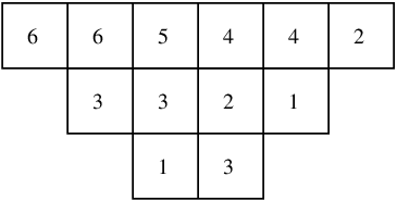
A pattern $T$ for $D_{r}$ consists of a collection of integers $a_{i,j}$, where $1\leq i\leq r-1$ and $i\leq j\leq 2r-2$. We picture $T$ by drawing the integers placed in $r-1$ rows of centered boxes. The first row contains $2r-2$ boxes, the second $2r-4$ boxes, and so on down to the $(r-1)$-st row, which contains $2$ boxes. The integers are placed in the boxes so that $a_{i,i}$ is placed in the leftmost box of the $i$th row, and then the remaining integers $a_{i,j}$ are put in the boxes in order as $j$ increases. We define an involution on each row by $\overline{a}_{i,j}=a_{i,2r-1-j}$.

To index a weight vector in $V_{\theta}$, there are two sets of inequalities the $a_{i,j}$ must satisfy. The first is independent of $\theta$: in each row we must have

or, using the bar notation,

In other words, the $a_{i,j}$ are weakly decreasing in the rows, with the exception that no comparison is made between $a_{i,r-1}$ and $a_{i,r}$. Both of these entries, however, are required to be $\leq a_{i,r-2}$ and $\geq a_{i,r+1}$.

Figure 2 shows an admissible pattern for $D_{4}$.

The next set of inequalities involves the highest weight $\theta$. Write

where the $\omega_{k}$ are the fundamental weights. Then an admissible $T$ will correspond to a weight vector in $V_{\theta}$ if $T$ satisfies

where we write for $j<r-1$

Note that the inequalities for the $i$th row only involve the entries of $T$ on the $i$th and $(i-1)$st rows. Moreover when ordered in terms of increasing $i$, there is a unique inequality in which a given entry $a_{i,j}$ appears on the left.

To complete our discussion of Littelmann patterns, we must assign a weight $\lambda(T)$ to each pattern $T$. This is a vector $\lambda(T)=(\lambda_{1},\dotsc,\lambda_{r})$ of nonnegative integers, where

We write $|\lambda|=\lambda_{1}+\dotsb+\lambda_{r}$. In our conjecture, if a pattern $T$ occurs for the twist $\theta=\sum m_{i}\omega_{i}$, it will contribute to the coefficient of $\mathbf{x}^{\lambda(T)}:=x_{1}^{\lambda_{1}}\dotsb x_{r}^{\lambda_{r}}$ in the numerator $N(\mathbf{x},\ell)$, where $\ell=(l_{1},\dotsc,l_{r})$ and $l_{i}=m_{i}-1$. For instance, the pattern in Figure 2 contributes to the coefficient of $x_{1}^{9}x_{2}^{9}x_{3}^{14}x_{4}^{8}$, with $x_{1}$ corresponding to left middle column of three entries and $x_{2}$ to the right middle column of three entries.

Let $T$ be a $\theta$-admissible pattern. We want to associate to $T$ a graph $\Gamma(T)$. The graph $\Gamma(T)$ will also potentially be endowed with decorations, which will be circled vertices. The vertices of $\Gamma(T)$ correspond to the entries of $T$; the graph will have at least one connected component for each row of $T$.

We begin by describing how each row determines a subgraph. Consider the $i$th row of $T$. Each entry $a_{i,j}$ in this row gives an vertex. We draw the corresponding vertices in a row, with the two vertices in the middle corresponding to the incomparable entries $a_{i,r-1},a_{i,r}$ entries arranged vertically. For definiteness we assign $a_{i,r-1}$ to the top vertex and $a_{i,r}$ to the bottom vertex. See Figure 3 for the arrangement for the top row of a pattern for $D_{6}$.

Now join two vertices by an edge if they appear consecutively in the inequalities (2), are equal, and are comparable in (2). Note that we do not join the vertices corresponding to $a_{i,r-1},a_{i,r}$ by an edge if they happen to be equal, since they are not comparable in (2). This gives a graph for this row. We then do the same for each row of $T$. The result is $\Gamma(T)$ without decorations.

Certain symmetric connected components that arise in the construction of $\Gamma(T)$ will play a special role in our conjecture:

The term leaning is inspired by [3]; see also §5. Figure 4 shows an example of a symmetric multiple leaner of length $5$, when all the entries in the top row of a pattern for $D_{6}$ are equal. Note that the minimal length of a symmetric multiple leaner is $2$, and that multiple leaners can appear in patterns for $D_{3}$, but not for $D_{2}$.

To complete the construction of $\Gamma(T)$ we must describe how to add the decorations. This is very simple: we circle each vertex whose corresponding entry is critical in the sense of Definition 3.

Figure 5 shows an example of building the decorated graph of the Littelmann pattern in Figure 2. We assume that a highest weight $\theta$ has been specified so that the circled vertices in the graph correspond to critical entries.

In the following for $k=1,\dotsc,n-1$ we write $g_{k}$ for the Gauss sum $g(\varpi^{k-1},\varpi^{k})$ (see for example [8] for the definition of the Gauss sums). For convenience we extend the notation and define $g_{0}$ to be $-1$. It is also convenient to define $g_{m}$ for $m\geq n$ by $g_{m}=g_{k}$, where $m=k$ mod $n$ and $k=0,\dots,n-1$. We let $p$ be the norm of $\varpi$.

In [3] certain patterns for a given weight are discarded and do not contribute to the relevant coefficient of $N$; such patterns are called strict in [3]. In type $A$ strictness corresponds to an easily stated property for Gelfand–Tsetlin patterns. If one interprets the definition of strictness in [3] in terms of type $A$ Littelmann patterns, one sees that a type $A$ pattern is nonstrict exactly when

• •

  an entry is simultaneously $0$ and critical, or

• •

  there are two adjacent entries that are equal, with the left entry critical.

We take these to be our definition for type $D$ patterns as well:

Note that the subgraph from Figure 6 is allowed to appear in multiple-leaners.

Let $T$ be a strict pattern, and let $\Gamma(T)$ be the associated decorated graph. For any connected component $C$ of $\Gamma(T)$, let $y_{C}$ be the rightmost vertex, in the sense of the order induced by the inequalities (2). If $C$ has two rightmost vertices, meaning that it is in the $i$-th row and contains entries $a_{i,r-2}=a_{i,r-1}=a_{i,r}\not=a_{i,r+1}$, then we define the rightmost vertex to be the vertex corresponding to $a_{i,r-1}$, that is, the upper vertex in Figure 3.

We are almost ready to state our conjecture. There is one more phenomenon that plays a role, namely leaning. Essentially, leaning means that if entries are consecutive and equal in a Littelmann pattern $T$, where consecutive means adjacent in (2), then only one should contribute to the corresponding coefficient of $N(\mathbf{x};\ell)$. This is why we introduce the graph $\Gamma(T)$. Its connected components keep track of these equalities among entries.

Thus we are led to consider contributions of the connected components of $\Gamma(T)$, not just the entries. There is further slight twist that the contribution of a multiple leaning component is different from that of all other components:

We are now ready to state our conjecture: