Relativistic Euler’s 3-body problem,
optical geometry and the golden ratio
Abstract
A Weyl solution describing two Schwarzschild black holes is considered. We focus on the invariant solution, with ADM mass , where is the Komar mass of each black hole. For this solution the set of fixed points of the discrete symmetry is a totally geodesic sub-manifold. The existence and radii of circular photon orbits in this sub-manifold are studied, as functions of the distance between the two black holes. For there are two such orbits, corresponding to and in Schwarzschild coordinates. As the distance increases, it is shown that the two photon orbits approach one another and merge when , where is the golden ratio. Beyond this distance there exist no circular photon orbits. The two null orbits delimit a forbidden band for time-like circular orbits, which is interpreted in terms of optical geometry. For large , time-like circular orbits are allowed everywhere, as in the analogous Newtonian problem. The analysis is generalised by considering a invariant Weyl solution with an array of black holes and also by charging the black holes, which connects the Weyl solution to a Majumdar-Papapetrou spacetime.
1 Introduction
Euler’s 3-body problem is a soluble special case of the general 3-body problem, in which a test particle moves in the gravitational field of two gravitational sources - point masses - which are fixed in space. It is Liouville integrable since, besides the energy and one component of the angular momentum, there is a third constant of the motion (see e.g. [1, 2]; see [3] for a hyperbolic space version of the problem which is still integrable). A natural relativistic generalisation of this problem is to consider the motion of test particles in a Weyl solution describing two Schwarzschild black holes, which are kept in equilibrium due to a strut in between them. For this problem there is no known analogue to Euler’s constant (see [4] for a discussion about this point); equivalently, there is no known separability for the geodesic equations. Generic geodesics have, therefore, to be studied numerically. For the special case in which the two black holes have equal mass, there is, however, a 1+2 dimensional totally geodesic sub-manifold in which geodesics are Liouville integrable. In particular it is straightforward to derive all circular causal orbits.
Regular (on and outside an event horizon) static black holes in vacuum general relativity do not admit causal circular geodesics below a certain critical radius, which lies outside the event horizon. Below this radius, the angular momentum term in the radial equation of motion, usually centrifugal (with respect to the black hole), becomes centripetal, making equilibrium impossible. This change in character of the angular momentum term has a geometric interpretation in terms of optical geometry [5]: define “outwards” as the direction in which fixed points sets of the optical geometry’s isometry group (spheres) increase their proper size; then, the angular momentum term is always “outwards”. Similar considerations may be made about stationary black holes. However, in this case the optical geometry is a Randers-Finsler rather than Riemannian geometry, making the interpretation more subtle [6].
In this paper we show that the optical geometry of the aforementioned relativistic Euler’s 3-body problem is richer than the standard one of the Schwarzschild black hole. To be concrete let the two black holes in the Weyl solution considered have equal mass and separation between them. This choice of masses implies that there is a discrete symmetry of the solution. The set of fixed points of this discrete symmetry is a totally geodesic sub-manifold, . The optical geometry of this sub-manifold then has the following feature: for sufficiently small but non-zero the notion of “outwards”, defined as above, changes continuously twice, rather than just once. This means that, on , there is an annulus-like region in which ”outwards” means a decreasing radial Weyl canonical coordinate. The boundaries of this annular region are the loci of two circular photon orbits, and the region itself is a forbidden band for time-like circular geodesics, which are allowed everywhere outside this band. As increases, the two boundaries of the annular region approach one another and coalesce when , where is the golden ratio! For larger , admits no circular photon orbits and time-like circular geodesics are allowed everywhere, just as in the symmetric Euler’s 3-body problem.
Considering a Weyl solution with an array of , rather than two, black holes along a line, still possessing a discrete symmetry, leads to two cases. For even (odd), we essentially recover the optical geometry of the () case. We shall also consider charged black holes in Einstein-Maxwell theory, by using a solution generating technique [10] that allows the introduction of a charge parameter in Weyl solutions. For black holes, the charge parameter is the ratio of charge to mass, which is the same for all the black holes in the solution. In this case, as we increase the charge for fixed , the proper area of the forbidden band increases; for , this area diverges as we reach extremality, as a consequence of the infinite ‘throat’ developed by extremal black holes. Keeping the charge and fixed, the area of the forbidden band decreases as is increased, just as for the uncharged case, becoming zero at some maximum value of .
This paper is organised as follows. After a brief discussion of the Newtonian Euler’s 3-body problem in section 2, we describe in section 3.1 the Weyl solutions that shall be used in the relativistic version of the problem, as well as the circular null and time-like orbits. In section 3.2 the charged case is considered. In section 4 the interpretation of the forbidden band for time-like circular orbits is given in terms of optical geometry. In section 5 we briefly discuss the case of multiple black holes. We close with some final remarks.
2 The Newtonian version
In Euler’s 3-body problem, a.k.a. the two-centre Kepler problem (see e.g. [7]), with both masses equal to , the motion of a test particle moving in the symmetry plane between the two masses obeys
| (1) |
where is a radial cylindrical coordinate, are the energy and angular momentum per unit mass and is the distance from either mass to the symmetry plane. We shall use geometrised units throughout. Circular orbits are seen by extremising the potential. They obey
| (2) |
This equation has solution for any , given and . The angular momentum goes to zero (infinity) as () - Fig. 1. Thus circular orbits exist for any radial distance in the symmetry plane. This is therefore the behaviour we expect in the relativistic version of the problem for large , and indeed it is the behaviour we shall find. The behaviour for small will, however, be quite different.

In the relativistic problem that shall be considered in the next section, the Newtonian gravitational potential of one or multiple rods (rather than point-like masses) of mass , infinitesimal width and mass density plays an important role, since it is a key ingredient in the construction of Weyl solutions describing one or multiple black holes. Let us remark that, as a Newtonian problem, the passage from point particles to two equal rods, aligned with the direction of separation, does not alter the previous conclusion: in the symmetry plane, circular orbits still exist at any radial distance from the symmetry axis.
3 The relativistic version
3.1 Uncharged case
Weyl geometries [8, 9] in four space-time dimensions admit two commuting, mutually orthogonal Killing vector fields. In vacuum, the metric may always be written in the form
| (3) |
The vacuum Einstein equations, , reduce to a harmonic equation in an auxiliary Euclidean three space, , in cylindrical coordinates ,
| (4) |
and two partial differential equations for
| (5) |
which become line integrals once the solution for is known.
A solution with two black holes is obtained by taking to be the potential of two finite rods of zero width and linear density .11 1 This particular choice is required to avoid curvature singularities at the rod positions. The rods are placed at and in the intervals and . Then
| (6) |
where we have introduced the quantities
| (7) |
Introducing further
| (8) |
the solution of (5), given (6), is
| (9) |
An integration constant could be added to . We have chosen this constant to be zero. With this choice, identifying the azimuthal coordinate with standard period , the metric is smooth, on the symmetry axis for and . For and there is a conical excess, given by
| (10) |
The vacuum solution described by (3), (6) and (9) is actually a three parameters family of solutions. Physically, the three parameters may be taken to be the two black holes masses and the distance between them. The black hole masses may be computed as Komar integrals:
| (11) |
where is the dual 1-form to the time-like Killing vector field and the 2-surfaces correspond to the location of the two finite rods in Weyl coordinates. An asymptotic expansion shows that the ADM mass is
| (12) |
For the distance we shall take the coordinate distance in Weyl coordinates
| (13) |
This is a monotonic function of the proper distance
| (14) |
and hence a good measure thereof.
In order to have a totally geodesic sub-manifold we require . We also choose a symmetric coordinate system: and . The proper distance between the two black holes may then be expressed as
| (15) |
where is a complete elliptic integral of the second kind. It follows that is a totally geodesic sub-manifold, which has induced metric given by (3) with . Geodesics in this sub-manifold obey
| (16) |
where the dot represents derivative with respect to an affine parameter and we have introduced the energy and angular momentum for a particle of mass .
3.1.1 Circular photon orbits
From (16), circular null geodesics are determined by the extrema of the potential
| (17) |
For , i.e the single black hole limit, making the coordinate transformation
| (18) |
the potential becomes
| (19) |
This is the effective potential for photons in a Schwarzschild black hole and in Schwarzschild coordinates. It has the well known extremum at . Another solution for a constant photon orbit is , corresponding to the null geodesic generator of the horizon. Thus, in Weyl coordinates we have two extrema, for , at
| (20) |
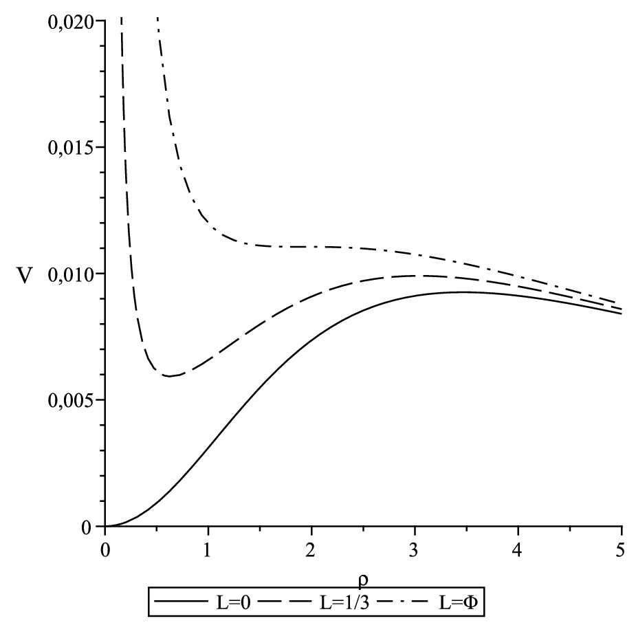
For , has no extrema, since it is approximately . The interpolation between these two behaviours is as follows - Fig 2. As grows, the two extrema (20) approach one another, in both coordinate and proper distance, and merge for . Beyond this value of , has no extrema. To see the value of , observe that the extrema of (17) are given by
| (21) |
To solve for it is convenient to introduce and . Then the last equation becomes
| (22) |
Take (22) to define a curve , between and ; at these values of , . These two “points” of the curve correspond to and given in (20). Constant slices of the curve have two solutions for , one solution for and no solution for . To determine , it is convenient to introduce
| (23) |
Then, differentiating (22), extremising and replacing back into (22) gives the quadratic equation
| (24) |
whose only solution leading to a positive is
| (25) |
is the golden ratio. Using the recurrence property of the golden ratio
| (26) |
we arrive at , and therefore at
| (27) |
where is the golden ratio conjugate. Thus, quite strikingly, the two null circular orbits merge when the ratio between the Komar mass of either black hole and the semi-distance between them is the golden ratio! This merging happens for Weyl radial coordinate
| (28) |

3.1.2 Circular time-like orbits
The significance of the circular photon orbits described in the last subsection can be seen by considering circular time-like orbits. From (16) these are obtained by extremising the potential
| (29) | |||||
where is now the angular momentum per unit mass. The extrema of this potential are given by
| (30) |
In Fig. 3 we display the solution of Eq. (30) for , in terms of , for fixed values of . One observes that for there is a forbidden band for time-like circular geodesics, which is the region between the two photon circular orbits. This behaviour should be contrasted with that exhibited in Fig. 1 for the Newtonian case and is illustrated in Fig. 4.


3.2 Charged case
Let us start by recalling that in a Reissner-Nordström black hole, the circular null orbits are found as extrema of the potential
| (31) |
in standard Schwarzschild-type coordinates, where is the charge to mass ratio of the black hole. Extremising this potential gives the location of the circular null orbit outside the horizon
| (32) |
whereas the second null orbit, with constant radial coordinate, relevant for our analysis is located at the horizon
| (33) |
Thus, the forbidden band for circular time-like orbits exists for all black holes in the Reissner-Nordström family. In the extremal case, this band acquires the special property of having infinite area, since the horizon, at , is at an infinite proper radial distance from any point with radial coordinate , which is the case for .
In order to consider two charged Reissner-Nordström black holes we shall now discuss charged Weyl solutions. The background fields are
| (34) |
The electrovacuum Einstein-Maxwell equations
| (35) |
give rise to the set of equations
| (36) |
and
| (37) |
This set of equations is more involved than eq. (4)-(5), in particular because there is no longer a linear equation to be solved. However, if one takes
| (38) |
where is a constant, and
| (39) |
the Einstein-Maxwell equations for (34) reduce to exactly the eq. (4)-(5) [10]. Thus we take and to be the same as in the uncharged case, (6) and (9). The background (34) will then describe a double Reissner-Nordström solution, wherein both black holes have the same charge to mass ratio .
The study of circular null geodesics will follow that of the uncharged case, mutatis mutandis; they will be given by the extrema of the potential
| (40) |
where may be read off from (17). Such extrema obey
| (41) |
where
| (42) |

The result for the radii of the photon circular orbits in terms of the distance for various values of the charge is shown in Fig. 5, where we used the coordinate . The first feature we wish to emphasise is that, as is increased for fixed charge, the two photon orbits approach one another, just as for the uncharged case, and coalesce for a maximum value of . Thus, the forbidden band for time-like circular orbits exists for all possible values of the charge, for sufficiently small . The second feature we want to mention is that, fixing and increasing the charge, the forbidden band has larger area. For this area diverges as extremality is approached, as mentioned above. In Fig. 6 we exhibit an example with .
In the extremal case, for which the solution is completely regular on and outside the event horizon, the analysis may also be done using the Majumdar-Papapetrou [11, 12] form of the solution:
| (43) |
where
| (44) |
In this extremal case, circular null orbits exist in the sub-manifold as long as the equation
| (45) |
has solutions for real and positive , which for fixed is possible when obeys
| (46) |

4 Interpretation: Optical Geometry
A dimensional static geometry with isometry group may always be expressed by the line element
| (47) |
where is the line element on the -sphere. The optical geometry is the effective spatial geometry seen by light rays:
| (48) |
defined where .
For the spacetime (47), the radial equation of motion of a particle with mass, energy and angular momentum , respectively is
| (49) |
Circular null orbits are therefore determined by the extrema of the potential
| (50) |
which is both the coefficient of the angular momentum term in (49) and the inverse of the proper radius squared of the sphere line element in the optical geometry. This potential pushes the test particle in the direction of increasing proper size of the spheres in the optical geometry. We dub this direction as outwards. If it coincides with our naïve notion of “outwards”, the angular momentum term may still be interpreted as a centrifugal term, as in flat space. Time-like circular orbits are only possible in a region where this term and the mass term in (49) originate forces in opposite directions.
For a single Schwarzschild black hole of mass , circular time-like orbits are possible for in Schwarzschild coordinates. Thus they are forbidden, outside the horizon, for . In this case, the optical geometry is
| (51) |
The proper size (area) of the 2-sphere is therefore , where the potential is given by (19). The area increases with for , but decreases for - Fig. 7 (left). Thus the “centrifugal force” points towards the black hole, for . Since the mass term is always attractive towards the black hole, there can be no circular time-like orbits in the region .


For the double Schwarzschild solution the optical geometry in the symmetry plane is
| (52) |
The proper size (perimeter) of the circle is therefore given by , where the potential is given by (17). The forbidden band for circular time-like orbits is the region wherein the radial coordinate decreases “outwards”, and therefore, the “centrifugal force” becomes directed to the symmetry axis - Fig. 7 (right) - preventing again the existence of time-like circular orbits.
5 Multiple black holes
We shall now consider a Weyl solution with uncharged black holes. Then (6) is replaced by
| (53) |
This function describes the Newtonian potential of rods of infinitesimal width and mass density , located at and with coordinate in the intervals, respectively,
| (54) |
Imposing
| (55) |
the geometry still admits a discrete symmetry, of which is a fixed point set. Then, the circular null orbits in this totally geodesic sub-manifold are obtained by extremising the potential
| (56) |
which yields the condition
| (57) |
We set
| (58) |
such that the coordinate distance between each two black holes is and their Komar mass is . In Fig. 8 we have plotted the radial coordinate of circular null orbits versus , for various numbers of black holes. For even, the behaviour is quite similar to that discussed for . Moreover
| (59) |
For odd, the behaviour is quite similar to that of a single Schwarzschild black hole, due to the existence of a black hole in the symmetry plane.


6 Final Remarks
In this paper we have studied a relativistic version of Euler’s 3-body problem: the motion of test particles in a invariant Weyl solution describing two (or more) black holes. We have considered both uncharged and charged black holes, within Einstein-Maxwell theory. Generically, these solutions have conical singularities on the symmetry axis. In the extremal case, however, they become a special case of the Majumdar-Papapetrou spacetimes, and are completely regular on and outside the event horizon [13, 14].
For sufficiently small distance between the two black holes, there are two circular null geodesics in the symmetry plane corresponding to the set of fixed points of the symmetry. The interior one is stable (against perturbations in the symmetry plane), while the exterior one is unstable. These orbits delimit a forbidden region for circular time-like geodesics. In the optical geometry, the proper size of the isometry group orbits grows towards the symmetry axis, rather than away from it, in this region. This unusual property is correlated with a physical effect that may be, heuristically, described as the centrifugal force becoming directed towards the symmetry axis. Thus, it cannot balance the gravitational attraction, preventing the existence of time-like circular orbits.
The existence of a stable circular null geodesic is associated with a behaviour which may be described as an ‘optical fibre’ or ‘wave guide’ like geometry. Photons with sufficiently low energy will be caught in a potential well in the radial direction, as may be observed in Fig. 2. Thus, as they move in the direction, photons will oscillate between a maximum and a minimum radii. The wave guide like geometry may allow light waves to travel around the direction without decreasing their amplitude significantly.22 2 In a very different context, this resembles the SOFAR (Sound Fixing and Ranging) channel [15], in the ocean, which occurs at the depth where the sound velocity is minimal, and allows the singing of whales to travel very long distances [16].
As the distance between the two black holes is increased, the two null circular orbits approach one another, eventually coalescing. For the uncharged case this happens when the ratio between the Komar mass of each black hole and the semi-distance between the black holes is the golden ratio.
One may ask whether the geodesic equations in the full spacetime, rather than just the symmetry plane, are Liouville integrable. In [17] a similar question was studied for extremal black holes in Einstein-Maxwell-dilaton theory, for arbitrary dilaton coupling. These authors showed that the geodesic motion is generically chaotic. There is only a very special case of integrable motion: when the dilaton coupling is that of Kaluza-Klein theory. For the generic case studied herein, of charged Weyl solutions that may be continuously connected to the extremal black holes of Einstein-Maxwell theory (with zero dilaton coupling therefore), it seems quite unlikely that the motion may be integrable. Observe however, that the uncharged double Schwarzschild solution may also be continuously connected to the extremal black holes of Kaluza-Klein theory. Thus, it would be interesting to understand where, along this trajectory in the space of solutions, integrability appears.
Acknowledgments
We are very grateful to G. W. Gibbons and E. Teo for correspondence and comments on drafts of this paper. F.C. is supported by a junior research grant from Centro de Física do Porto. C.H. is supported by a Ciência 2007 research contract. This work as been further supported by the FCT grant CERN/FP/83508/2008.
References
- [1] C. A. Coulson and A. Joseph, “A constant of the motion for the two-centre Kepler problem,” Int. Jour. Quant. Chem. 1 (1967) 337.
- [2] D. Lynden-Bell, “A simple derivation and interpretation of the third integral in stellar dynamics,” Mon. Not. R. Astron. Soc. 338 (2003) 208.
- [3] G. W. Gibbons and C. M. Warnick, “Hidden symmetry of hyperbolic monopole motion,” J. Geom. Phys. 57 (2007) 2286 [arXiv:hep-th/0609051].
- [4] C. M. Will, “Carter-like constants of the motion in Newtonian gravity and electrodynamics,” Phys. Rev. Lett. 102 (2009) 061101 [arXiv:0812.0110 [gr-qc]].
- [5] M. A. Abramowicz, “Black Holes and the Centrifugal Force Paradox,” Scientific American, March 1993, 74-81.
- [6] G. W. Gibbons, C. A. R. Herdeiro, C. M. Warnick and M. C. Werner, “Stationary Metrics and Optical Zermelo-Randers-Finsler Geometry,” Phys. Rev. D 79 (2009) 044022 [arXiv:0811.2877 [gr-qc]].
- [7] J. V. José and E. J. Saletan, “Classical Dynamics (a contemporary approach),” Cambridge University Press, 1998.
- [8] H. Weyl, Ann. Phys. (Leipzig) 54 (1917) 117.
- [9] H. Stephani et al., “Exact Solutions of Einstein’s Field Equations,” Cambridge Monographs on Mathematical Physics, 2003.
- [10] T. Azuma and T. Koikawa, “Equilibrium condition in the axisymmetric N-Reissner-Nordstrom solution,” Prog. Theor. Phys. 92 (1994) 1095.
- [11] S. D. Majumdar, Phys. Rev. 72 (1947) 390.
- [12] A. Papapetrou, Proc. R. Irish Acad. A51 (1947) 191.
- [13] J. B. Hartle and S. W. Hawking, “Solutions of the Einstein-Maxwell equations with many black holes,” Commun. Math. Phys. 26 (1972) 87.
- [14] G. W. Gibbons, “Non-Existence Of Equilibrium Configurations Of Charged Black Holes,” Proc. Roy. Soc. Lond. A 372 (1980) 535.
- [15] G. W. Gibbons, Private communication.
- [16] C. S. Morawetz, “Geometrical Optics and the singing of whales,” The Amer. Math. Mon. 85 (1978) 548.
- [17] N. J. Cornish and G. W. Gibbons, “The tale of two centres,” Class. Quant. Grav. 14 (1997) 1865 [arXiv:gr-qc/9612060].