Optimization of large homogeneous Air Cherenkov Arrays and application to the design of a 1TeV-100TeV -ray observatory.
Abstract
At the time large air Cherenkov arrays are being discussed for future -ray observatories, we review the relationship between the targeted capabilities and the main design parameters taking into account construction costs. As an example application, we describe a telescope array optimized for observations between 1 TeV and a few 100 TeV and use detailed simulations to estimate its performances in comparison to science objectives.
1 Introduction
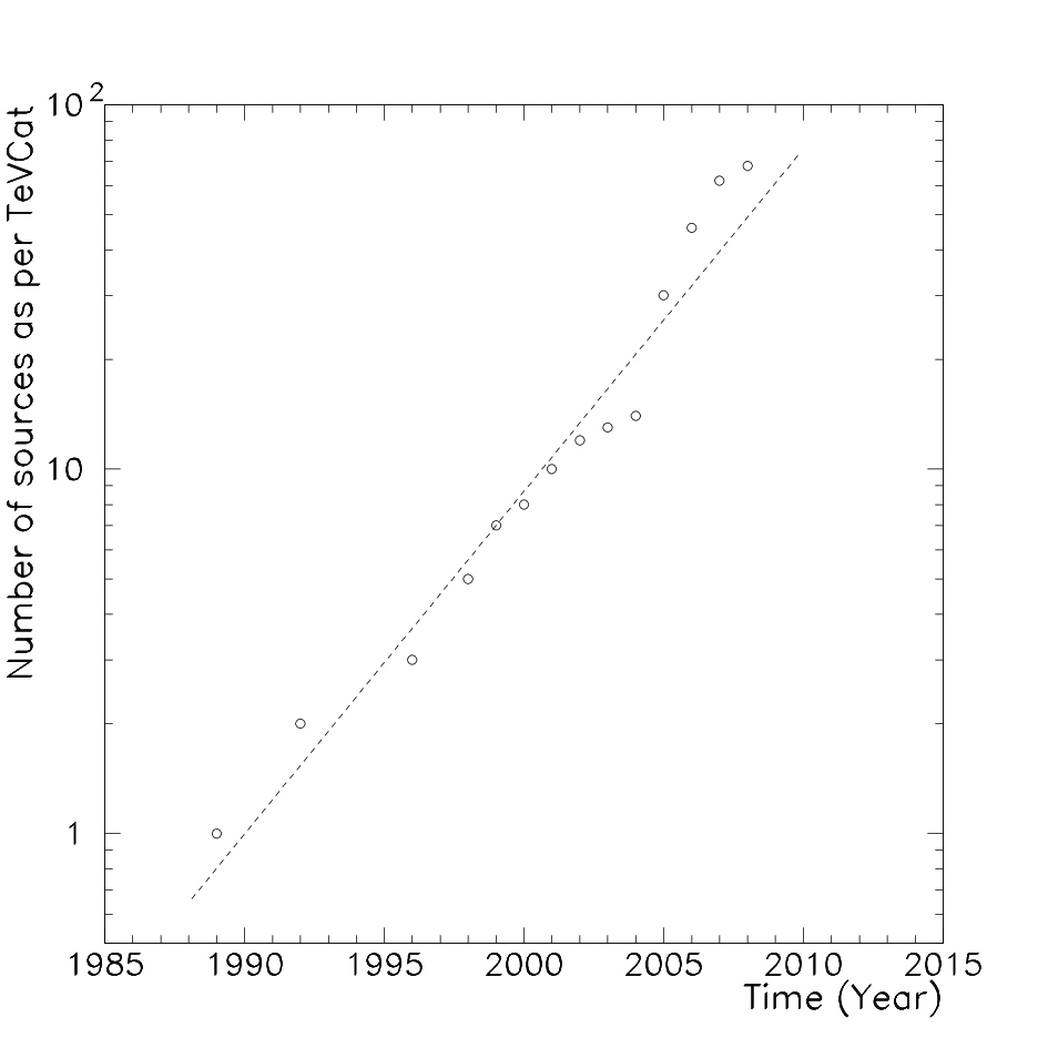
Gamma-ray astronomy at more than has entered a phase of explosive development as illustrated in Figure 1 which shows a source count doubling time just a little larger than 3 years. Possibly more interesting than the net number of sources is the diversity in the nature of objects found to produce Very High Energy (VHE) radiation. The VHE -ray sky now counts various flavors of Active Galactic Nuclei, X-ray binaries, shell type supernova remnants, pulsar wind nebulae, a pulsar, galactic diffuse emission, star forming regions and a plethora of sources that still have to be identified [1]. For the most part, these recent successes resulted from the deployment of Imaging Air Cherenkov Telescope (IACT) arrays which provide the highest angular resolution and instantaneous sensitivity at these energies. This motivates the world-wide ongoing efforts toward the construction of new large IACT arrays designed to achieve one order of magnitude improvement in sensitivity while broadening energy range coverage. IACT arrays now in operation count from 2 to 4 large telescopes and the targeted sensitivity improvement implies much larger facilities which have to be carefully optimized to obtain a maximal science capability out of always limited budgets.
In this paper, we discuss the optimization of a uniform IACT array and, as an example, we present an array to concentrate on the 1 TeV-100 TeV energy range. In section 2 we present considerations for the design and optimization of an array based on the properties of the atmospheric Cherenkov radiation emitted by VHE -ray air showers. This can be used to draw prescriptions for large IACT-array main design parameters given the energy range and collection area to be achieved while minimizing costs. In section 3 we discuss the benefits from improving sensitivity at energies greater than 1 TeV and present the performance requirements to effectively extend -ray astronomy to 100 TeV. This motivates the design of the example IACT array presented and characterized in section 4 with detailed simulations.
2 Considerations for the design of IACT arrays
2.1 Design and performance key parameters
The design of an IACT array should be driven by the science objectives and the corresponding performances to be achieved. The primary capabilities of a telescope array are the -ray effective collection area, the cosmic-ray (CR) background rejection performance and the angular resolution over the covered energy range and effective field of view. In great part and in various ways, this sets the sensitivity of the observatory. These performance characteristics are related to the array-design parameters in a way that depends on the properties of the atmospheric -ray-shower Cherenkov radiation as investigated here. In order to limit the number of design parameters, we chose to restrict our study to arrays made of a single type of telescopes, uniformly distributed on a periodic lattice, and using identical homogeneous cameras. The study remains applicable to observatories made of several homogeneous sub-arrays specialized in different energy bands for example. The primary design parameters defining such homogeneous arrays are: the number of telescopes, , the elementary-cell shape, the inter-telescope distance, , the light-collector diameter, , the field of view, , and the pixel size, . The overall photodetection efficiency (including the mirror reflectivity, light cone efficiency, photodetector quantum efficiency, etc.) could be also added in this list but it is generally technology limited and cannot be considered as a real free parameter. Moreover, an increase in photodetection efficiency would result in the same improvement as a corresponding increase in the telescope diameter, thus, can be regarded as an effective telescope diameter.
All performances of an array can not realistically be addressed with precision without detailed simulations such as presented in section 4 for an example array. Exploiting geometrical considerations and the properties of the atmospheric Cherenkov light from VHE -ray showers, it is however possible to identify relationships between the energy range (), the effective collection area, , and the design parameters of a uniform telescope array. These relations can serve as guidelines in the design of IACT arrays. There is nevertheless not a one to one relation between performance and design parameters. An external constraint must be used to make a choice and that constraint is most likely of financial nature. For that reason, after exploring the connections between design and performances, we will consider cost issues to obtain a prescription for the design of large IACT arrays. In this process, we assume a minimal number of telescope participating in an event is required for a good reconstruction, but we ignore the possible dependences of -ray/CR discrimination and angular resolution on other design parameters that can realistically be addressed only with detailed simulation of the instruments.
2.2 Effective collection area and Array foot-print
Stereoscopic observation with IACT has proven to be the best technique to reconstruct the direction and energy of primary rays. This technique relies on multiple views of a single shower from several positions on the ground. Without considering any specific properties of the atmospheric Cherenkov light, it is clear that stereoscopic reconstruction requires the shower axis to be at a distance from the telescopes that is not too large compared to the inter-telescope distance. Hence the effective area of a large IACT array is larger but close to the geometrical area covered by the array foot-print.

In an homogeneous array, the choice of the elementary cell shape affects how large an area a -telescope array covers. Using the inter-telescope distance as a unit, Figure 2 (left) shows the distribution of the distance from the shower axis to the closest three telescopes inside hexagonal and square arrays respectively. The effective collection area at a given energy depends on the maximal distance, , guarantying a single-telescope detection and on the minimal number of telescope required to participate in an event. For a given (We will later investigate how this distance arises), the effective area scales as as long as is much smaller than . For larger , the full geometrical area may not be effective. If a single-telescope detection is required, the effective area would rise up to at (no more overlap) and then remains constant. When a multi-telescope detection is required, reaches a maximum and then decreases to 0 when . Figure 2 (right) shows the effective area as a function of the ratio /, for a single, double and triple telescope detection requirement in hexagonal and square arrays for zenith observations.
Stereoscopic observation requires at least two participating telescopes. The two telescopes and the shower axis can however be in a same plane in which case a degeneracy arises in the reconstruction. Having images recorded from three non-aligned ground positions guarantees a good stereoscopic reconstruction is always possible and can be considered as a better minimal requirement. Having more than three telescopes participating in an event is beneficial to both the angular resolution and CR discrimination. However, increasing the telescope multiplicity requirement reduces the effective collection area. Here, we investigate the optimization of the effective area at the energy threshold, so we choose a low multiplicity level at this energy. At higher energies, the telescope multiplicity increases and the associated advantages become available.
We choose to maximize the effective area at the targeted energy threshold. For large , the array area scales as for a square lattice and as for a hexagonal lattice. So, for a given and , a square array would cover a larger area than a hexagonal array but the hexagonal array preserves telescope multiplicity for larger inter-telescope distances. For a triple-multiplicity, the optimum configuration is a hexagonal array with = 1.1 (right side of Figure 2) which provides a larger effective area than the maximal square-array area with the same number of telescopes (and so, for a same price). With a 2-telescope requirement, the optimum configuration is a square array with =1.265 .


2.3 Pixel size
The characteristics of IACT camera (field of view, pixel size), must match the properties of VHE--ray-shower Cherenkov images in the range of energy () and range of impact parameters to telescopes within a cell (0 - ) for the given IACT-array design (position and size of the telescopes). The properties of Cherenkov images are obtained from Monte Carlo simulations with KASCADE [3] of -ray showers for energies from 100 GeV to 100 TeV, at 1270 m above sea level, for observations from zenith to the north and to the south. Image properties obtained to the North and to the South can be slightly different because of the effects of the geomagnetic field (southern Arizona in our simulation). Here, we use an average of the North and South profiles. -ray-shower images have a regular shape, elongated along the direction of development. They are often characterized by their and , both depending on the primary energy and impact parameter to the telescope. Here, the is defined as the width of a stripe containing 50% of the Cherenkov light along the shower axis. Similarly, the is defined as the length of a longitudinal section of the image containing 60% of the Cherenkov light (Specifically, the is calculated as the difference between the 20% and 80% Cherenkov-light-containment distances from the -ray-source position in the image).
Figure 3 illustrates the variation of and with the primary energy and impact parameter. It should be noted that the and as defined here are intrinsic to the shower images while the corresponding image parameters in real data analysis can be strongly affected by the telescope performance and the level of night sky background. Hence the actual values are essentially indicative only. The pixel diameter, , must be small enough to resolve the global image shape. More specifically it must allow to resolve the major axis direction and the longitudinal profile of the image. The pixel size must also be chosen taking into account signal to noise ratios at the trigger and image analysis levels. The night sky background noise level in a single pixel scales as . For a given shower image, as long as remains smaller than the , the single pixel signal scales as . For , it scales as and for , the signal does not depend much on the pixel size. This is overly simplified. It however remains, that for , the signal to noise ratio does not depend much on the pixel size and this ratio is degraded for both larger and smaller sizes. In order to maximize image analysis capabilities without degrading the detection signal to noise ratio, one will likely favor pixels whose diameter corresponds to the image . The pixel size should match the of the most compact shower images which are those at the targeted energy threshold in the closest telescope (the distribution of which peaks at 0.5 in the left side of Figure 2). This provides a first good idea about the range of pixel sizes that should be considered in detailed simulations.

2.4 Camera field of view
The camera field of view, , must be large enough to contain shower images of interest. Figure 4 shows the 80%-Cherenkov-light-containment angle from the -ray-source position as a function of the impact parameter and for different energies. The greater the energy, the faster the containment angle increases with the impact parameter. Thus, in order to guaranty a -telescope multiplicity requirement, must be chosen so images of showers at the maximal targeted energy are still contained for impact parameters to the closest telescope. For a triple multiplicity, the third closest telescope in a hexagonal array lies at 0.87 (left side of Figure 2). On top of that minimal field of view, the choice of must also give some provision to allow for the effective observation of extended or poorly localized sources. Even in the case of point-like sources, a large enough effective -ray field of view, , is advantageous for a good background level characterization. Here, is the field within which -ray images are not truncated at the edge of the optical field of view. In existing IACT array, was chosen between 1∘ and 2∘. Future observatories could benefit from larger field of views in order to improve their sky-survey capability for example.
Another advantage of cameras with larger field of view is that they allow showers falling further away outside the array geometrical area to still be detected. Then, the effective area increases with energy, from close to the array foot-print at the energy threshold, up to a maximal area at the energy for which field truncation effects become too important. It is therefore possible to obtain a larger effective area at the highest energies by placing a few larger field of view telescopes on the outer edge of the array. Here, however, we will not study this option as we restrict ourselves to arrays in which all the telescopes are identical.
2.5 Energy threshold

The capability of an IACT to detect an air shower depends primarily on the effective light-collector area, on the Cherenkov-light density at ground level and, to some extent, on the angular extension ( and ) of the shower image. Figure 5 shows the density of Cherenkov light projected on the ground by -ray showers at from zenith as a function of the distance to the shower axis for several primary energies. The Cherenkov-light density is relatively uniform in a 150 m-radius plateau and then decreases rapidly. The break at 150 m results from the geometric properties of Cherenkov light combined with the atmospheric density profile. The radius of the Cherenkov light pool plateau slowly decreases with the altitude [17] and strictly speaking these curves only apply directly for the altitude for which simulations were done (1270 m). The tail extending beyond the break is due to shower particles undergoing various amounts of multiple scattering. In principle, this tail can be used for detecting showers with large impact parameters. As the Cherenkov-light density in the tail decreases with increasing of impact parameter, the energy threshold of an array increases with increasing inter-telescope distance. This motivated the idea that, in order to extend coverage to the highest energies, one should or could consider increasing the inter-telescope distance in the periphery of the array (as in circulating possible designs of CTA). However, it appears the energy threshold of a sparse array can be achieved with a higher density of smaller telescopes which might turn out to be less expensive. In order to investigate this, we must identify the different ways in which the energy threshold arises.
The energy threshold can be signal or noise limited. It can be signal limited because when the number of photo-electrons is too small, image characterization associated with the shower-reconstruction possibilities deteriorates. It can be noise limited because the signal in each pixel has to stand above the surrounding noise for images to be identified and characterized. For a given night-sky-background (NSB) light intensity, the curves in Figure 5 can be used to construct single telescope iso-threshold curves as a function of telescope diameter and the impact parameter. Whichever signal limited and noise limited thresholds is, the highest should be considered as the threshold. A set of iso-threshold curves is presented on Figure 6 for a photo-detection efficiency of 15% (250 nm-700 nm bi-alkali photocathode quantum efficiency average for the Cherenkov spectrum including atmospheric attenuation effect), typical of IACT equipped with photomultiplier tubes. Both the signal and noise threshold limitations have to be set somewhat arbitrarily. Here, the signal limited threshold corresponds to a minimum 50 photo-electrons detected by the telescope. The noise limited threshold is set by requiring pixels in the image core to have an average signal that exceeds NSB fluctuations by a factor of 5. We consider the image core as the part of the image inside a central rectangle. The individual pixel signal is then estimated using the argument outlined in the discussion on pixel size (section 2.3). The NSB luminosity is taken to be 200 photo-electrons m-2 ns-1 sr-1. For the noise contamination, we assumed a 20 ns integration time. The choice of the camera design can affect the iso-threshold curves. Here, we consider a fixed pixel size =0.2∘, which is within the optimal signal to noise ratio range () identified in subsection 2.3.
On each iso-threshold curve two breaks appear. The lowest one results from the break in the distribution of Cherenkov-light ground density at 150 m. The highest one corresponds to the transition from the signal to noise limited regime. The signal and noise limited iso-threshold curves shift with respect to one another depending on the specific assumptions made in the definition of these thresholds. However the overall shape of the diagram remains the same with a noise limited threshold in the upper right region of the graph. It would, in principle, be desirable to place oneself close to the boundary between these two regions, but, as we will see, this might not be optimal once budget considerations are taken into account. Using Figure 6 and assuming a -telescope multiplicity requirement, one can use the typical distance to the closest telescope (Left side of Figure 2) in order to get an idea of the energy threshold of a large array with a given telescope diameter and inter-telescope spacing .

2.6 Costs considerations
To a first approximation, ignoring the cost associated with the infrastructure, the overall cost of an array scales linearly with the number of telescopes and hence, for a chosen array area, with the inverse inter-telescope distance squared ( ). The individual telescope unit price is made up of the light collector (on its mount and pedestal) and the camera. The light-collector price is often considered to scale as a power law of the diameter with an index between 2.5 and 3. Up to now, the prices of imaging air Cherenkov cameras have been of the same order as that of the light-collectors they were for, so the single telescope price roughly follows the same power law as the light collector alone. In this approximation, we have an array price which scales as . This simple scaling might not apply uniformly over the entire telescope diameter range covered in figure 6. The materials and technology required for a 20 m telescope are likely to be different from that required for a few-meter telescope. However, this simple model is sufficient to obtain locally meaningfull iso-price curves. On figure 6, we have indicated such iso-price curves for doubling prices with . Prices increase perpendicularly to the iso-price lines toward the lower right (greater numbers of larger telescopes). Following one iso-threshold curve up from the bottom of the graph, one sees the price decreases rapidly until one reaches the first break at 150 m. Then the price starts to slowly increase or, for the lowest energies (see 0.3 TeV and 0.1 TeV), it remains constant until one enters the noise limited threshold region where the price increases rapidly. This clearly indicates the inter-telescope distance of an array should be chosen in such a way that the largest impact parameter necessary to satisfy the telescope multiplicity requirement is between the two breaks on the chosen iso-threshold curve. Once this largest impact parameter is chosen, the required telescope diameter can be read on the graph. For low energy arrays (100 GeV), the second break might be preferable as it does not change the price but reduces the number of telescopes to operate and maintain. For higher energy arrays, the first break at 150 m is more attractive as a price difference appears.
This was without considering the costs associated with the field of views. IACT arrays in operation have field of views from to which are sufficient for the observation of 10 TeV showers up to 200 m distances. For large arrays, if larger inter-telescope distances or higher maximal energies are considered, the necessary field of view increases (see Figure 4). This results in a price increase as the number of channels per telescope camera increases and the telescope design must ensure an acceptable optical-point-spread function over the entire field of view. As a consequence, the iso-price curves of figure 6 must bend to the left when considering increasing impact parameters and the correspondingly increasing field of view requirements. This makes the second break in the iso-threshold curve even less attractive.
Thus, it seems the optimal array is such that, at the targeted energy threshold, the maximal impact parameter = 150 m. In section 2.2, we showed that for triple-multiplicity requirement, a hexagonal lattice array with an inter-telescope distance = 1.1 provides the largest effective area (for a given number of telescopes) for Zenith observation. In practice, observations are made at some angle from Zenith and one dimension of the array is reduced by projection effect. For typical observations at 30∘, this projection effect amounts to 14. The optimum should consequently be increased by an intermediate factor (7). A hexagonal array with = 1.11.07150 m 175 m appears as the most economically attractive design. In the case of a two-telescope multiplicity, following the same argument, the optimal design is square lattice with 200 m.
3 Extension of -ray astronomy to higher energies
3.1 Motivations
The prime motivation for the development of -ray astronomy was that rays should trace high energy hadron-CR interactions, especially near their still to be identified acceleration sites. As the VHE -ray source catalog started to grow, the role played by inverse Compton interactions of high energy electrons became preponderant. As of today, we still do not have one source in which the VHE -ray emission can be unambiguously attributed to hadron interactions. In particular, this is the case with supernova remnants (SNRs) which are still considered among the most likely CR accelerators. The hadron picture suffers from the -ray emission morphology not matching the interaction target material densities. On the other hand, the inverse Compton picture suffers from not accurately predicting the observed spectra (RXJ1713.7-3946 [4]) or from implying magnetic fields of magnitude too weak to account for tight confinement of the emission region (Vela Junior[5]).
The soon to come measurement of the bump in SNRs with the Fermi-LAT -ray space telescope [6] should clarify whether the high energy rays are from hadron origin. However, even if the TeV -ray emission from RXJ1713.7-3946, for example, is confirmed to result from freshly accelerated hadrons, the softening of the -ray spectrum above few TeV [4] makes it a non typical CR source. Spectrum of hadrons accelerated by RXJ1713.7-3946 should show a similar softening at an energy which is a factor 20 short of the knee energy. The actual CR spectrum indicates that major contributors to galactic CR should display pure power law -ray spectra up to several hundreds of TeV. In order to identify CR accelerators operating up to the knee energies, the domain covered by the -ray astronomy has to be extended up to a few hundred TeV.
At such high energies, the inverse Compton contribution should be strongly suppressed as even the scattering on CMB photons occurs in the relativistic regime making hadron processes easier to identify. The relation between the source morphology and the spectrum at these energies can also help the process identification. High energy hadrons need larger regions to be accelerated. So, -ray spectra of hadron accelerators should be harder at larger scales. In leptonic models, it is the opposite. Electrons lose more energy by synchrotron cooling at higher energy and cannot travel as easily on large scales. The -ray spectrum should be softer at larger scales. It should also be mentioned that, in some objects such as pulsar wind nebulae, the shorter lifetime of electrons at the highest energies may allow also to detect injection time variabilities which are smoothed out at lower energies.
At and above, absorption by the interstellar radiation field becomes a concern but should remain bearable for galactic sources. A attenuation is expected at for sources at the galactic center [7]. Most of the galactic sources detected up to several tens of TeV by the current generation of IACT have relatively hard spectra. Generally, their spectra are well described by a power-law with a differential spectral index between 2 and 2.5, and, in many cases, do not show any cut-off. As all emission models predict high energy cut-off, it is particularly interesting to observe these objects at higher energies.
3.2 Minimal exposure requirements

Observation sensitivity depends primarily on the available exposure, the product of the effective collection area with the observation time dedicated to a given source. The necessary exposure to extend -ray-astronomy coverage toward higher energies can be estimated from an extrapolation of known -ray-source spectra. One can calculate the exposure required to collect enough events above any given targeted energy to detect and measure the spectra of these sources. The exposure estimate should take into account also the CR background contamination of the signal. However, even if at energies higher than few tens of TeV, the CR discrimination may become less effective, the CR flux decreases rapidly with energy (spectral index of -2.7), while most of galactic sources are found to have harder spectra. Moreover the -ray angular resolution of IACT improves significantly with energy, reducing dramatically the background contamination for point-like sources. As we will see in section 4, above 10 TeV, the angular resolution can be better than 2′. Thus, at least for point sources, at the highest energies, the sensitivity may not be limited by the CR background but by the number of -ray events itself.
A flux measurement may require more than ten events for statistical errors to be acceptable. Moreover, half of the rays are typically lost in the background rejection cuts. We chose to set the minimal exposure by requesting the harvest of at least 25 -ray events. Figure 7 shows spectra of different types of galactic source [4], [8], [10], [11], [12], [13] and their high energy extrapolation according to the reported spectrum. It also indicates the exposure necessary to collect 25 events from these sources above any given energy. This suggests that a 100 TeV -ray astronomy requires an exposures of at least kmhr. The proton flux above 100 TeV is about m s sr-1 [14]. For an exposure of 100 kmhr, the number of protons collected above 100 TeV in a 2′-radius sky region ( sr) is less than 10. At 100 TeV, the sensitivity to point-like source is then effectively more limited by the -ray statistic than by a CR-background contamination.
Other experimental approaches to 100 TeV astronomy than presented here have been considered [9] but they generally provide much inferior angular resolution. The angular resolution achieved by IACT arrays plays an important role in setting the sensitivity to point-like sources. A large portion of galactic sources, however, are already found to be extended. For those, the angular resolution plays a role that is less important in a discovery mode, but remains highly valuable as it impacts morphological study capabilities. In fact, another interesting advantage of extending -ray astronomy to higher energies actually is the improvement of the angular resolution it provides.
3.3 Advantages of a 100 TeV capable array
Future observatories sensitive to 100 TeV -ray sources should be designed with a threshold providing a good overlap with the current IACT arrays which operate at their best below a few tens of TeV. Among the known VHE -ray sources, to the exception of the Crab pulsar and some distant AGNs, not one has a spectrum with a cut-off energy below 1 TeV. A targeted energy threshold around 1 TeV seems low enough for a good overlap, and allows the detection of a large number of sources. The next generation -ray astronomy projects will certainly be intensively used in dedicated studies of the most interesting already known objects. The higher sensitivity of these observatories will also be used to further the ongoing exploration of the VHE -ray sky. The increasing number of -ray sources can be expected to result in a decrease of the observation time typically allocated to each one with future projects. Currently, observing campaigns of one object often count around 50 hr per year, more than 5% of the usable night sky time. This limits to a few tens the number of sources studied each year. The next generation of IACT arrays should allow the observation of hundreds of sources every year, reducing to a few hours the time allocated to each. With large enough telescopes to achieve a TeV threshold, the large array area required for the highest energies would also result in a tremendous sensitivity gain at a few TeV compared to the present generation of observatories.
4 Example of a E1 TeV IACT array
4.1 Specific design
As an example, we design an IACT -ray observatory dedicated to the 1 TeV-100 TeV energy range and study its performance with detailed Monte Carlo simulations. Following discussions in section 2, we choose the array to be a hexagonal lattice with an inter-telescope distance = 175 m. For a 1 TeV threshold at impact parameter around 150 m, Figure 6 indicates the telescope diameter should be about 3 m. The field of view of the camera must be large enough to well contain images of 100 TeV showers with impact parameters up to 150 m. Figure 4 shows that a minimal -radius field of view is necessary. Often, for background control purpose, observation with IACT arrays are taken in wobble mode with the source position off-centered by typically . Thus, we choose a -radius field of view for the camera (, ). The of 1 TeV -ray-shower images with impact parameters below 150 m is about . Pixels that small would imply cameras with an unrealistically large number of channels for standard photomultiplier technology based cameras. We decided to explore the consequence of relaxing this requirement and completed the Monte Carlo study for , , and in order to investigate how performances degrade with pixel size. With a hexagonal lattice arrangement of pixels, this corresponds to cameras with respectively 967, 499, 253 and 151 pixels. The optical point spread function required for such cameras is compatible with a Davis-Cotton optics with an aperture ratio of . Thus, we adopt such a design for the light collectors.
For the detailed telescope configuration we used the design of the Utah Seven Telescope Array [15]. These telescopes are 6 m2 area, f/1 Davis-Cotton, light collectors made of 19 hexagonal mirror facets (Figure 8) with a 3.185 m focal length. Two of the seven telescopes have been recently redeployed at the Star Base Utah Observatory [16] near Salt Lake City as a prototyping test facility. According to Figure 6, such an array of small telescopes will achieve an energy threshold that is signal limited rather than noise limited. This somewhat relaxes the requirements for high speed electronics. As a consequence for the electronics simulations, we used the Whipple 10 m electronics model which is very conservative with a 25 ns Q-ADC integration gate. At such high energies (1 TeV), the individual telescope trigger rate is very manageable and we did not include any telescope coincidence to reduce accidental rates. However in the analysis, we require a 3-telescope coincidence to reconstruct the shower.

4.2 Monte Carlo Simulation and Data Analysis
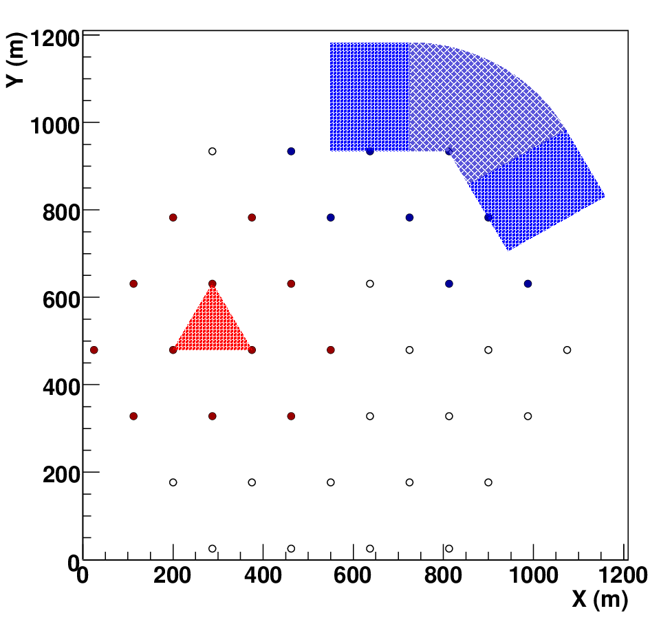
The Monte Carlo simulations are performed using the GrISU(tah) package [18]. We are interested in the performance of large arrays. Because of the relatively small field of view chosen, a telescope cannot effectively record images of showers with too large impact parameters. With , a 1 TeV-shower image is well contain in the camera only up to 300 m (Figure 4) and this worsens at higher energies. Most air showers will be detected only by a small fraction of the telescopes. Thus, we restrict our simulations to sub-arrays close to the shower-core impact point. The inside of a hexagonal array can be subdivided in triangular cells. In order to account for showers falling inside the array, we simulated showers inside a triangular cell and included the response of only the 12 closest telescopes around this cell. For the showers falling outside the array, we assume that the external shape of the array is a regular hexagon. The external belt can be subdivided in several regions of two types: the “sides” (next to telescopes aligned with their neighbors) and the “corners” (next to corner telescopes). Figure 9 shows the geometry of the different region types and the associated simulated sub-arrays. The results of these simulations can then be combined with different weights to characterize any size hexagonal arrays with more telescopes than in the simulated sub-array. A simple way to build a hexagonal array is to add hexagonal rings of telescopes around a central one. With rings we get telescopes, triangular cells, side regions and 6 corner regions. Here, we present results for arrays with from 19 to 469 telescopes.
With this approach, we are neglecting the fact that showers falling in triangular cells on the edge of the array are not surrounded by 12 telescopes but by only 9 or 8. However, the missing telescopes are distant from the shower and they are not expected to play a central role in the event detection and reconstruction. On the other hand, at high energy more telescopes than the 12 considered in the simulated sub-array will trigger. These additional images, even truncated, may slightly improve the angular resolution and CR rejection.
The Monte Carlo data are analyzed with one of the analysis chains used for the VERITAS data. Shower images recorded by each telescope are preprocessed with the standard two-threshold-cleaning algorithm. In order to be part of the image, a pixel must exceed a high threshold of 4 photo-electrons or exceed a low threshold of 2 photo-electrons and neighbor a pixel that exceeds the high threshold. With such small telescopes, the NSB per pixel and per integration gate is typically well below 1 photo-electron. A cleaned image is considered usable for event reconstruction when it is made of at least 4 pixels and contains at least 25 photo-electrons. An event is considered if 3 images satisfy the usability criteria. We use the same requirements for all pixel sizes. These requirements set the analysis-level energy threshold of the array.
The arrival direction of a good quality event is reconstructed by stereoscopy. For each pair of usable images a direction is reconstructed. The final reconstructed direction is obtained as the average of all the pairs directions with weights calculated as a function of the image sizes, image lengths and relative angle between the major axis of the two images. This multi-telescope stereoscopic analysis has been developed and validated for the 4-IACT array VERITAS.
4.3 Angular resolution
We first want to determine an optimal pixel size and continue our study with only one pixel size. In order to do this, we compared the angular resolution obtained for different camera pixelations. Figure 10 shows the -containment angle of the point spread function as a function of the -ray energy for 30∘ zenith angle showers falling inside the array for different pixel sizes. There is a clear improvement between and but almost no improvement from to . As a consequence, we choose for the rest of this study. Smaller pixels would results in rapidly increasing camera costs which are not justified by performance improvements. It should be noted that even are resulting in a very attractive angular resolution, better than 3′ above 10 TeV.

Figure 10 also shows the -containment radius for the array inside and outside regions with and compares them to the angular resolution of VERITAS [19]. The angular resolution of the inner region improves rapidely with the energy. Above 10 TeV, it is better than 2′. Our estimation is even conservative as only 12 telescopes are considered while more telescopes would in fact detect such high energy showers. The angular resolution becomes better than what is achieved with current telescope arrays above 2-3 TeV while our chosen pixel size is quite larger. This is due to the fact that in small arrays, a large fraction of events are showers falling outside where all the telescopes view the shower from a similar view point, making the stereoscopic reconstruction less effective. With a large array as well, the direction reconstruction of showers falling outside is clearly not as good as for showers falling inside. Selection of showers falling inside or close to the array would allow to achieve a very good angular resolution, but would reduce the effective area. An IACT array with very large inter-telescope distances, and correspondingly large field of views to reach for the highest energies, could not achieve a so good angular resolution. For example, the array with m, and the same pixel size studied in [20], would not achieve an angular resolution better than the current experiments even with a cut on the core impact distance.
4.4 Threshold and collection area
We simulated -ray showers with energies from 350 GeV to 100 TeV at 30∘ from zenith falling in a triangular cell and in the outside regions. Half the 1 TeV showers falling in a triangular cell are detected and pass our quality selection criteria. The energy threshold is around 1 TeV as we targeted when choosing the telescope diameter. For hexagonal arrays of various sizes, Figure 11 shows the effective collection area (at this level of event selection), as a function of energy. With a very large number of telescopes, is dominated by the inside array region which provides good angular resolution and result in a close to constant effective area above 1.6 TeV. With a small number of telescopes however, is dominated by the contribution from regions outside the array where the reconstruction performance is not as good. As higher energy showers can be detected further away in the outside region, depends on the energy. This effect is shower and telescope model dependent, thus opening up the possibility of systematic errors affecting the spectrum reconstruction.

As discussed earlier, 100 TeV astronomy requires at least 100 kmhr exposures. Generally IACT arrays are used to observe a given source not more than 50 hr per year. This sets a minimal requirement on the effective collection area to 2 km2 at 100 TeV which is achieved by the 61-telescope array. It should be noted that no more than 20 sources per year could be observed at the required exposure level for 100 TeV with the 61-telescope array while the present TeV sky already counts more than 70 sources. However, at lower energy, this array also offers a large collection area which would satisfy the exposure requirement of Figure 7 in a very short time. For example, in one hour, more than 25 events above 2 TeV from known sources would be collected. This would be enough for a detection if it were not for CR-background-discrimination issues.
4.5 Cosmic-ray discrimination and sensitivity
The sensitivity of a ground-based -ray observatory is its capability to detect a -ray source hidden in an isotropic background generated by the CR air showers, and to measure the flux of this source. IACT can reject most of CR events thanks to an image shape analysis and, in the case of sources which are not too extended, a selection of events from the small sky region of interest. The sensitivity depends on the observation time, the energy considered, the source characteristics (extension, spectrum) and the maximal flux-measurement uncertainty required. Here, we define the sensitivity as the minimum -ray flux above a given energy , for a 5-standard-deviation detection based on more than 10 events in 50 hr of observation of a point-like source with a power-law spectrum with an index .
In order to estimate the CR background, we need to determine the CR acceptance (collection area solid angle) and the CR-rejection efficiency. We simulated atmospheric Cherenkov signal for proton and -particle showers from 500 GeV to 500 TeV, with an energy distribution following a power law with spectral index of -2.7. We estimate with the same technique as for , subdividing the array into triangular cells and outside regions. We selected the -ray events by applying our standard analysis. In principle, the -ray-like-event-selection cuts should be carefully optimized. This would require a huge amount of CR-shower simulations not available for this study. Instead of a careful optimization, we have chosen our selection criteria by eye, comparing image-parameter distributions for rays and CR. The results presented here are therefore conservative. Using the CR flux measured with ATIC-2 [14], we estimate the background rate of CR events passing selection cuts with a reconstructed energy above the given energy and a reconstructed direction in the on-source region. The on-source region is defined as the 68%-containment radius for a -ray point source at energy .
Generally, observations are taken in wobble mode with the studied source
off-centered. The background level is then estimated from regions at the
same distance from the camera center (off-regions). Here, we assume
observation in wobble mode with an offset of 0.5∘ and a background
determined from 7 off-regions. Then, we calculate the number
of -ray events needed for a 5 standard-deviation
detection with the Li and Ma formula [21]. We also required
10. We finally obtain the sensitivity
as following:
where = 50 hr, and is the -ray-selection efficiency at the energy . Figure 12 shows for arrays of 61 telescopes and 469 telescopes in comparison with the sensitivity of VERITAS [19] and the Crab Nebula flux (considered here as a pure power-law spectrum with a spectral index of -2.5).

Current IACT observatories achieve their highest differential spectrum sensitivity, 1% Crab flux, between 300 GeV and 1 TeV. The 61-telescope example array could increase this energy range up to 10 TeV and improve the best sensitivity by a factor of two (0.5% Crab flux in the 1.5-5 TeV energy range). Above 1 TeV, the current IACT arrays get a good sensitivity because of a very efficient background rejection but they are rapidly limited by the -ray statistics. On the contrary, large IACT arrays obtain large statistics and their background rejection improves rapidly with the energy. Sensitivity of our 61-telescope array is already 10 times better than VERITAS above 5 TeV and 25 times above 10 TeV. This sensitivity estimate is even very conservative because here the background discrimination has not been optimized. At higher energy, the sensitivity is much better than any existing experiment and one could measure the spectrum of a ()%-Crab-flux source above 100 TeV in 50 hr. A dozen of known galactic sources should be measured up to 100 TeV. Many unknown sources with hard spectra may also be detected. For instance, a 1%-Crab-flux source above 250 GeV with spectral index of -2 has a 20%-Crab flux above 100 TeV.
With 469 telescopes, the sensitivity curve has essentially the same shape as with 61 telescopes but with a factor of 3 improvement. This means that with the 469-telescope array, one can reach about the same sensitivity as with the 61-telescope array in one tenth of the time (except the highest energies where the sensitivity is driven by the number of -ray events rather than by the CR-background rejection). Then, one could study hundreds of sources per year in the 1-10 TeV energy range. Above 100 TeV, the sensitivity is 8%-Crab flux and, even if our study for rays stops at 100 TeV, it is clear that such large arrays would have useful sensitivities up to a few hundreds of TeV.
With larger telescopes or higher quantum efficiency cameras, the sensitivity curve can be expected to essentially shift to the left. Energy threshold would be lower and the sensitivity would strongly improve below 10 TeV. At the highest energy the array performances would remain more or less the same.
5 Conclusion
The next generation of IACT arrays is currently in design phase. We investigated the performance of large uniform arrays of IACTs. For the optimization, we chose to maximize the effective collection area for a given energy threshold and price. From considerations on the atmospheric Cherenkov light properties and pricing, we found that the optimal uniform IACT array is a hexagonal-lattice array with a 175 m inter-telescope spacing. The diameter of the telescopes depends on the targeted energy threshold while the camera field of view depends on the maximal energy to be covered. Additionally, provisions for the effective -ray field of view must also be made. The 1 TeV -ray astronomy is particularly interesting as it could allow the identification of cosmic-ray accelerators up to the knee energy. Following the optimal design prescriptions obtained, we designed a -ray observatory dedicated to the 1 TeV-100 TeV energy range. We conservatively based our simulation on existing telescopes, electronics and data analysis. We showed that an array of 61 telescopes of 3 m diameter equipped of 5∘ field of view camera with 499 pixels would improve the sensitivity above a few TeV by an order of magnitude, and could measure spectrum up to 100 TeV for 25%-Crab-flux sources (a dozen of known galactic sources could reach this flux above 100 TeV). The large effective area achieved above a few TeV allows to reduce the observation time without being limited by the -ray statistic contrary to the current experiments at these high energies. This is important as the observation time per source will decrease as the number of sources increases. The very good angular resolution achieved at high energy ( 2′) plays an important role for the morphology study and source disambiguation as galactic sources are typically extended and concentrated in the galactic plane.
6 Acknowledgment
The authors are grateful to Pierre Sokolsky for his support and to Masahiro Teshima and the StarBase Utah team for informations about the 7 T.A. telescopes.
References
- (1) Aharonian, F., Buckley, J., Kifune, T. and Sinnis, G., 2008, IOP PUBLISHING, Rep. Prog. Phys. 71 (2008) 096901 (56pp)
- (2) Wakely, S. and Horan, D., (2008) http://tevcat.uchicago.edu/
- (3) Kertzman, M.P. and G.H. Sembroski, Nucl. Instr. Meth. Phys. Res. A 343 (1994), 629
- (4) Aharonian, F. et al., A&A 464 (2007), 235
- (5) Aharonian, F. et al., A&A 437 (2005), L7
- (6) Atwood, W.B. et al., arXav:0902.1089, submitted to ApJ (2009)
- (7) Moskalenko, I. V. et al., ApJ 640 (2006), L155
- (8) Aharonian, F. et al., ApJ 636 (2006), 777
- (9) Colin, P., LeBohec, S. and Holder, J., J. of physics: conference series 60 (2007), 303
- (10) Aharonian, F. et al., ApJ 614 (2004), 897
- (11) Aharonian, F. et al.,A&A 425 (2004) L13
- (12) Aharonian, F. et al., A&A 435 (2005), L17
- (13) Acciari, V. A. et al., ApJ 679 (2008), 1427
- (14) Panov, A.D. et al., Bull. Russ. Acad. Sci. Phys. 71 (2007), 494
- (15) Yamamoto et al., Astropart. Phys. 11 (1999), 141
- (16) http://www.physics.utah.edu/starbase/
- (17) LeBohec, S. and Holder, J., Astropart.Phys. 19 (2003) 221-233
- (18) http://www.physics.utah.edu/gammaray/GrISU/
- (19) Holder, J. et al., AIP Conf. Proc., 1085 (2008), 657
- (20) Funk, S. and J.A. Hinton, AIP Conf. Proc., 1085 (2008), 882
- (21) Li, T. P. & Ma, Y. Q. ApJ 272 (1983), 317